A CHARACTERIZATION OF THE BANZHAF - isical.ac.inrana/sensitivity.pdf · A CHARACTERIZATION AND SOME...
27
1 A CHARACTERIZATION AND SOME PROPERTIES OF THE BANZHAF-COLEMAN-DUBEY-SHAPLEY SENSITIVITY INDEX 1 Rana Barua, Statistics-Mathematics Unit, Satya R. Chakravarty, Economic Research Unit, Sonali Roy, Economic Research Unit, Palash Sarkar, Applied Statistics Unit, Indian Statistical Institute, Kolkata, India. Correspondent: Satya R. Chakravarty Economic Research Unit Indian Statistical Institute 203 B.T. Road Kolkata – 700108 INDIA Fax: 913325778893 e-mail: [email protected] 1 For comments and suggestions, we are grateful to two anonymous referees.
Transcript of A CHARACTERIZATION OF THE BANZHAF - isical.ac.inrana/sensitivity.pdf · A CHARACTERIZATION AND SOME...
1
A CHARACTERIZATION AND SOME PROPERTIES OF THE
BANZHAF-COLEMAN-DUBEY-SHAPLEY SENSITIVITY INDEX1
Rana Barua, Statistics-Mathematics Unit,
Satya R. Chakravarty, Economic Research Unit,
Sonali Roy, Economic Research Unit,
Palash Sarkar, Applied Statistics Unit,
Indian Statistical Institute, Kolkata, India.
Correspondent:
Satya R. Chakravarty
Economic Research Unit
Indian Statistical Institute
203 B.T. Road
Kolkata – 700108
INDIA
Fax: 913325778893
e-mail: [email protected]
1For comments and suggestions, we are grateful to two anonymous referees.

2
Abstract
A sensitivity index quantifies the degree of smoothness with which it responds to
fluctuations in the wishes of the members of a voting body. This paper characterizes the
Banzhaf (1965)-Coleman (1971)- Dubey-Shapley (1979) sensitivity index using a set of
independent axioms. Bounds on the index for a very general class of games are also
derived.
JEL Classification Numbers: C71, D72.
AMS 2000 Classification: Primary- 91A06; Secondary- 91A40.
Key words: voting game, the Banzhaf – Coleman – Dubey- Shapley sensitivity index,
characterization, bounds.

3
1. Introduction
A sensitivity index is a measure of the extent of volatility in a decision rule
(voting body). It is an indicator of the degree of ease with which it responds to the
fluctuations in the wishes of the members of the voting body. It can as well be regarded
as a democratic participation index measuring sensitivity to the desires of the voting body
members.
Dubey and Shapley (1979) considered the sum of the numbers of swings of
different voters in a voting game as a sensitivity index, where the number of swings of a
voter is the number of winning coalitions from which the defection of the voter makes
them losing. (A coalition is called winning if the sum of the ‘yea’ votes of the members
of the coalition can guarantee the passage of a resolution. A coalition is called ‘losing’ if
it is not winning). Thus, this index gives the numbers of possibilities in which different
voters are in the critical position of being able to change the voting outcome by changing
their votes. Since a critical voter’s exit from a winning coalition makes it losing, it gives
an indication that even a single voter could tip the scales. A normalized version of the
Dubey-Shapley index was considered by Felsenthal and Machover (1998) for measuring
sensitivity. We refer to this normalized formula, which is the sum of one of the
Banzhaf(1965)-Coleman(1971) indices of power of different voters in the game, as the
Banzhaf-Coleman-Dubey-Shapley (BCDS) sensitivity index.
Dubey and Shapley (1979) investigated several properties of their index,
including determination of lower and upper bounds. A feasible and desirable direction of
research along this line is to study additional/alternative properties of the BCDS index
and characterize it uniquely. This is the objective of this paper. More precisely, we first
discuss some properties and develop an axiomatic characterization of the BCDS
sensitivity index. It is shown that the set of axioms used in the characterization theorem is
minimal, that is, no proper subset of this set can characterize the index. Equivalently, we
say that axioms belonging to this minimal set are independent. Then using Fourier
Transform analysis, we derive some additional properties and bounds for the BCDS
index for a c1965
88 Tw(s )Tj8.27998 sTd(()Tj3.959990.036 Tc1.836 Tw(r )Tj98.52 0 Td(d)Tjatem.

4
The next section of the paper sets out the background material. Section 3 defines
the BCDS index and discusses some of its properties. Section 4 derives the index
axiomatically and demonstrates independence of the properties employed in the
axiomatization exercise. In Section 5 we discuss some additional properties of the index,
including derivation of bounds, using Fourier Transform. Finally, Section 6 concludes the
paper.
2. The Background
It is possible to model a voting situation as a coalitional form game, the hallmark
of which is that any subgroup of players can make contractual agreements among its
members independently of the remaining players. Let { }nN ,...,2,1= be a set of players.
The power set of N, that is, the collection of all subsets of N , is denoted by N2 . Any
member of N2 is called a coalition. A coalitional form game with player set N is a pair
( )VN; , where RV N →2: such that ( ) 0=φV , where R is the real line. For any
coalition S , the real number ( )SV is the worth of the coalition, that is, this is the amount
that S can guarantee to its members. For any set S, S will denote the number of
elements in S.
We frame a voting system as a coalitional form game by assigning the value 1 to
any coalition which can pass a bill and 0 to any coalition which cannot. In this context, a
player is a voter and the set { }nN ,...,2,1= is called the set of voters. Throughout the
paper we assume that voters are not allowed to abstain from voting. A coalition S will be
called winning or losing according as it can or cannot pass a resolution.
Definition1: Given a set of voters N , a voting game associated with N is a pair ( )VN; ,
where { }1,02: →NV satisfies the following conditions:
(i) ( ) 0=φV .
(ii) ( ) .1=NV
(iii) If ,TS ⊆ ,2, NTS ∈ then ( ) ( ).TVSV ≤

5
The above definition formalizes the idea of a decision-making committee in
which decisions are made by vote. It follows that the empty coalition φ is losing
(condition (i)) and the grand coalition N is winning (condition (ii)). All other coalitions
are either winning or losing. Condition (iii) can be regarded as a monotonicity principle.
It ensures that if a coalition S can pass a bill, then any superset T of S can pass it as
well. A game ( )VNG ;= is called proper if for NTS 2, ∈ , ( ) ( ) 1== TVSV implies that
φ≠∩TS . According to this condition, two winning coalitions cannot be disjoint. The
collection of all voting games is denoted by F. For any ( )VNG ;= , we write ( )GG LW
for the set of all winning (losing) coalitions associated with G. Thus, for any NS ⊆ ,
( ) )0(1=SV is equivalent to the condition that ∈S ( )GG LW .
Definition 2: A voting game ( )VNG ;= is called
(i) decisive if for all ,2 NS ∈ ( ) ( ) 1=−+ SNVSV ,
(ii) balanced if 12 −== NGG LW .
Clearly, a decisive game is balanced.
Definition 3: The unanimity game ( )NUN; associated with a given set of voters N is the
game whose only winning coalition is the grand coalition N.
Definition 4: Given a set of voters N , let ( )VN; be a voting game.
(i) For any coalition ,2 NS ∈ we say that Ni ∈ is swing in S if ( ) 1=SV but
{}( ) 0=− iSV .
(ii) A coalition NS 2∈ is said to be minimal winning if ( ) 1=SV but there does not
exist ST ⊂ such that ( ) 1=TV .
Thus, voter i is swing, also called pivotal or key, in the winning coalition S if his
deletion from S makes the resulting coalition {}iS − losing. For any game
( ) F∈= VNG ; , and Ni ∈ , we write ( )Gmi to denote the number of winning coalitions

6
in which voter i is swing. It is often said that ( )Gmi is the number of swings of voter i .
We will indicate the total number of swings ( )∑=
N
ii Gm
1
in G by ( )Gm .
Definition 5: For a set of voters N , let ( )VN; be a voting game. A voter Ni ∈ is called
a dummy in ( )VN; if he is never swing in the game. A voter Ni ∈ is called a
nondummy in ( )VN; if he is not dummy in ( )VN; .
Following Felsenthal and Machover (1998) we have
Definition 6: For a voting game ( )VN; with the set of voters ,N a voter Ni ∈ is called a
dictator if {}i is the sole minimal winning coalition in the game.
By definition, a dictator in a game is unique. If a game has a dictator, then he is the only
swing voter in the game.
A very important voting game is a weighted majority game.
Definition 7: For a set of voters { }nN ,...,2,1= , a weighted majority game is a quadruplet
( )qVNG ;;; w= , where ( )nwww ,..., 21=w is the vector of nonnegative weights of the
N voters in N, q is a positive real number quota such that ∑≤=
N
iiwq
1 and for any NS 2∈ ,
( ) 1=SV if qwSi
i ≥∑∈
= 0 otherwise.
That is, the thi voter casts iw votes and q is the quota of votes needed to pass a bill. A
weighted majority game will be proper if qw
N
ii
<∑
=2
1 . Note that a weighted majority
game satisfies conditions (i)-(iii) of definition 1. (See Felsenthal and Machover, 1998, for
further discussions on definitions 1 and 7.)

7
3. The Banzhaf-Coleman-Dubey-Shapley Sensitivity Index
For any ( )G N V= ∈; F , we call mi ( )G the first Banzhaf-Coleman index of
voting power of i N∈ . The second and third Banzhaf-Coleman indices of voting power
are given respectively by ( )
12 −Ni Gm
and ( )( )GmGmi .
Earlier, Shapley and Shubik(1954) suggested an index of voting power defined as
the number of orderings in which the concerned voter is swing divided by the total
number of orderings of the voters. (See Dubey and Shapley, 1979; Felsenthal and
Machover, 1995 and Burgin and Shapley, 2001, for further discussion.) Alternatives and
variations of these indices were suggested, among others, by Deegan and Packel (1978),
Johnston (1978) and Barua et al. (2002).
Dubey and Shapley (1979) suggested the use of
( ) =GD ( )Gm (1)
as a sensitivity index, where F∈G is arbitrary. The Felsenthal –Machover (1998)
version of this index is given by
( ) ( )12 −
=N
GmGB . (2)
Since ( )GB is the sum of the second Banzhaf-Coleman indices of different voters in a
game, we refer to ( )GB as the Banzhaf-Coleman-Dubey-Shapley (BCDS) index of
sensitivity. It ‘reflects the ‘‘volatility’’ or degree of suspense in the voting body’ (Dubey
and Shapley, 1979). Suppose in a voting game each voter’s probability of voting for or
against a bill is selected independently from a uniform distribution [0,1]. Then
12 −Nim becomes the probability ip that other voters will vote such that the bill will
pass or fail according as i votes for or against it (Straffin, 1977). The index )(GBi is
simply ∑=
N
iip
1.
The index B possesses the following interesting properties.

8
(a) Anonymity: Let ( )VNG ;= and ( ) F∈′′=′ VNG ; be two isomorphic games. That is,
there exists a bijection h on N onto N ′ such that for all NS ⊆ , ( ) 1=SV if and only if
( )( ) 1=′ ShV , where ( ) ( ){ }SxxhSh ∈= : . Then ( ) ( )GBGB ′= .
(b) Increasingness: Let ( )VNG ;= and ( )VNG ;= F∈ be two games such that N = N
and ( ) ( )GmGm ii ≥ for all Ni ∈ with > for at least one Ni ∈ . Then ( ) ( )GBGB > .
( c) Dummy Independence Principle: For any ( )VNG ;= F∈ and for any dummy
Nd ∈ , ( ) ( )dGBGB −= , where dG− is the game obtained from G by excluding d .
Likewise, ( ) ( )dGBGB += , where dG+ is the game obtained from G F∈ by including
d as a dummy.
(d) Maximality: For any ( )VNG ;= F∈ , ( )GB attains its maximal value 12 −
N
r
Nr
if and
only if all coalitions with more than 2
N voters win and all coalitions with less than
2
N
voters lose, where 12
+
=
Nr , with [ ]x being the largest integer x≤ (Dubey and
Shapley, 1979).
(e) Duality: For any ( )VNG ;= F∈ , let ( )∗∗ = VNG ; be the dual of G , that is ( )SV ∗ =
( ) ( )SNVNV −− for all NS 2∈ . Then ( ) ( )∗= GBGB (Dubey and Shapley, 1979).
Anonymity says that a reordering of the voters does not change the sensitivity
index B . Thus, all characteristics other than swings of the voters, e.g., their living
conditions, are irrelevant to the measurement of sensitivity. Increasingness requires the
index B to be an increasing function of the number of swings, given that the voter set
remains unaltered. To understand increasingness, let us consider the weighted majority
game ( )4;2,2,1;;ˆ0 VNG = obtained from ( )3;2,2,1;;0 VNG = by augmenting the quota
from 3 to 4. Given that the set of voters { }3,2,1=N is the same in the two games, we get
( ) ( )0202 GmGm = =2, ( ) ( )0303 GmGm = =2 and ( ) ( ) 0ˆ2 0101 =>= GmGm . We thus have
( ) ( )00 GBGB > . Since a dummy is not able to influence the voting outcome, we can argue

9
that B should satisfy the dummy independence principle. Given that the second Banzhaf-
Coleman voting power index ( )
12 −Ni Gm
remains invariant under inclusion or exclusion of a
dummy (Owen (1978), Felsenthal and Machover, 1995, 1998 and Barua et al., 2002), B
also satisfies this invariance condition. Maximality specifies the necessary and sufficient
condition for B to achieve the maximum value and duality shows that the values of B
for a voting game and its dual are the same.
Dubey and Shapley (1979) showed that for any ( ) F∈= VNG ; ,
( ) [ ]1
2
2
log−
−≥
N
NGB
θθ (3)
where θ is the minimum of the numbers of winning and losing coalitions in G . Hart
(1976) suggested a stronger but more complicated lower bound for ( )GB . Dubey and
Shapley (1979) also noted that if G is a decisive game, then a lower bound of ( )GB is
1.
Examples of sensitivity indices other than ( )GB which satisfy properties (a) –(e)
are ( )( )cGB , 1,0 ≠> cc and ( )( )GBexp . However, because of its probabilistic
interpretation, expositional and computational ease, ( )GB appears to be more attractive
than such indices. Furthermore, in the next section we show that a characterization of
( )GB can be developed using a set of intuitively reasonable axioms. These therefore
make ( )GB a desirable index of sensitivity.
4. The Characterization Result
In order to present the axioms that characterize the BCDS index, we need the
following definitions.
Definition 8: Given ( ) ( ) F∈== 222111 ;,; VNGVNG , where 1N and 2N need not be
disjoint, we define 21 GG ∨ as the game with the set of voters 21 NN ∪ , where a coalition
⊆S 21 NN ∪ is winning if and only if ( ) 111 =∩ NSV or ( ) 122 =∩ NSV .

10
Definition 9: Given ( ) ( ) F∈== 222111 ;,; VNGVNG , we define 21 GG ∧ as the game
with the set of voters 21 NN ∪ , where a coalition ⊆S 21 NN ∪ is winning if and only if
( ) 111 =∩ NSV and ( ) 122 =∩ NSV .
Thus, in order to win in 21 GG ∨ a coalition must win in either 1G or 2G , whereas to win
in 21 GG ∧ it has to win in both 1G and 2G . Clearly, given F∈21 ,GG ;
21 GG ∨ , 21 GG ∧ F∈ .
Finally, we have
Definition 10: Given ( ) F∈VN; , suppose that the voters Nji ∈, are amalgamated into
one voter ij . Then the post-merger voting game is the pair ( ) F∈′′ VN ; , where
{ } { }ijjiNN ∪−=′ , and
( ) ( )SVSV =′ if { }ijNS −′⊆ ,
{ }( ) { }( )jiijSV ,∪−= if Sij ∈ .
We are now in a position to present three axioms on a general sensitivity index
RP →F: that will uniquely isolate the BCDS index. The first axiom is taken from
Dubey (1975) (see also Dubey and Shapley, 1979). It shows how the sensitivity levels in
the games G G1 2∨ and G G1 2∧ are related to individual sensitivities in G1 and G2 .
Axiom A1 (Sum Principle): For any G1 , G2 ∈F ,
( ) ( ) ( ) ( )212121 GPGPGGPGGP +=∧+∨ . (4)
This axiom, which is also referred to as linearity / union-intersection property in the
literature, is quite similar to the condition characterizing additive measures (in measure
theoretic sense), such as probabilities. If 1A and 2A are two events in a probability space
and ∨ and ∧ are the disjunction and conjunction operations respectively, then
( ) ( ) ( ) ( )212121 APAPAAPAAP +=∧+∨ , where P denotes probability.
The next axiom captures the change in sensitivity levels under a merger of any
two voters in an unanimity game. In an unanimity game the number of swings of each
voter is only one. Now, in a voting game the power of a voter is determined by his swings
only. Since the number of swings across voters in unanimity games is a constant (=1), an
important source of difference between the extents of sensitivity in two such games is the
number of voters. One way of reflecting this difference is to assume that the ratio

11
between sensitivity levels in an unanimity game and a new game obtained by merging
two voters in this game is proportional to the ratio of the numbers of voters in them. The
following axiom gives a formulation along this direction.
Axiom A2 (Proportionality Principle): Let F∈′G be the game obtained from
( ) F∈= NUNG ; by merging two voters i j N, ∈ . Then,
( )( ) N
N
GPGP
′=
′ 21
. (5)
The third axiom is a normalization condition that states the value of the index if
the game has a dictator.
Axiom A3 (Normalization): If ( )G N V= ∈; F has a dictator, then ( ) 1=GP .
Since the BCDS index is obtained directly from the second Banzhaf-Coleman
index, a comparison of our axioms with some existing axiom systems that characterize
the latter will be worthwhile. Lehrer (1988) characterized the second Banzhaf-Coleman
index using the sum criterion A1 and a two-voter superadditivity property, which is
similar to, but weaker than A2, along with Shapley’s (1953) dummy axiom and an equal
treatment principle. An alternative characterization of this index was developed by
Nowak (1997) using a version of Lehrer’s (1988) superadditivity property, equal
treatment principle, dummy axiom and a postulate of Young (1985) which says that the
power is (in some sense) determined by the marginal contributions of voters. An
important difference of Nowak’s axiomatization with Lehrer’s exercise (and also ours) is
that the former does not make use of the additivity axiom A1.
We now have
Theorem 1: A sensitivity index P satisfies axioms A1-A3 if and only if it is the
Banzhaf-Coleman-Dubey-Shapley sensitivity index B given by (2).
Proof: We first demonstrate that B satisfies A1-A3. Let ( )G N V1 1 1= ; , ( )G N V2 2 2= ;
∈F . Assuming that φ≠− 21 NN , take i N N∈ −1 2 . Now, any coalition 12 NNS −⊆′
can be appended to a swing coalition S N⊆ 1 for i N∈ 1 to obtain a swing coalition
S S∪ ′ for i N N∈ ∪1 2 unless ( )S S N∪ ′ ∩ 2 is winning in G2 . Hence the number of
swings of voter 21 NNi −∈ is
( ) ( ) ( )m G G m G m G Gi iN N
i1 2 1 1 22 2 1∨ = − ∧−
12
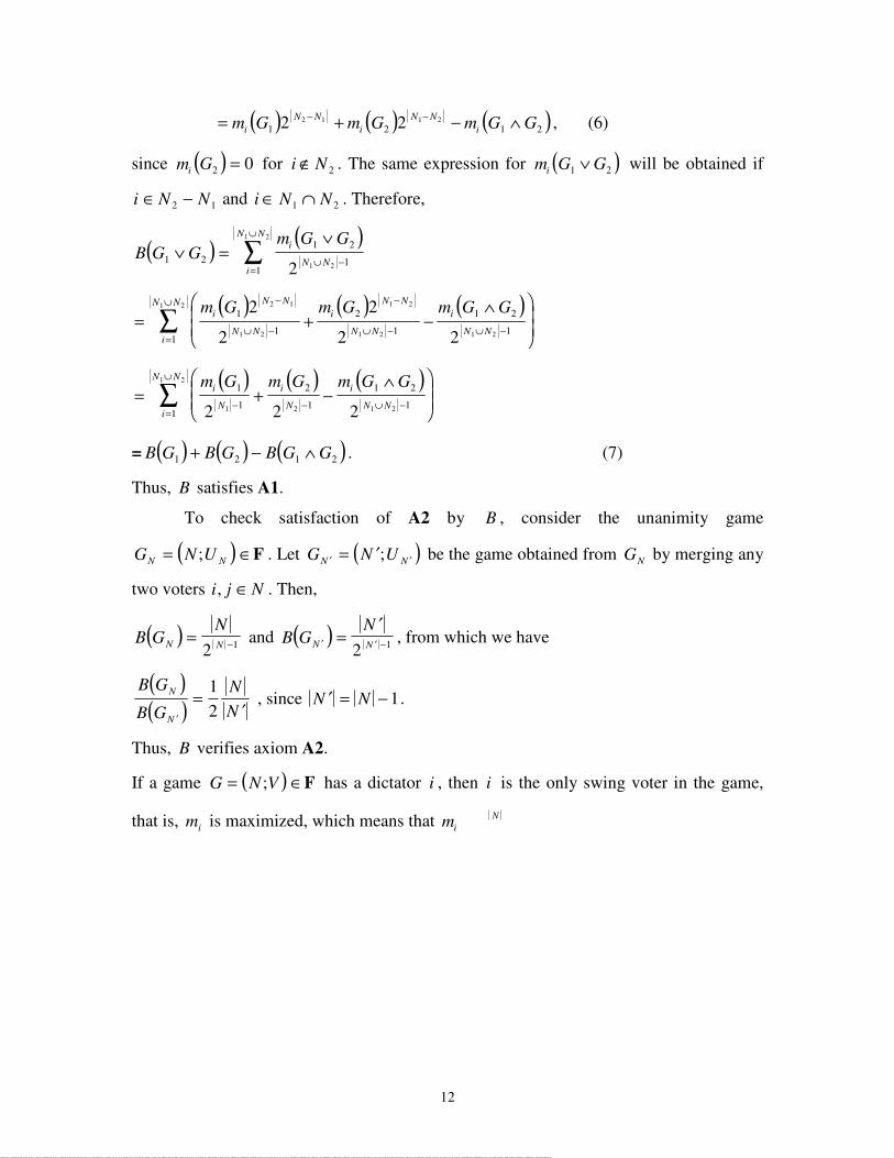
( ) ( ) ( )= + − ∧− −m G m G m G GiN N
iN N
i1 2 1 22 22 1 1 2 , (6)
since ( )m Gi 2 0= for 2Ni ∉ . The same expression for ( )m G Gi 1 2∨ will be obtained if
i N N∈ −2 1 and ∈i N N1 2∩ . Therefore,
( ) ( )B G G
m G Gi
N Ni
N N
1 21 2
11 2 1 2
1 2
∨ =∨
∪ −=
∪
∑
( ) ( ) ( )= + −
∧
−
∪ −
−
∪ − ∪ −=
∪
∑ m G m G m G GiN N
N N
iN N
N N
i
N Ni
N N1
1
2
1
1 2
11
2
2
2
2 2
2 1
1 2
1 2
1 2 1 2
1 2
( ) ( ) ( )= + −
∧
− − ∪ −
=
∪
∑ m G m G m G Gi
N
i
N
i
N Ni
N N1
1
2
1
1 2
11 2 2 21 2 1 2
1 2
= ( ) ( ) ( )B G B G B G G1 2 1 2+ − ∧ . (7)
Thus, B satisfies A1.
To check satisfaction of A2 by B , consider the unanimity game
( )G N UN N= ∈; F . Let ( )G N UN N′ ′= ′; be the game obtained from NG by merging any
two voters i j N, ∈ . Then,
( )B GN
N N= −2 1 and ( )B GN
N N′ ′ −=′
2 1 , from which we have
( )( )
B G
B GNN
N
N ′
=′
12
, since ′ = −N N 1.
Thus, B verifies axiom A2.
If a game ( )G N V= ∈; F has a dictator i , then i is the only swing voter in the game,
that is, im is maximized, which means that miNN2
m

13
kSSS ,..., 21 are minimal winning coalitions of G and iSG is the unanimity game
corresponding to iS , ki ,...,2,1= . Thus, by A1, P is determined if ( )1SGP ,
( )

14
unanimity game corresponding to iS , 2,1=i and ( )NN UNG ;~ = . Then ( )=GB
~ +−122
2
25.12
32
21312 =− −− .
We will now show that axioms A1-A3 are independent. Demonstration of
independence requires that if one of these three axioms is dropped, then there will exist a
sensitivity index that will satisfy the two remaining axioms but not the dropped one.
Theorem 2: Axioms A1-A3 are independent.
Proof: Let ( )VNG ;= F∈ be arbitrary. Then consider the sensitivity indices given by
( )N
N
iim
GP21
1
∑== , (9)
( )21
21
2 +=∑
=N
N
iim
GP (10)
( ) ( )1
log1
2
3 −
=∑
=
N
m
GP
N
ii
, 2>N . (11)
It is easy to see that 1P verifies A1 and A2 but not A3, whereas 2P verifies A1 and A3
but not A2. One can also check that 3P fulfils A2 and A3 but not A1. �
5. Fourier Transform Analysis of the Banzhaf - Coleman -Dubey - Shapley
Sensitivity Index
In this section we analyze voting games using tools from Boolean function
literature. Before embarking on the details of the analysis, we discuss the connection of
games to Boolean functions and the main results that we obtain.
An n -variable Boolean function is a map { } { }1,01,0: →nf , where { }n1,0 is the
n -fold Cartesian product of { }1,0 . With the conventional identification of n - bit strings
15
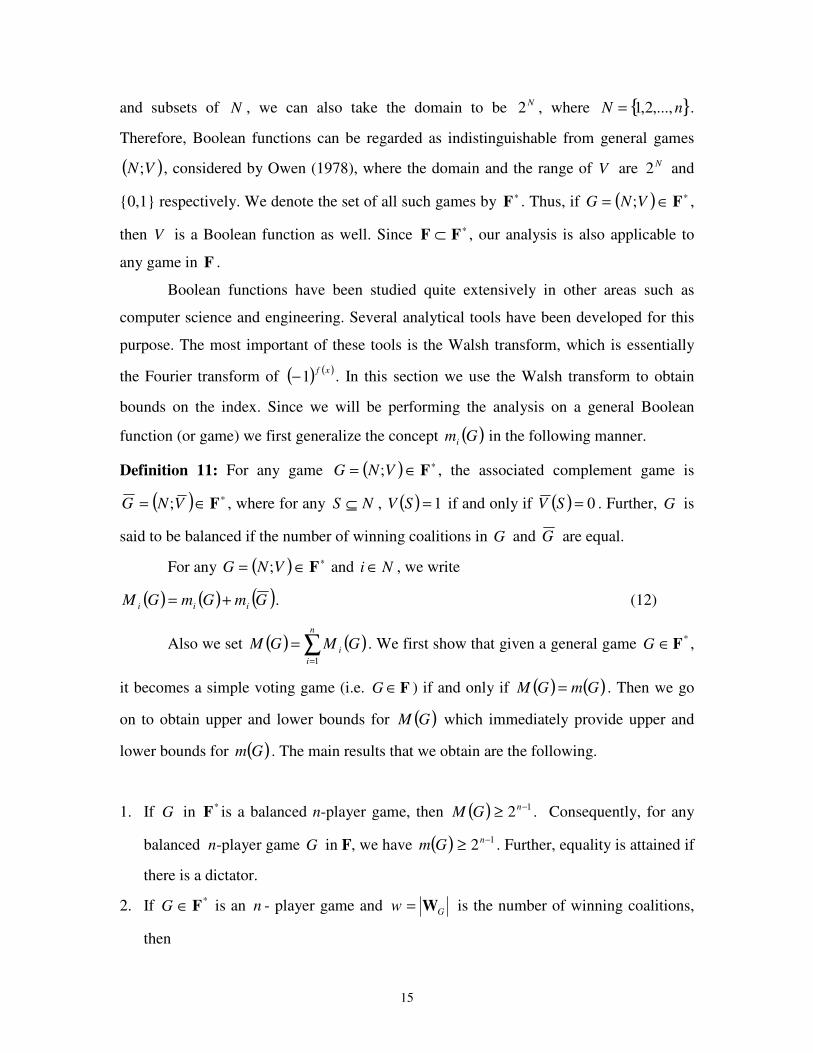
and subsets of N , we can also take the domain to be N2 , where { }nN ,...,2,1= .
Therefore, Boolean functions can be regarded as indistinguishable from general games
( )VN; , considered by Owen (1978), where the domain and the range of V are N2 and
{0,1} respectively. We denote the set of all such games by ∗F . Thus, if ( )VNG ;= ∈ ∗F ,
then V is a Boolean function as well. Since ⊂F ∗F , our analysis is also applicable to
any game in F .
Boolean functions have been studied quite extensively in other areas such as
computer science and engineering. Several analytical tools have been developed for this
purpose. The most important of these tools is the Walsh transform, which is essentially
the Fourier transform of ( ) ( )xf1− . In this section we use the Walsh transform to obtain
bounds on the index. Since we will be performing the analysis on a general Boolean
function (or game) we first generalize the concept ( )Gmi in the following manner.
Definition 11: For any game ( )VNG ;= ∈ ∗F , the associated complement game is
( )VNG ;= ∈ ∗F , where for any NS ⊆ , ( ) 1=SV if and only if ( ) 0=SV . Further, G is
said to be balanced if the number of winning coalitions in G and G are equal.
For any ( )VNG ;= ∈ ∗F and Ni ∈ , we write
( ) ( ) ( )GmGmGM iii += . (12)
Also we set ( ) ( )∑=
=n
ii GMGM
1
. We first show that given a general game G *F∈ ,
it becomes a simple voting game (i.e. F∈G ) if and only if ( ) ( )GmGM = . Then we go
on to obtain upper and lower bounds for ( )GM which immediately provide upper and
lower bounds for ( )Gm . The main results that we obtain are the following.
1. If G in *F is a balanced n-player game, then ( )GM ≥ 12 −n . Consequently, for any
balanced n-player game G in F, we have ( )Gm ≥ 12 −n . Further, equality is attained if
there is a dictator.
2. If G ∈ *F is an n - player game and w GW= is the number of winning coalitions,
then

16
( )12
2−
−n
n ww ≤ ( )GM ≤ n( )
122
−
−n
n ww.
Further, both the upper and lower bounds are attained.
Consequently, for any n-player game G ∈ F we have ( ) ( ) nGm
wwn
n
≤≤−−12
2 ( )12
2−
−n
n ww.
Remarks:
(a) From result (1) above, it follows that for a decisive voting game, a lower bound of
( )GB is 1. As stated earlier, Dubey and Shapley (1979) derived 1 as the lower bound
of B for decisive voting games. Evidently, Corollary 16 presents a lower bound for a
more general class of games viz., balanced voting games. Moreover, Dubey and
Shapley’s (1979, p.108) claim that the lower bound can only be derived by using
Hart’s (1976) bound does not appear to be true.
(b) It is known (Felsenthal and Machover, 1998, p.56) that for F∈G , ( ) nGm ≥ . Result
(2) above provides a lower bound on ( )Gm for monotone games. This lower bound
depends on the number of winning coalitions. Though this can be lower than n , in
general it is going to be a sharper lower bound. In fact, our lower bound ( )
122
−
−n
n ww is
greater than n if 22
122 111 nn
wn
nn ≅−−> −−− .
To obtain these results, we first prove a relation (Lemma 9) between ( )GM i and
the autocorrelation function of the Boolean function associated with G . (See equation
(17) below for the definition of the autocorrelation function.) Thus, autocorrelation
function becomes a helpful technique in studying swings in general voting games.
Further algebraic analysis is performed using the Walsh transform which ultimately leads
to the desired results. This in turn establishes the role of the Walsh transform in proving
results in general voting games. Since the Walsh transform can be expressed in matrix
form using the Hadamard matrix, this motivates the use of the Hadamard matrix.
For the sake of convenience, we divide this section into two subsections.

17
5.1 Basics of Fourier Transform Analysis
In this subsection, we present the mathematical preliminaries necessary for
understanding the Fourier transform analysis of games.
Let 2F be the field { } ⋅⊕,,1,0 , where ⊕ and . denote modulo 2 addition and
multiplication. We thus consider the domain of a Boolean function to be the vector space
⊕,2nF over 2F , where, as stated, ⊕ is the addition operator on 2F and also on nF2 .
The inner product of two vectors ( )nuuu ,...1= , ( )nvvv ,...,1= ∈ nF2 is i
n
iivu∑
=1
and will be
denoted by vu, . The weight of an n -bit vector u is the number of ones in u and will
be denoted by ( )uwt .
The Fourier Transform is the most widely used tool in the analysis of Boolean
functions. In most cases it is convenient to apply Fourier Transform to ( ) ( )xf1− instead of
( )xf . The resulting transform is called the Walsh Transform of ( )xf . More precisely,
the Walsh Transform of ( )xf is an integer-valued function { } [ ]nnnfW 2,21,0: −→
defined by (see, for example, Ding et. al., 1991)
( ) ( ) ( )∑∈
⊕−=nFw
wuwff uW
2
,1 . (13)
The Walsh Transform is called the spectrum of f . Note that the spectrum measures the
cross-correlations between a function and the set of linear functions. Another way of
looking at the spectrum is via Hadamard matrices. Let nH be the Hadamard matrix of
order n2 defined recursively as (see MacWilliams and Sloane, 1977)
−
=11
111H (14)
11 −⊗= nn HHH for 1>n ,
where ⊗ denotes the Kronecker product of two matrices. For example,
−
=11
112 HH
HHH =
−−−
−
−−
1111
1111
1111
1111
.

18
Considering the rows and columns of nH to be indexed by the elements of nF2 , we
obtain [ ]( ) ( ) vuvunH ,
, 1−= . Using this fact, the Walsh Transform can be written as
( ) ( ) ( ) ( )[ ] ( ) ( )[ ]12,...,01,...,1 120 −=−− − nffn
ff WWHn
, (15)
where ∈u nF2 is identified with an integer in [
∈
rinsforn

19
Applying the inverse transform gives ( ) ( ) nf
n
Fuf CuW
n
22 2022
==∑∈
. This is a conservation
law for the spectral values of f and is known as Parseval’s Theorem (see, for example,
Ding et al., 1991).
The next result states a useful property of Walsh Transform (see Canteaut et.al.,2000,
Proposition 5). For a vector space E , we define ⊥E to be the vector space which is
orthogonal to E , i.e., ⊥E = { }Evvuu ∈∀= ,0,: .
Theorem 4: Let f and g be n -variable functions and E be a subspace of nF2 . Then
( ) ( )∑∑⊥∈∈
=Eu
fEw
f uCEwW 2 (19)
See (Sarkar and Maitra, 2002) for a discussion of the above results in a more general
setting.
5.2 The Results
In this subsection, we present the results mentioned at the beginning of section 5
along with complete proofs. First we generalize the notion of swing. The notion of swing
is quite general in the sense that we do not require monotonicity (condition (iii) in
definition1) for swing to be defined.
Definition 12: Given a game ( )VNG ;= ∈ ∗F , and Ni ∈ , number of negative swings of
i is defined as
( ) {} ( ) {}( ){ }1: =∪−−⊆=− iSVSViNSGmi .
For any ( )VNG ;= ∈ ∗F , we write
( ) ( )∑∈
−− =Ni
i GmGm . (20)
The following proposition, whose proof is very easy, states the relationship between
( )Gmi− and ( )Gmi .
Proposition 5: Let ( )VNG ;= ∈ ∗F be arbitrary. Then for any Ni ∈ , ( )Gmi− = ( )Gmi .
Proposition 6: Let ( )VNG ;= ∈ ∗F . Then ( )Gm =0 if and only if G satisfies
monotonicity, that is, condition (iii) in definition 1.

20
Proof: The sufficiency part of the proof is easy to verify. We therefore establish the
necessity. If ( )Gm =0, then ( )Gmi =0 for all Ni ∈ . Let S and T be two coalitions in G
such that ( ) 1=SV and TS ⊆ . Then we need to show that ( ) 1=TV . This is shown by
induction on STr −= . For 0=r , we have T = S and the result follows trivially.
Assume that the result is true for 1−r . Let T ′ be such that TTS ⊆′⊆ and T ′ = 1−r .
By induction hypothesis ( ) 1=′TV . Let Nj ∈ such that { }jTT ∪′= . If possible, let
( ) 0=TV . Then ( ) 0=′TV and ( ) 1=TV , which in turn implies that ( ) 0≠Gm j . This
contradicts the assumption that ( ) 0=Gmi for all Ni ∈ . Therefore G will fulfil
monotonicity. �
Corollary 7: Let ( )VNG ;= ∈ ∗F . Then ( ) ( ) ( )GmGMGMNi
i == ∑∈
if and only if G is
monotone.
Corollary 8: Let ( )VNG ;= ∈ ∗F . Then ( ) ( )GBGB + = ( )GB , that is ( )GB = 0 if and
only if G meets monotonicity.
Remarks:
(a) Propositions 5 and 6 show that a game does not have negative swing if and only if it
is monotone.
(b) Since ( ) ( ) ( )GmGMGm −= and ( ) 0≥Gm , ( )Gm is maximized if and only if G
satisfies monotonicity.
(c) It is evident that ( )GM can be regarded as a sensitivity index on the set ∗F .
Given ( )VNG ;= ∈ ∗F , we now express ( )Gmi in terms of the autocorrelation
values of V . For Ni ∈ , let iε be the −n vector, which has 1 in the thi position and 0
elsewhere.
Lemma 9: For any −n player game ( ) ∗∈= FVNG ; and Ni ∈ , we have
( )GM i = ( )iVn C ε
41
2 2 −− (21)

21
Proof: Let ( ) {}( ) ( ){ }1: =⊕∆⊆= SViSVNSViµ , where for any two sets A and B ,
( ) ( )ABBABA −∪−=∆ . Then it is easy to verify that
( )Gmi + ( )Gmi = ( )Viµ21
. We now compute
( ) ( ) ( ) ( )∑∈
⊕⊕−=n
i
Fx
exVxV
iVC2
1ε
= ( ) ( ){ }ixVxVx ε⊕=: - ( ) ( ){ }ixVxVx ε⊕≠:
= 22 −n ( ) ( ){ }ixVxVx ε⊕≠:
= 22 −n ( )Viµ
= 42 −n ( ( )Gmi + ( )Gmi ).
This gives us the desired result. ÿ
Corollary 10: For any −n player game ( ) ∗∈= FVNG ; , we have
( ) ( )∑=
− −=n
iiV
n CnGM1
2
41
2 ε . (22)
Thus the problem reduces to computing ( )∑=
n
iiVC
1
ε . We use algebraic techniques to
tackle this problem. The first two steps are the following.
For two −n bit vectors u and v we denote vu ≤ if ii vu ≤ for each Ni ∈ . Also by u
we denote the bitwise complement of u .
Lemma 11: For any −n player game ( ) ∗∈= FVNG ; , we have
( )∑=
n
iiVC
1
ε = ( )∑∑= ≤
−+−
n
i uVn
n
i
uWn1
2
121
2ε
. (23)
Proof: For ni ≤≤1 , let iE be the subspace of nF2 defined by iE ={ }in uFu ε≤∈ :2 .
Then ⊥
iE = { }in uFu ε≤∈ :2 = { }iε,0 . It is easy to see that 12 −= n
iE . We now apply
Theorem 4 to get ( )∑≤ iu
V uCε
= ( )∑≤
−iu
VnuW
ε
2
121
.

22
Note that ( )∑≤ iu
V uCε
= ( ) ( )iVV CC ε+0 = n2 + ( )iVC ε . Hence summing both the sides
from 1 to n we obtain the desired result. �
The next task is to simplify the right hand side of Equation (23).
Lemma 12: For any −n player game ( ) ∗∈= FVNG ; , we have
( )∑∑= ≤
n
i uV
i
uW1
2
ε = nn 22 ( ) ( )∑
∈
−nFu
V uWuwt2
2 . (24)
Proof: Let nFu 2∈ be arbitrary. The number of times ( )uWV2 occurs in the left-hand side
of Equation (24) is ( )( )uwtn − . Hence the left-hand side is equal to
( ) ( )∑∈
−nFu
V uWuwtn2
2)( = ( )∑∈ nFu
V uWn2
2 ( ) ( )∑∈
−nFu
V uWuwt2
2 .
Using Parseval’s Theorem, we have ( ) n
FuV
n
uW 22 22
=∑∈
. This gives us the desired result. �
Let ( )VN ; be a −n player game. For ni ≤≤0 , we define
( ) ( )( )
∑=∈
=iuwtFu
nV
Vn
uWiK
,2
2
2 2.
Note that using Parseval’s Theorem, we have ( ) 10
=∑=
n
iV iK . We rewrite Lemma 12 in the
following manner.
Lemma 13: ( )∑∑= ≤
n
i uV
i
uW1
2
ε = nn 22 ( )∑
=−
n
iV
n iiK0
22 (25)
Combining Corollary 10, Lemma 11 and Lemma 13 we obtain the main result.
Theorem 14: Let ( ) ∗∈= FVNG ; be an n - player game. Then
( ) 12 −= nGM ( )∑=
n
iV iiK
0
(26)
Remark: We make some observations on the complexity of computing ( )GM . Theorem
14 relates ( )GM to the Walsh transform of V . Using the fast Walsh transform algorithm,
the Walsh transform of an n -variable function can be computed in time ( )nnO 2 (see

23
MacWilliams and Sloane, 1977). From this we obtain the iK ’s in ( )nO 2 time. Hence the
value of ( )GM can be computed in time ( )nnO 2 .
Recall that an n - player game ( )VN; is balanced if the number of winning coalitions
(i.e., the weight) of V is 12 −n .
Corollary 15: Let ( ) ∗∈= FVNG ; be an n - player game. Assume further that G is
bal

24
Further, both the upper and lower bounds are attained.
Proof: We have
( )∑=
n
iV iK
1
≤ ( )∑=
n
iV iiK
0
≤ n ( )∑=
n
iV iK
1
.
Using ( )∑=
n
iV iK
1
=1 ( )0VK− we obtain
1 ( )0VK− ≤ ( )∑=
n
iV iiK
0
≤ n (1 ( )0VK− ). (28)
By definition
( ) ( ) ( )n
n
nV wW
K 2
2
2
2
222
20
0−== .
Putting this value of ( )0K in inequality (28) and using (26) we obtain the desired result.
The lower bound is attained if any one player becomes the dictator. The upper bound is
attained if G is the parity game, i.e., ( ) ( ) 2modxwtxV ≡ for all nFx 2∈ .(Note that for a
parity game the number of swings of any player i in both G and G is 22 −n . Therefore,
for such a game ( ) ( ) nGmGm == 22 −n .) �
Corollary 19: If ( ) ∗∈= FVNG ; is monotone, then
( ) ( ) nGmww
n
n
≤≤−−12
2 ( )12
2−
−n
n ww.
6. Conclusion
Dubey and Shapley(1979) argued that in a voting situation the sum of the number
of ways in which each voter can affect a ‘swing’ in the outcome is a measure of the
sensitivity of the situation. Following Felsenthal and Machover (1998) we consider a
normalized value of this sum and refer to it as the Banzhaf (1965)-Coleman (1971)-
Dubey-Shapley (1979) sensitivity index. This paper investigates some of its properties,
the main topics being a characterization from a set of independent axioms and derivation
of bounds for a very general class of games.

25
References
Banzhaf, J. F., 1965. Weighted voting doesn’t work: a mathematical analysis. Rutgers LawReview 19, 317-343.
Barua, R., Chakravarty, S.R., Roy, S., 2002. Measuring power in weighted majority games.Mimeo. Indian Statistical Institute, Calcutta.
Burgin, M., Shapley, L.S., 2001. Enhanced Banzhaf power index and its mathematical properties.WP 797, Department of Mathematics, UCLA.
Canteaut, A., Carlet, C., Charpin, P., Fontaine, C., 2000. Propagarion characteristics andcorrelation immunity of highly non-linear Boolean functions, In: Advances in Cryptology-Eurocrypt 2000, Lecture Notes in Computer Science. Springer-Verlag, New York, pp. 507-522.
Carlet, C., 1992. Partially bent functions, In: Advances in Cryptology-CRYPTO’92, LectureNotes in Computer Science. Springer-Verlag, New York, pp. 280-291.
Coleman, J.S., 1971. Control of collectives and the power of a collectivity to act, In: Lieberman,B., (Ed.) Social Choice. Gordon and Breach, New York, pp. 269-298.
Deegan, J. and Packel, E.W., 1978. A new index of power for simple n- person games. Int. J.Game Theory 7, 113-123.
Ding, C., Xiao, G., Shan, W., 1991. The stability theory of stream ciphers. Lecture Notes inComputer Science, Number 561, Springer-Verlag, New York.
Dubey, P., 1975. On the uniqueness of the Shapley value. Int. J. Game Theory 4, 131-140.
Dubey, P., Shapley, L.S., 1979. Mathematical properties of the Banzhaf power index.Mathematics of Operations Research 4, 99-131.
Felsenthal, D.S., Machover, M., 1995. Postulates and paradoxes of relative voting power – acritical reappraisal. Theory Dec. 38, 195 – 229.
Felsenthal, D., Machover, M., 1998. The Measurement of Voting Power. Edward Elgar,Cheltenham.
Hart, S., 1976. A note on edges of the n-cube. Discrete Mathematics 14, 157-163.

26
Johnston, R.J., 1978. On the measurement of power: some reactions to Laver. Environ. PlanningA 10, 907-914.
Lehrer, E., 1988. An axiomatization of the Banzhaf Value. Int. J. Game Theory 17, 89-99.
MacWilliams, F.J., Sloane, N.J.A., 1977. The Theory of Error Correcting Codes. Amsterdam,North Holland.
Nowak, A.S., 1997. On an axiomatization of the Banzhaf value without the additivity axiom. Int.J. Game Theory 26, 137-141.
Owen, G., 1978. Characterization of the Banzhaf-Coleman index. SIAM Journal of AppliedMathematics 35, 315-327.
Preneel, B., 1993. Analysis and design of cyptographic hash functions. Doctoral Dissertation,K.U. Leuven.
Sarkar, P., Maitra, S., 2002. Cross-Correlation analysis of cryptographically useful booleanfunctions and S-boxes. Theory of Computing Systems 35, 39-57.
Shapley, L.S., 1953. A value for n-person games. In: Kuhn, H.W., Tucker, A.W. (Eds.),Contributions to the Theory of Games II (Annals of Mathematics Studies). Princeton UniversityPress, Princeton, pp. 307-317.
Shapley, L.S., Shubik, M.J., 1954. A method for evaluating the distribution of power in acommittee system. Amer. Polit. Sci. Rev. 48, 787-792.
Siegenthaler, T., 1984. Correlation-immunity of nonlinear combining functions for cryptographicapplications. IEEE Transactions on Information Theory IT-30(5), 776-780.
Xiao, G., Massey, J.L., 1988. A spectral characterization of correlation-immune combiningfunctions. IEEE Transactions on Information Theory, 569-571.
Young H.P., 1985. Monotonic solutions of cooperative games. Int. J. Game Theory 14, 65-72.
Zhang, X. M., Zheng, Y., 1995. GAC- the criterion for global avalanche characteristics ofcryptographic functions. Journal for Universal Computer Science 1, 316-333.

27
Table 1: The Walsh Transform and Autocorrelation.
3x 2x 1x f fW fC
0 0 0 0 2 8
0 0 1 0 2 4
0 1 0 0 2 4
0 1 1 0 2 4
1 0 0 0 6 -4
1 0 1 1 -2 -4
1 1 0 1 -2 -4
1 1 1 1 -2 -4