
A Cell-based Model for Multi-class Doubly Stochastic ...
41
1 A Cell-based Model for Multi-class Doubly Stochastic Dynamic Traffic Assignment W.Y. SZETO * , Y. JIANG Department of Civil Engineering, The University of Hong Kong Pokfulam Road, Hong Kong SAR, China & A. SUMALEE Department of Civil and Structural Engineering, The Hong Kong Polytechnic University Hung Hom, Kowloon, Hong Kong SAR, China. ABSTRACT This paper proposes a cell-based multi-class dynamic traffic assignment problem that considers the random evolution of traffic states. Travelers are assumed to select routes based on perceived effective travel time, where effective travel time is the sum of mean travel time and safety margin. The proposed problem is formulated as a fixed point problem, which includes a Monte-Carlo-based stochastic cell transmission model to capture the effect of physical queues and the random evolution of traffic states during flow propagation. The fixed point problem is solved by the self-regulated averaging method. Numerical examples are set up to illustrate the properties of the problem and the effectiveness of the solution method. The key findings include the following: i) Reducing perception errors on traffic conditions may not be able to reduce the uncertainty of estimating system performance, ii) Using the self- regulated averaging method can give a much faster rate of convergence in most test cases compared with using the method of successive averages, iii) The combination of the values of the step size parameters highly affects the speed of convergence, iv) A higher demand, a better information quality, or a higher degree of the risk aversion can lead to a higher computation time, v) More driver classes do not necessary results in a longer computation time, and vi) Computation time can be significantly reduced by using small sample sizes in the early stage of solution processes. * To whom correspondence should be addressed. E-mail: [email protected]
Transcript of A Cell-based Model for Multi-class Doubly Stochastic ...
1
A Cell-based Model for
Multi-class Doubly Stochastic Dynamic Traffic Assignment
W.Y. SZETO*, Y. JIANG
Department of Civil Engineering, The University of Hong Kong Pokfulam Road, Hong Kong SAR, China
&
A. SUMALEE Department of Civil and Structural Engineering, The Hong Kong Polytechnic University
Hung Hom, Kowloon, Hong Kong SAR, China.
ABSTRACT
This paper proposes a cell-based multi-class dynamic traffic assignment problem that considers the random evolution of traffic states. Travelers are assumed to select routes based on perceived effective travel time, where effective travel time is the sum of mean travel time and safety margin. The proposed problem is formulated as a fixed point problem, which includes a Monte-Carlo-based stochastic cell transmission model to capture the effect of physical queues and the random evolution of traffic states during flow propagation. The fixed point problem is solved by the self-regulated averaging method. Numerical examples are set up to illustrate the properties of the problem and the effectiveness of the solution method. The key findings include the following: i) Reducing perception errors on traffic conditions may not be able to reduce the uncertainty of estimating system performance, ii) Using the self-regulated averaging method can give a much faster rate of convergence in most test cases compared with using the method of successive averages, iii) The combination of the values of the step size parameters highly affects the speed of convergence, iv) A higher demand, a better information quality, or a higher degree of the risk aversion can lead to a higher computation time, v) More driver classes do not necessary results in a longer computation time, and vi) Computation time can be significantly reduced by using small sample sizes in the early stage of solution processes.
* To whom correspondence should be addressed. E-mail: [email protected]

2
1. INTRODUCTION
Dynamic traffic assignment (DTA) is one of important and hot research topics nowadays
because of its wide applications in transport planning and management. DTA consists of two
components: travel choice principle and traffic flow component (Szeto and Lo, 2006).
The travel choice principle describes the travel choice behavior of the trip makers,
especially their route choice. The commonly used route choice principles in DTA include: the
dynamic user equilibrium principle (e.g., Lo and Szeto, 2002a,b), the dynamic stochastic user
equilibrium principle (e.g., Szeto and Lo, 2005), the bounded rationality principle (e.g., Peeta
and Zhou, 2006) and the tolerance-based principle (e.g., Szeto and Lo, 2006). These
principles can be used in single and multiple user class DTA problems. However, these
principles only consider the “mean” travel time and ignore the variability of travel time. In
fact, Jackson and Jucker (1982) and Abdel-Aty et al. (1997) show that the variability of travel
times is one of key factors in route choice. It is therefore important to capture the variability
in the travel choice component. Many efforts (e.g., Chen et al., 2002a; Lo et al., 2006; Shao
et al., 2006, 2008; Lam et al., 2008; Siu and Lo, 2008; Zhou and Chen, 2008; Connors and
Sumalee, 2010; Szeto et al., 2011) focus on incorporating the variability in the route choice
component of static trip assignment models. However, to our best knowledge, very limited
studies (e.g., Boyce et al., 1999; Liu et al., 2002; Yin et al., 2004) consider travel time
variability in DTA.
Traffic flow component depicts how traffic flow propagates within a traffic network and
determines the travel time. Early efforts develop the traffic flow component in DTA based on
point queue models (e.g., Carey and McCartney, 2004), exit flow models (e.g., Nie and
Zhang, 2005a) and dynamic travel time functions (e.g., Nie and Zhang, 2005b). To capture
the effect of spatial queues such as queue spillback and junction blockage, physical queue
models (e.g., Daganzo, 1994, 1995, 1999; Muñoz et al., 2003; Szeto, 2008) are developed

3
later. These models are often “macroscopic” and are derived from the hydrodynamic theory.
They assume a steady-state speed-density relationship which adopts a number of
deterministic parameters (e.g., free-flow speed, jam-density, capacity, etc.), and does not
allow fluctuations around the equilibrium (nominal) fundamental flow-density diagram (FD).
However, research and empirical studies on the FD have revealed that the FD admits large
variations (see Figure 1) due to the variabilities in driving behavior and the characteristics
(e.g., acceleration and deceleration abilities) of vehicles, the changing weather conditions,
estimation error, and others (Chen et al., 2001; Boel and Mihaylova, 2006; Kim and Zhang,
2008; Chiabaut et al., 2009; Geistefeldt and Brilon, 2009; Ngoduy, 2009). Therefore,
macroscopic “stochastic” traffic flow models (e.g., Boel and Mihaylova, 2006; Sumalee et al.,
2010) are developed to capture the random evolution of traffic states for freeways with on-
ramps and off-ramps. Nevertheless, these models have not been extended for general network
applications.
Figure 1 A fundamental flow density diagram of traffic flow with the 24-hour traffic flow data of Interstate 210 West in Los Angeles collected on April 22, 2008.

4
To address the effect of travel time variability on route choice, the random evolution of
traffic states, and the effect of spatial queues simultaneously, this paper proposes a new DTA
problem called the multi-class doubly stochastic dynamic user equilibrium problem (MDS-
DUE-P). The MDS-DUE-P is to determine the temporal flow pattern in a stochastic traffic
network given a fixed demand at each departure time period, where different classes of
travelers are assumed to have imperfect information about the network conditions and
different attitudes towards risks. The route choice component of the proposed DTA problem
is described by the dynamic extension of the travel time budget or effective travel time
concept in Lo et al. (2006) and Shao et al. (2006), which considers the standard deviation
(SD) of travel time instead of its variance as in Yin et al. (2004). The traffic flow component
is depicted by the proposed Monte-Carlo based stochastic cell transmission model (MC-
SCTM). Free flow speed, backward wave speed, saturation flow rate, and jam density are
modeled as random variables, which can be defined by any distributions. The effect of spatial
queues can also be captured.
The MDS-DUE-P is formulated as a fixed point problem and solved by the self-regulated
averaging method (SAM) proposed by Liu et al. (2006). The SAM works well for solving the
deterministic network stochastic user equilibrium problem. However, to our best knowledge,
the SAM has not been used to solve stochastic network assignment problems including ours,
and hence the performance of the SAM for solving these problems has not been known yet.
Hence, numerical examples are set up to the performance the solution method. Examples are
also set up to illustrate the properties of the MDS-DUE-P. The main contribution of this
paper is to propose a methodology to formulate and solve the problem that considers the
random evolution of traffic states in a “macroscopic” traffic flow modeling framework while
the effect of variability on route choice behavior is simultaneously taken into account.
The rest of the paper is organized as follows: Section 2 formulates the problem. Section 3

5
describes the MC-SCTM. Section 4 depicts the SAM. Section 5 presents the numerical
studies. Section 6 discusses the implementation issues of the proposed model and the solution
method to realistic networks. Finally, Section 7 gives some concluding remarks.
2. PROBLEM FORMULATION
Consider a transportation network with multiple origin-destination (OD) pairs and multiple
driver classes. The road segments are represented by a series of cells that have physical
length, while the links are there merely to delineate connectivity between cells. Traffic begins
at an origin cell (denoted as r ) and terminates at a destination cell (denoted as s ). The study
horizon is discretized into many equal length intervals. The evolution of traffic states is
assumed to be random so that capacity and travel time are uncertain.
All drivers in the same class have the same attitude towards the risk of late arrivals and
have imperfect information on traffic network conditions such as the mean and SD of the
travel time of each route. They are assumed to select routes based on the dynamic extension
of the reliability-based stochastic user equilibrium principle (Shao et al., 2006) called the
reliability-based stochastic-dynamic–user-equilibrium (RSDUE) principle. This RSDUE
principle states that for each class of drivers departing at any time, they select routes with the
minimum perceived effective travel time at the time of departure.
The perceived effective travel time at the time of departure is defined as the sum of the
modified effective route travel time at that departure time and the associated perception error:
, , ,rs rs rsp i p i p iU t V t t , (1)
where , , ,, , and rs rs rsp i p i p iU t V t t denote the perceived effective travel time, the modified
effective travel time, and the perception error on route p between OD pair rs for class-i
drivers departing at time t , respectively. There are many alternatives to model ,rsp i t ,
namely the Multinomial Logit model, the C-Logit model, the Path Size Logit model, the
6
Probit model and others (see Ben-Akiva and Bierlaire, 1994). The C-logit model is selected
for this framework due to its tractability, simplicity, and the ability to handle path correlation.
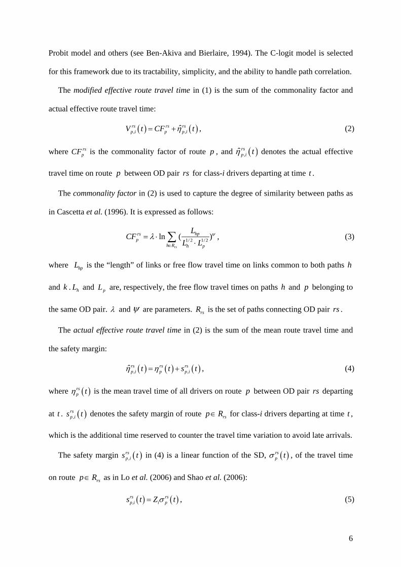
The modified effective route travel time in (1) is the sum of the commonality factor and
actual effective route travel time:
, ,ˆrs rs rs
p i p p iV t CF t , (2)
where rspCF
is the commonality factor of route p , and ,ˆ rs
p i t denotes the actual effective
travel time on route p between OD pair rs for class-i drivers departing at time t .
The commonality factor in (2) is used to capture the degree of similarity between paths as
in Cascetta et al. (1996). It is expressed as follows:
1/ 2 1/ 2
ln ( )rs
hprsp
h R h p
LCF
L L
, (3)
where hpL is the “length” of links or free flow travel time on links common to both paths h
and k . hL and pL are, respectively, the free flow travel times on paths h and p belonging to
the same OD pair. and are parameters. rsR is the set of paths connecting OD pair rs .
The actual effective route travel time in (2) is the sum of the mean route travel time and
the safety margin:
, ,ˆ rs rs rs
p i p p it t s t , (4)
where rsp t is the mean travel time of all drivers on route p between OD pair rs departing
at t . ,rsp is t denotes the safety margin of route rsp R for class-i drivers departing at time t ,
which is the additional time reserved to counter the travel time variation to avoid late arrivals.
The safety margin ,rsp is t in (4) is a linear function of the SD, rs
p t , of the travel time
on route rsp R as in Lo et al. (2006) and Shao et al. (2006):
,rs rsp i i ps t Z t , (5)

7
where iZ is the parameter representing the degree of the risk aversion of class-i drivers. The
larger is the value of iZ , the greater is the degree of the risk aversion of class-i drivers. In
particular, 0iZ if class-i drivers are risk-averse and tend to depart earlier to avoid late
arrivals; 0iZ if class-i drivers are risk-neutral and ignore rsp t when selecting routes. Of
course, iZ can also be related to the importance of the trip, i.e., by trip purpose (higher iZ
for more important trip and vice versa). The value of iZ can be calibrated using the survey
data. The details of the survey setting and calibration procedure can be found in Jackson and
Jucker (1982) but the SD is considered instead of the variance in this paper.
The motivation of (5) is that a higher degree of risk aversion implies a larger safety margin,
and a traveler reserves more additional time for a more uncertain route, where the uncertainty
is reflected by the SD of the route travel time.
The parameter iZ in (5) is related to the probability i that the actual travel time is not
greater than the actual effective route travel time:
,ˆ{ = } = ,rs rs rs rsp p i p i p iP C t t t Z t (6)
where ( )rspC t is the actual travel time on route p between OD pair rs when the traveler
departs at time t. The probability i can be regarded as the within budget time reliability,
where the budget is defined by the actual effective travel time. Then, a higher value of iZ
implies that the passenger is willing to have a higher probability of arriving on time or
equivalently the actual travel time not being greater than the actual effective travel time.
rsp t in (4) and rs
p in (5) are functions of all the route flows ,rsp if t f :
rsp
rsp
t
t
Φ f , (7)
where Φ represents a unique mapping yielding the means and SDs of route travel times from

8
route flows. This mapping is defined by the stochastic traffic flow model and the travel time
determination procedure. In this study, Φ is modeled by the proposed MC-SCTM, which
will be described in the next section.
Assume the perception errors in (1) follow the identical and independent Gumbel
distributions with mean zero and identical SD. The RSDUE route flow pattern can then be
formulated as:
, , , , , ,rs rs rsp i p i if t w t q t rs p t i , and (8)
,,
,
ˆexp( ( ( ) ))( ) , , , ,
ˆexp( ( ( ) ))
rs rsi p i prs
p i rs rsi k i k
k
t CFw t rs p t i
t CF
, (9)
where ,rs
p if t and ,rsp iw t are, respectively, the flow and proportion of class-i drivers on
route p between OD pair rs departing at time t ; rsiq t is the demand of class-i drivers
between OD pair rs at time t , which is assumed to be fixed; i is the dispersion parameter
representing the effective travel time perception variation of class-i drivers. A higher value of
i represents a better information quality received by the drivers. When i tends to infinity,
the flow pattern tends to be the reliability-based user equilibrium flow pattern. If iZ = 0, the
flow pattern becomes the dynamic stochastic user equilibrium flow pattern. If i tends to
infinity and iZ = 0, the flow pattern tends to be the dynamic user equilibrium flow pattern.
The MDS-SDUE-P is to find f to satisfy (3)-(9). Since ,rsp iw t
is a function of the path
flow ,rsp if t , this problem can be formulated as a fixed point problem:
,[ ]rs rsp i iw t q t f Y f , (10)
where ,rsp iw t is defined by
(3)-(5), (7), and (9). As (10) can be reformulated as a variational
inequality (VI), the existence and uniqueness of solutions for the proposed problem can be
analyzed by using the existence and uniqueness theorems for VIs. If the means and SDs of

9
route travel times are continuous of f , a solution exists to the proposed problem. The
uniqueness of the solution further requires , ,rs rs rs
p i p i if t w t q t F f to be strongly
monotone, which is almost unlikely in general cases.
3. THE MONTE-CARLO-BASED STOCHASTIC CELL TRANSMISSION MODEL
The proposed Monte-Carlo-based stochastic cell transmission model (MC-SCTM) is
developed from the cell transmission model (CTM) proposed by Daganzo (1994). The CTM
is a convergent numerical approximation scheme to the hydrodynamic model of Lighthill and
Whitham (1955) and Richards (1956). Daganzo’s CTM (1994) is originally developed for a
simple highway based on a trapezoidal flow-density relation, which includes the triangular
one as a special case. However, the CTM can be extended to consider general networks
(Daganzo, 1995a), general flow-density relations (Daganzo, 1995b), priority vehicles and
special lanes (Daganzo, 1997 and Daganzo et al., 1997) and lane-changing behavior (Laval
and Daganzo, 2006). In terms of formulation representation, the CTM can use either cell
occupancy (e.g., Daganzo, 1995a,b) or cell density (Daganzo, 1999; Muñoz et al., 2003) as
the state variable, where the cell occupancy is defined as the number of vehicles in a cell, and
the cell density is defined as the average number of vehicles in a cell per unit distance.
The CTM can capture traffic dynamics such as shockwaves, queues formation, queue
dissipation, and dynamic traffic interactions across multiple links (Lo and Szeto, 2002a, b).
However, the CTM requires dividing a link into many cells with equal lengths, leading to a
high computation burden. To reduce computation time, various modifications to the CTM
have been proposed. These modifications allow variable cell lengths (Ziliaskopoulos and Lee,
1997; Daganzo, 1999; Muñoz et al., 2003; Ishak et al., 2006; Szeto, 2008), and hence require
few cells and can reduce the computation burden. Nevertheless, their developments are based
on deterministic flow-density relations. The random evolution of traffic states due to

10
randomness in driving behavior, the changing weather conditions, etc. is not captured.
The stochastic cell transmission model (SCTM), proposed by Sumalee et al. (2010)
considers the random evolution of traffic states. This model extends the CTM by defining
parameters governing sending and receiving functions explicitly as random variables as well
as by specifying the dynamics of the basic model parameters of the FD including free flow
speed, backward wave speed, saturation flow rate, and jam density in each cell. The SCTM
employs a triangular flow-density relation and uses densities as state variables instead of cell
occupancies. Moreover, the SCTM allows variable cell lengths. The SCTM is shown to be
able to give a good estimate on the mean actual traffic flow on freeways (Sumalee et al.,
2010). However, the SCTM does not consider route choice and the First-In-First-Out (FIFO)
rule at diverges. Hence, the SCTM cannot be used to model traffic propagation in general
networks. In addition, the correlations between the model parameters between different cells
are not captured.
The proposed MC-SCTM considers route choice, FIFO, and the correlations between the
model parameters of trapezoidal flow-density relationships of various cells at the expense of
the increase in computation time. The MC-SCTM allows the parameters to be modeled by
any distribution with correlation between the model parameters to fit the observed data better.
The MC-SCTM relies on the Monte Carlo simulation (MCS) to generate traffic states for
network loading and collect travel time statistics from each network loading. The network
loading is done by the proposed modified CTM (M-CTM) which is extended from the
existing network version of the CTM (Daganzo, 1995) that use occupancies as state variables.
The M-CTM allows cells having unequal lengths regardless of actual free flow speed, and is
more suitable for large networks with random evolution of traffic states than the existing
network version of the CTM.
In the M-CTM, a highway is discretized into many cells and the study horizon is

11
discretized into many equal length intervals. The length of each cell is equal to the product of
the maximum free flow speed for that cell and the length of each time interval. Then, the flow
propagation equation of the M-CTM for a simple highway is the same as that of the CTM:
11 ,j j j jn n y y (11)
where the subscript j refers to cell j, and the subscript j-1 represents the cell upstream of j.
The variables jn and jy denote the number of vehicles in cell j and the actual
number of vehicles entering cell j at time , respectively. Basically, (11) states that the
number of vehicles in cell j at time 1 is equal to the number of vehicles in that cell at
time plus those entering minus those leaving.
As in the CTM, the M-CTM uses the Godunov scheme (see Godunov, 1959) to set the
actual number of vehicles entering cell j at time to be the minimum of the maximum
possible number of vehicles leaving the upstream cell j-1 at that time, 1jS , and the
maximum possible number of vehicles entering cell j at that time, jR :
1min , ,j j jy S R (12)
To account for non-uniform cell lengths, the M-CTM calculates 1jS and jR
based on the following:
min , , j
j j jj
NS Q n
d
and (13)
min , , ,j jj j j j
j j
w NR Q N n
v d
(14)
where jQ denotes the inflow capacity of cell j or the maximum number of vehicles that
can flow into cell j during time . jn and jN are, respectively, the occupancy of
cell j and the maximum number of vehicles that can be present in cell j (or the holding

12
capacity of cell j) at time . The latter equals the product of the number of lanes, the jam
density, and the length of the cell. jw and jv are, respectively, the backward wave
speed and the free flow speed of cell j during time . jd is the length of cell j. Equations
(13)-(14) assume that any cell j is made up of n “imaginary” standard cells connected in
series, where n is a positive integer and a standard cell is the shortest cell in the network.
According to (13), the sending flow of cell j is constrained by the inflow capacity, the cell
occupancy, and the holding capacity of the last “imaginary” standard cell of cell j. Equation
(14) states that the available capacity of cell j is the minimum of the inflow capacity of cell j,
the product of the vacant space j jN n and the factor j jw v that accounts
for the effect of shockwave on the vacant space in cell j , and the holding capacity of the first
“imaginary” standard cell embedded in cell j.
In a general network with many OD pairs, the general principle of (11)-(14) is still
applicable to the vehicle movements between cells. However, to maintain the intended routes
of vehicles and the FIFO property, the number of vehicles in each cell is disaggregated by
route (p) and by waiting time ( , modeled as a discrete time index). The route variable is
used to direct vehicles at merges and diverges. By tracking , the FIFO property is
maintained by ensuring that earlier arrivals (with a larger ) will leave sooner.
For a simple highway, the conservation of traffic flow leads to the following
, , 1 , , , ,( 1) ( ) ( ),j p j p j pn n y and (15)
1, ,1 , ,1 ,j p j pn y
(16)
where , ,j pn
denotes the number of vehicles in cell j at time on route p and enters the
cell at time 1 , and , ,j py denotes as the number of vehicles (on route p and that
has been waiting for time intervals) leaving cell j at time . Equation (15) states that the

13
remaining number of vehicles in cell j at time +1 (determined by the difference between
the number of vehicles in cell j at time minus those leaving) increases their waiting time
from to 1 . Equation (16) states that the vehicles enters cell j+1 at 1 .
If the minimum waiting time ja in cell j at time is known, then , ,j py in (15)
and (16) can be determined by:
, ,
, , , ,
if ,
if ,
0 if ,
j p j
j p j j p j
j
n a
y a n a
a
(17)
where ja
denotes the smallest integer equal to or greater than ja . Equation (17)
states that if the waiting time of any vehicle is longer than ja
, the vehicle advances
to the next cell; none of the vehicles leave cell j if their waiting time is less than ja ; and
lastly, for all the vehicles in cell j with waiting time ja
, only , ,j j pa n
of them leave the cell.
To avoid vehicles traveling at a speed higher than the free flow speed, according to the
Courant-Friedrichs-Levy condition (Courant et al., 1967), the minimum waiting time ja ,
or equivalently the minimum number of intervals required by a vehicle to stay in cell j, must
be at least equal to the minimum number of intervals required to leave cell j , jt :
j ja t . (18)
The latter depends on the length and actual free flow speed of the cell as follows:
max,
0
,j jj
j
d vt
d v
(19)
where jv and max, jv , respectively, denote the actual and maximum free flow speeds of cell

14
j with jv max, jv , and jv =
max, jv when there is no uncertainty for jv . jd and 0d ,
respectively, denote the lengths of cell j and the shortest cell. They represent the distance
traveled by a vehicle at the maximum free flow speed during one time interval. Equation (19)
states that jt is directly proportional to the length of cell j and inversely proportional to
the actual free flow speed jv . In the extreme case, when jd = 0d and jv =
max, jv ,
,j , the M-CTM is reduced to the CTM.
The M-CTM also has the following relationship:
, ,
j
j j pt p
n n
, and (20)
, ,j j pp
y y
. (21)
Equations (12)-(21) can be used to determine the traffic propagation for a simple highway
over time. Suppose the disaggregate occupancies , , , , ,j pn j p and the necessary
boundary conditions are known. Then, we can obtain ,jn j by (20). After that, by
solving the system of equations (12)-(14), (17), (19), (21), we can determine ja and
, ,j py simultaneously, which are used to compute , , 1( 1)j pn and 1, ,1 1 , ,j pn j p
through (15) and (16), respectively. The new disaggregate occupancies , , 1 , , ,j pn j p
can then be used to obtain the disaggregate occupancies for next time interval. This procedure
is repeated in the ascending order of .
Compared with Daganzo (1995), the new feature of the M-CTM is described by (13), (14),
(19), and (20). For general networks, the M-CTM still adopts the merge and diverge concepts
proposed in Daganzo (1995) but the maximum possible numbers of vehicles leaving and
entering a cell on each branch are determined by (13) and (14), respectively, and the
disaggregate cell occupancy on each branch is determined by (19) and (20).

15
The M-CTM discussed above is to determine the travel time given the path inflow kf for
one realization in the MC-SCTM. To obtain the means and SDs of route travel times, many
realizations are generated by the MCS. To reduce computation time, the MC-SCTM
incorporates the common random number MCS method and recursive formulas for
determining the means and SDs of route travel times. The algorithmic steps of the MC-
SCTM are as follows:
1.) Select the maximum number of samples for each iteration maxM . Set the sample
number 0m , the estimates of the means and SDs of route travel times
, , , ,0, 0, , ,rs rsp t m p t m rs p t .
2.) Set 1m m . Generate an observation mμ for free flow speed, backward wave speed,
jam density, and saturation flow for each cell at each time interval from the
predefined distributions.
3.) Load the path inflows kf into the cell network using the M-CTM.
4.) Deduce the cumulative inflow and outflow curves. Calculate the travel time
, , , , ,rs k mp t rs p t f μ using the procedure in Tong and Wong (2000), Lo and Szeto
(2002) or Long et al. (2010).
5.) Update the mean route travel time and the corresponding
SD based on
, , , 1
, , , , 1
,, , ,
rs k m rsp t p t mrs rs
p t m p t m rs p tm
f ω, and (22)
22
, , , , 1 , , , , 1
11 , , ,
1rs rs rs rsp t m p t m p t m p t mm rs p t
m
. (23)
6.) If maxm M , go to 2.). Otherwise, set rsp t =
max, ,rsp t M , and rs
p t = max, ,
rsp t M .
To sum up, given the path inflow kf , the MC-SCTM can calculate the occupancy of each
cell together with the means and SDs of route travel times.

16
4. THE SELF-REGULATED AVERAGING SOLUTION METHOD
The method of successive averages (MSA) was extensively used to solve the fixed point
problem during the past decades. This method relies on a predetermined step size for
guaranteeing convergence. However, the convergence speed of the MSA is slow due to two
reasons: 1) The predetermined step size is too large at some iterations such that the next
solution is even farther away from the optimal solution than the current one (i.e.,
overshooting occurs), and 2) When the current solution is close to the optimal solution, the
predetermined step size is too small and the convergence process is slowed down.
A self-regulated averaging method (SAM) was proposed by Liu et al. (2009) to deal with
the slow convergence problem, and was used to solve the deterministic-network stochastic
user equilibrium (SUE) problem. Nevertheless, to our best knowledge, this method has not
been used to solve stochastic network assignment problems yet. In this paper, we adopt this
method to solve our proposed stochastic problem, which relies on the Euclidean distances
( )k kf Y f in the two consecutive iterations to select an appropriate step size. If
( )k kf Y f 1 1( )k k f Y f , a step size larger than that of the MSA at iteration k will be
chosen to speed up the convergence process. Otherwise, a step size smaller than that of the
MSA at iteration k will be chosen to reduce the chance of overshooting.
Due to the sampling errors of MCS, the error estimate for each (major) iteration may not
be exact. Therefore, instead of just using the Euclidean distance at the current iteration k, we
use a simple moving average of the last three Euclidean distances as the convergence
measure. The detailed algorithm steps are as follows:
1.) Initialization: Set the number of major iterations 1k and the initial step size 0 1 .
Define parameters such as the maximum number of iterations maxk , the convergence
tolerance , the step size parameters and . Set the initial route flows 0f .

17
2.) Updating the mapping function: Based on kf , determine the means and SDs of route
travel times by the MC-SCTM. Calculate kY f .
3.) Checking convergence: Report results and stop if i) maxk k , or ii)
2
1( )
3
kj j j
j k
f Y f , 3k , where
2, ,Y( ) ( ( ) )k k rs rs rs
p i p i irs p i t
f t w t q t f f . (24)
4.) Step size determination: The self-regulated step size 1 /k ka , and k is updated by:
1 1 1
1 1 1
, 1, if ( ) ( ) ,
, 1, if ( ) ( ) .
k k k k k
k
k k k k k
f Y f f Y f
f Y f f Y f (25)
5.) Updating the flow pattern: 1 ( ( ) )k k k k k ka f f Y f f , 1k k and go to 2.)
Note that when 1 , the SAM becomes the MSA.
5. NUMERICAL STUDIES
Eight examples are set up to illustrate the properties of the problem and the performance of
the solution method. These examples are summarized in Table 1. For examples 1-5, 7 and 8,
a 10-cell network in Figure 2 is used. This network has one OD pair where cell 1 is the origin
cell and cell 10 is the destination cell. The basic settings for these examples are as follows:
Cell lengths: a) cells 3, 4, and 6: 5 miles; b) cell 7: 3 miles, and c) other cells: 1 mile;
The number of lanes: a) cells 5 and 8: 2; b) cells 3, 4, 6, and 7: 3; c) other cells: 6;
Convergence tolerance: = 0.01;
Length of a discretized time interval: 1 minute;
Sample size of the MCS: 1000;
Route choice parameters: 1.65Z , 1 0.05 ; = = 1;

18
Demand: a) level: 1800 veh/hr/lane; b) loading period: 1,15 ;
Parameters for the FD of each cell: symmetric triangular distributions with
a) Free flow speed: The maximum is 60 mph, and the minimum is 50 mph;
b) Backward wave speed: The maximum is -10 mph, and the minimum is -20 mph;
c) Jam density: The maximum is 240 veh/mile, and the minimum is 160 veh/mile;
d) Saturation flow: The maximum is 1800 veh/hr/lane, and the minimum is 1620
veh/hr/lane, except cells 6 - 8, where the minimum is 1080 veh/hr/lane.
With these settings, the lower route is shorter than the upper one, but has a larger SD and a
lower mean saturation flow.
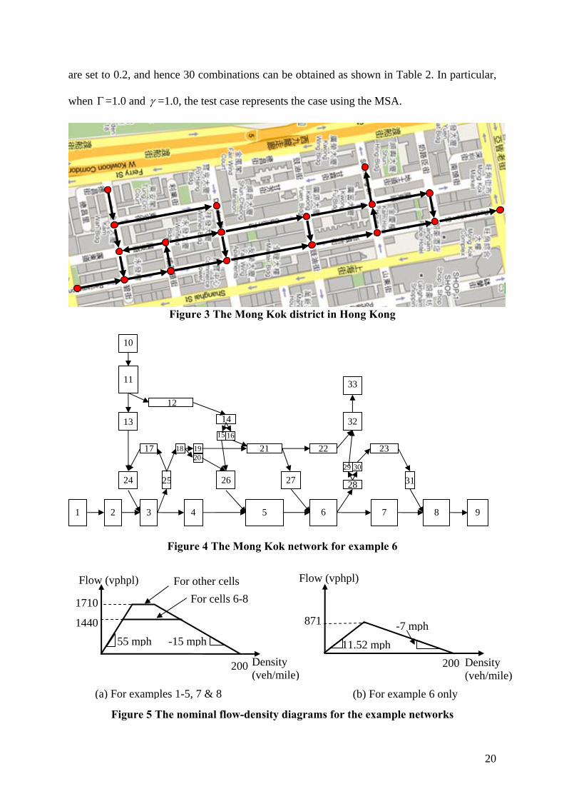
For example 6, the Mong Kok district (see Figure 3) is considered and modeled as shown
in Figure 4. The network has 4 OD pairs and 33 cells. The shortest and longest cells are 0.02
mile and 0.08 mile long, respectively. Each time interval is 5 seconds long. The rest of
parameter settings are similar to those for the small network, except the following:
Cell lengths: a) cells 5, 12, and 21: 0.08 mile; b) cells 6, 7, 8, 11, 22, and 23: 0.06 mile,
and c) cells 15, 16, 18, 19, 20, 29, and 30: 0.02 mile; d) other cells : 0.04 mile;
The numbers of lanes: a) cells 1 to 9: 3; b) cells 10, 11, 13, 14, 24, 26, 27, 28, 32, and 33:
2; c) other cells: 1;
Demand levels: OD pair 1-9: 960 veh/hr/lane; OD pair 10-9: 1080 veh/hr/lane, and OD
pairs 1-33 and 10-33: 720 veh/hr/lane;
Parameters for the FD of each cell: symmetric triangular distributions with
a) Free flow speed: The maximum is 14.4 mph, and the minimum is 8.64 mph;
b) Backward wave speed: The maximum is -6 mph, and the minimum is -8 mph.
The nominal fundamental diagrams for the two networks are shown in figure 5.
All examples were run on a computer with an Intel (R) Core(TM) 2 Duo T9400 2.53GHz
CPU and a 3GB RAM. Unless stated otherwise, each example is run for 20 times with

19
different seeds, and the average results are reported. Initially, the demand in each period is
evenly assigned to each path at the first iteration.
Table 1 Example setting
Figure 2 A ten-cell network for examples 1-5, 7 and 8
Example 1
This example is set up to illustrate the effect of the different combinations of and on
computation time and compare the performance between the SAM and the MSA. In this
example, is in the range from 1.0 to 2.0, while is in the range from 0.2 to 1.0, thereby
capturing the range recommended by Liu et al. (2006). The increments for these parameters
Example Network No. of classes N
Illustration Setting/ Remarks
1 10-cell network
1 Effects of and on computation time
Different combinations of and
2 10-cell network
1 Effect of on computation time
= 0.05, 0.1, 0.15, 0.2, 0.25
3 10-cell network
1 Effect of demand on computation time
Demand = 600, 900, 1200, 1500, 1800 veh/hr/lane
4 10-cell network
1 Effect of Z on computation time
Z = 0, 0.825, 1.65
5 10-cell network
varied Effect of the number of classes on computation time
N = 1, 2, and 3
6 Mong Kok Network
1 Computation performances of constant and varying sample size strategies
Change the sample size of MCS from 100 to 1000 at different convergence levels
7 10-cell network
1 Effect of the degree of risk aversion and on route choice
See below
8 10-cell network
2 Effect of information quality on the mean and SD of total system travel time
See below
1 2
3
6
4
7 8
9 10
5
20
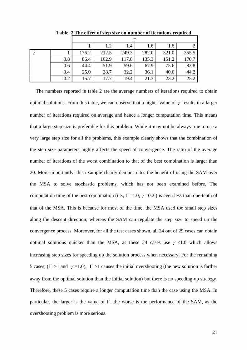
are set to 0.2, and hence 30 combinations can be obtained as shown in Table 2. In particular,
when =1.0 and =1.0, the test case represents the case using the MSA.
Figure 3 The Mong Kok district in Hong Kong
Figure 4 The Mong Kok network for example 6
Figure 5 The nominal flow-density diagrams for the example networks
18 19
9
2
3 4 5 6 7 8
10
12
15
11
14
17 20
22
25 26 31
33
1
13
24
30 29
23
28
32
21
27
16
1710
1440
-15 mph
Flow (vphpl)
Density (veh/mile)
200 200
871
Flow (vphpl)
55 mph
Density (veh/mile)
-7 mph
11.52 mph
(a) For examples 1-5, 7 & 8 (b) For example 6 only
For other cells
For cells 6-8
21
Table 2 The effect of step size on number of iterations required
1 1.2 1.4 1.6 1.8 2
1 176.2 212.5 249.3 282.0 321.0 355.5 0.8 86.4 102.9 117.8 135.3 151.2 170.7 0.6 44.4 51.9 59.6 67.9 75.6 82.8 0.4 25.0 28.7 32.2 36.1 40.6 44.2
0.2 15.7 17.7 19.4 21.3 23.2 25.2 The numbers reported in table 2 are the average numbers of iterations required to obtain
optimal solutions. From this table, we can observe that a higher value of results in a larger
number of iterations required on average and hence a longer computation time. This means
that a large step size is preferable for this problem. While it may not be always true to use a
very large step size for all the problems, this example clearly shows that the combination of
the step size parameters highly affects the speed of convergence. The ratio of the average
number of iterations of the worst combination to that of the best combination is larger than
20. More importantly, this example clearly demonstrates the benefit of using the SAM over
the MSA to solve stochastic problems, which has not been examined before. The
computation time of the best combination (i.e., =1.0, =0.2.) is even less than one-tenth of
that of the MSA. This is because for most of the time, the MSA used too small step sizes
along the descent direction, whereas the SAM can regulate the step size to speed up the
convergence process. Moreover, for all the test cases shown, all 24 out of 29 cases can obtain
optimal solutions quicker than the MSA, as these 24 cases use <1.0 which allows
increasing step sizes for speeding up the solution process when necessary. For the remaining
5 cases, ( >1 and =1.0), >1 causes the initial overshooting (the new solution is farther
away from the optimal solution than the initial solution) but there is no speeding-up strategy.
Therefore, these 5 cases require a longer computation time than the case using the MSA. In
particular, the larger is the value of , the worse is the performance of the SAM, as the
overshooting problem is more serious.

22
Example 2-Example 4
Examples 2-4 aim to illustrate the effect of parameters on computation time. For each
example, to avoid being smeared by other factors, we only vary one parameter value while
keeping other values fixed as those used in the basic setting. The best combination of and
(i.e., =1.0, =0.2.) is used to solve for solutions. The results are presented in Figures 6-
8. Figure 6 show that information quality has significant effect on computation time as
reflected by the average number of iterations required to get optimal solutions. According to
Figure 6, when increases from 0.05 to 0.25, (representing the case when the information
quality increases), the average number of iterations required increases nearly double. While
the exact increase of average computation time depends on the specific problem, the
increasing trend here agrees with the observation obtained by solving the SUE problem by
the MSA under various values of (see Sheffi, 1985), where the SAM is a variant of the
MSA. When is small, effective travel time is less important and the information quality
plays a more important role in determining the flow pattern. In the limiting case, when =0,
effective travel time is not used for determining the flow pattern.
10
15
20
25
30
35
0.05 0.10 0.15 0.20 0.25
Infomation quality
Average
number of iterations
Figure 6 Effects of information quality on computation time
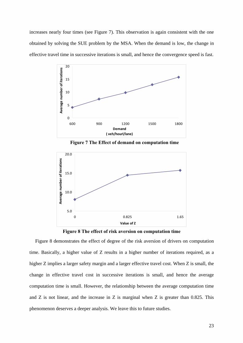
When the demand level increases from 600 veh/hr/lane to 1800 veh/hr/lane, the network
condition changes from free-flow to congested, and the average number of iterations
23
increases nearly four times (see Figure 7). This observation is again consistent with the one
obtained by solving the SUE problem by the MSA. When the demand is low, the change in
effective travel time in successive iterations is small, and hence the convergence speed is fast.
0
5
10
15
20
600 900 1200 1500 1800
Demand
( veh/hourl/lane)
Average
number of iterations
Figure 7 The Effect of demand on computation time
5.0
10.0
15.0
20.0
0 0.825 1.65
Value of Z
Average
number of iterations
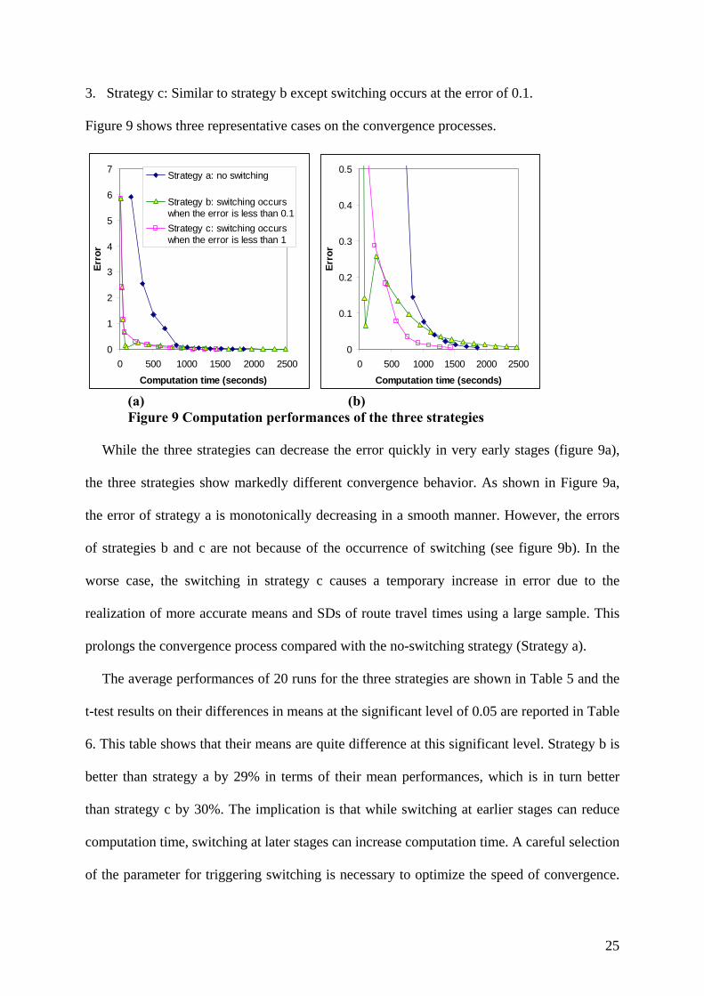
Figure 8 The effect of risk aversion on computation time
Figure 8 demonstrates the effect of degree of the risk aversion of drivers on computation
time. Basically, a higher value of Z results in a higher number of iterations required, as a
higher Z implies a larger safety margin and a larger effective travel cost. When Z is small, the
change in effective travel cost in successive iterations is small, and hence the average
computation time is small. However, the relationship between the average computation time
and Z is not linear, and the increase in Z is marginal when Z is greater than 0.825. This
phenomenon deserves a deeper analysis. We leave this to future studies.

24
Example 5
Table 3 compares the means and SDs of the computation times of the three cases (i.e., N =
1, N =2, and N = 3) over 20 runs. (Note that the average level of information quality and the
total demand of all the cases are the same in order to have a fair computation). The results of
the t-test on the difference in their means are shown in Table 4. The t-test shows that the
computation time for the case of N = 1 is smaller than that of N = 2 and that of N = 3 at the
significant level of 5 %, but the computation time for the case of N = 2 is greater than that of
N = 3 at the same significant level. These results indicate that increasing more variables in
the problem does not necessarily increase computation time.
Table 3 The computation times in seconds for various number of user classes
N=1 ( 1 0.1 ,
1,101 1800q t )
N=2( 1 0.05 , 2 0.15 ,
1,10 1,101 2 900q t q t )
N=3( 1 0.05 , 2 0.1 , 3 0.15 ,
1,10 1,10 1,101 2 3 600q t q t q t )
Mean 58.17 91.12 80.44SD 2.07 12.07 11.18
Table 4 t-tests on the difference in mean computation times Comparisons Difference in mean t-value Probability
Between the cases of N=1 and N=2 -32.95 -12.03 0.000 Between the cases of N=1 and N=3 -22.76 -8.76 0.000 Between the cases of N=2 and N=3 10.68 2.90 0.003
Example 6
This example aims to illustrate the computation performance of varying sample sizes during
the solution process. The Mong Kok network is used. Drivers are assumed to select paths
without cycles. Three strategies are considered:
1. Strategy a: A constant sample size of 1000 is used throughout the computation process.
2. Strategy b: A sample size of 100 is used initially. A sample is 1000 is used when the error
( )k kf Y f is less than 1.
25
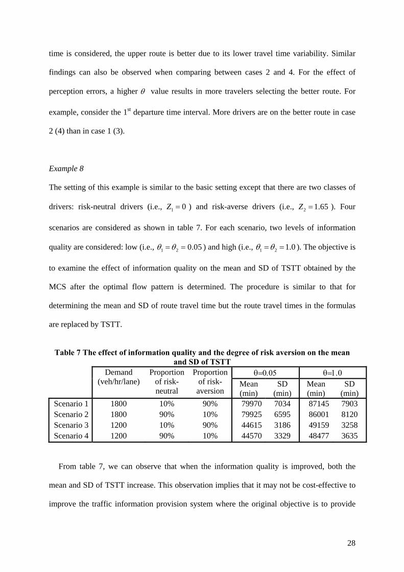
3. Strategy c: Similar to strategy b except switching occurs at the error of 0.1.
Figure 9 shows three representative cases on the convergence processes.
0
1
2
3
4
5
6
7
0 500 1000 1500 2000 2500
Computation time (seconds)
Err
or
Strategy a: no switching
Strategy b: switching occurswhen the error is less than 0.1
Strategy c: switching occurswhen the error is less than 1
0
0.1
0.2
0.3
0.4
0.5
0 500 1000 1500 2000 2500
Computation time (seconds)
Err
or
(a) (b) Figure 9 Computation performances of the three strategies
While the three strategies can decrease the error quickly in very early stages (figure 9a),
the three strategies show markedly different convergence behavior. As shown in Figure 9a,
the error of strategy a is monotonically decreasing in a smooth manner. However, the errors
of strategies b and c are not because of the occurrence of switching (see figure 9b). In the
worse case, the switching in strategy c causes a temporary increase in error due to the
realization of more accurate means and SDs of route travel times using a large sample. This
prolongs the convergence process compared with the no-switching strategy (Strategy a).
The average performances of 20 runs for the three strategies are shown in Table 5 and the
t-test results on their differences in means at the significant level of 0.05 are reported in Table
6. This table shows that their means are quite difference at this significant level. Strategy b is
better than strategy a by 29% in terms of their mean performances, which is in turn better
than strategy c by 30%. The implication is that while switching at earlier stages can reduce
computation time, switching at later stages can increase computation time. A careful selection
of the parameter for triggering switching is necessary to optimize the speed of convergence.

26
Nevertheless, in general, switching at earlier stages of the solution process can reduce
unnecessary sampling, as we only need a rough descent direction anyway. However, at later
stages, we need to have accurate mean and SD to find out an exact descent direction and an
optimal solution. Switching too late can prolong the convergence process.
Table 5 The computation times in seconds for various computation strategies
Strategy a Strategy b Strategy c Mean 1930.83 1500.01 2503.99
SD 83.74 269.03 332.31
Table 6 t-tests on the difference in mean computation times Difference in mean t-value Probability
Comparison between strategies a and b 430.82 6.84 0.000 Comparison between strategies a and c -573.16 -7.48 0.000 Comparison between strategies b and c -1003.99 -10.50 0.000
Example 7
To illustrate the effect of the degree of risk aversion and information quality on route choice,
four cases are set up: (1) 0.00, 0.05Z (risk-neutral drivers with poor information
quality), (2) 0.00, 0.10Z (risk-neutral drivers with better information quality), (3)
1.65, 0.05Z (risk-averse drivers with poor information quality), and (4)
1.65, 0.10Z (risk-averse drivers with better information quality).
The optimal result of each case is depicted in Figure 10.
In Figure 10, we can see that the four lines are distinct implying that different route choice
assumptions give significantly different equilibrium route flow proportions. For example, for
the 1st departure time interval, the difference in route flow proportions between cases 1 and 4
is about 8%. This observation further implies that the route choice assumption can greatly
affect the results of performance evaluation because most performance measures, e.g., total
system travel time (TSTT), highly depend on the flow proportions.

27
0.45
0.5
0.55
0.6
0.65
1 3 5 7 9 11 13 15
Departure time
Flow proportion of the
lower route
Case 1: Z=0.00, θ=0.05
Case 2: Z=0.00, θ=0.10
Case 3: Z=1.65, θ=0.05
Case 4: Z=1.65, θ=0.10
Figure 10 Proportions of drivers on the lower route
We can also observe that the best route changes with the departure time. When the route
flow proportions are above 0.5, the route is the best one. According to figure 10, for all cases,
the lower route (with a shorter mean travel time but a higher SD) is the best route only during
early periods. For cases 1 and 2 (i.e., risk-neutral drivers), the lower route is better in terms of
mean travel time in early periods. However, since the mean saturation flow on the lower
route is less than that of the upper route, the rate of increase of the mean travel time on the
lower route is faster than that of the upper one. Eventually, the mean travel time of the upper
route becomes better than that of the lower route. For cases 3 and 4 (i.e., risk-averse drivers),
similar to the case with risk-neutral drivers, the lower route is better initially in terms of
effective travel time, and then the mean and SD of travel time on this route become worse
than those on the upper route in later time periods. In particular, the increase of the SD of the
travel time on this route is because the queue formation occurs on this route and the
uncertainty of queue length accumulates over time.
The best route also varies from case to case. Consider the 9th departure time interval, the
proportion is greater (less) than 0.5 for case 1 (case 3), which means that the lower (upper)
route is better for case 1 (case 3). The implication is that when only mean travel time is
considered, the lower route is better as the mean is lower. However, when the effective travel
28
time is considered, the upper route is better due to its lower travel time variability. Similar
findings can also be observed when comparing between cases 2 and 4. For the effect of
perception errors, a higher value results in more travelers selecting the better route. For
example, consider the 1st departure time interval. More drivers are on the better route in case
2 (4) than in case 1 (3).
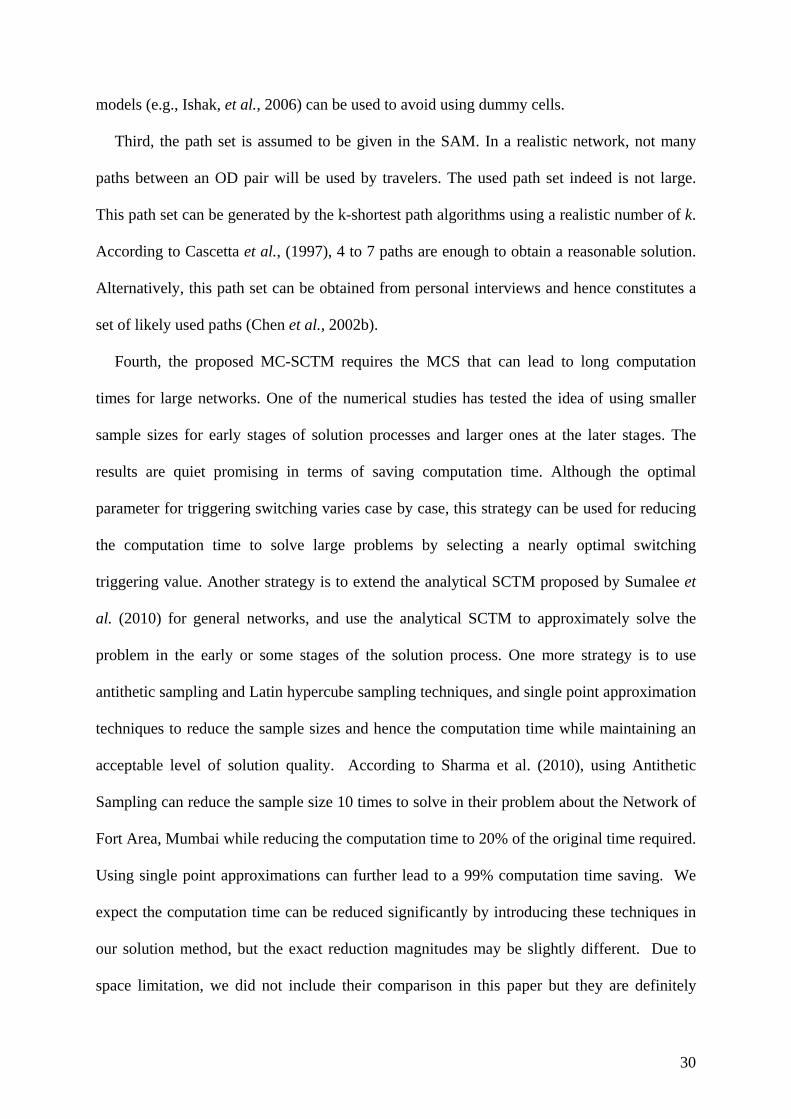
Example 8
The setting of this example is similar to the basic setting except that there are two classes of
drivers: risk-neutral drivers (i.e., 1 0Z ) and risk-averse drivers (i.e., 2 1.65Z ). Four
scenarios are considered as shown in table 7. For each scenario, two levels of information
quality are considered: low (i.e., 1 2 0.05 ) and high (i.e., 1 2 1.0 ). The objective is
to examine the effect of information quality on the mean and SD of TSTT obtained by the
MCS after the optimal flow pattern is determined. The procedure is similar to that for
determining the mean and SD of route travel time but the route travel times in the formulas
are replaced by TSTT.
Table 7 The effect of information quality and the degree of risk aversion on the mean
and SD of TSTT
Demand (veh/hr/lane)
Proportion of risk-neutral
Proportion of risk-aversion
Mean (min)
SD (min)
Mean (min)
SD (min)
Scenario 1 1800 10% 90% 79970 7034 87145 7903 Scenario 2 1800 90% 10% 79925 6595 86001 8120 Scenario 3 1200 10% 90% 44615 3186 49159 3258 Scenario 4 1200 90% 10% 44570 3329 48477 3635
From table 7, we can observe that when the information quality is improved, both the
mean and SD of TSTT increase. This observation implies that it may not be cost-effective to
improve the traffic information provision system where the original objective is to provide

29
better information for travelers to avoid passing through the congested area and reduce the
uncertainty of trip travel time due to unpredictable congestion. While the mean is increased
by around 9 % in all scenarios, the SD is increased by 2-23%, depending on scenarios. The
extent of increase in SD depends on both the driver composition and the demand level. When
there are more risk-neutral drivers as in scenarios 2 and 4, improving information quality
results a higher increase in the SD of TSTT, because more risk-neutral drivers will select the
route with a lower mean travel time but a higher travel time variability. On the other hand,
when the demand level is higher (i.e., Scenarios 1 and 2), the percentage increase of the SD
of TSTT is also higher, since a more congested network leads to more uncertainty in trip time.
6. IMPLEMENTATION ISSUES TO REALISTIC NETWORKS
When implementing the proposed fixed-point model (including the submodel, the MC-
SCTM) and the solution method to realistic networks, the following issues should be
considered. First, the proposed cell-based modeling requires the following two conditions to
be satisfied simultaneously: 1) The cell length must equal the maximum free flow speed
times the length of a discretized time interval, and 2) The lengths of longer cells must be
multiples of the length of the shortest cell. These two conditions will restrict the numbers of
discretized time intervals and cells used, and the lengths of each discretized time interval and
cell. Normally, short time intervals and short cells can satisfy these conditions. However,
these can increase the computation time as the number of cells and time intervals increase.
Second, one cell for a corridor should be considered to reduce the number of cells used.
However, if there are lane additions or lane drops within a link, more cells should be
considered for modeling a link for increasing the modeling accuracy at the expense of
increasing computation time. For modeling junctions, sometimes dummy cells are added to
apply the merge and diverge models proposed in Daganzo (1995). More general intersection
30
models (e.g., Ishak, et al., 2006) can be used to avoid using dummy cells.
Third, the path set is assumed to be given in the SAM. In a realistic network, not many
paths between an OD pair will be used by travelers. The used path set indeed is not large.
This path set can be generated by the k-shortest path algorithms using a realistic number of k.
According to Cascetta et al., (1997), 4 to 7 paths are enough to obtain a reasonable solution.
Alternatively, this path set can be obtained from personal interviews and hence constitutes a
set of likely used paths (Chen et al., 2002b).
Fourth, the proposed MC-SCTM requires the MCS that can lead to long computation
times for large networks. One of the numerical studies has tested the idea of using smaller
sample sizes for early stages of solution processes and larger ones at the later stages. The
results are quiet promising in terms of saving computation time. Although the optimal
parameter for triggering switching varies case by case, this strategy can be used for reducing
the computation time to solve large problems by selecting a nearly optimal switching
triggering value. Another strategy is to extend the analytical SCTM proposed by Sumalee et
al. (2010) for general networks, and use the analytical SCTM to approximately solve the
problem in the early or some stages of the solution process. One more strategy is to use
antithetic sampling and Latin hypercube sampling techniques, and single point approximation
techniques to reduce the sample sizes and hence the computation time while maintaining an
acceptable level of solution quality. According to Sharma et al. (2010), using Antithetic
Sampling can reduce the sample size 10 times to solve in their problem about the Network of
Fort Area, Mumbai while reducing the computation time to 20% of the original time required.
Using single point approximations can further lead to a 99% computation time saving. We
expect the computation time can be reduced significantly by introducing these techniques in
our solution method, but the exact reduction magnitudes may be slightly different. Due to
space limitation, we did not include their comparison in this paper but they are definitely

31
deserved to be further studied and compared comprehensively.
Fifthly, the proposed model requires a fairly accurate time-dependent OD matrix. If this
matrix is not accurate enough, one can consider extending the model to consider departure
time choice as well, as the simultaneous route and departure time choice model only requires
an OD matrix like the one for the static traffic assignment. The cost is to estimate the
desirable arrival time and desirable arrival time interval of travelers. For the peak hour traffic,
this information is not difficult to obtain from surveys. Alternatively, one can consider time-
dependent OD matrix with a larger discretized time interval and the demand for each larger
interval is assumed to be equally split into several smaller time intervals for network loading.
7. CONCLUDING REMARKS
This paper proposes the MDS-DUE-P considering the random evolution of traffic states, the
effect of travel time variation on route choice, and the effect of spatial queues. The proposed
problem consists of two components: traffic flow and route choice components. The traffic
flow component extends the SCTM proposed in Sumalee et al. (2010) to consider general
networks. The route choice component is described by the dynamic extension of the effective
travel time concept. The proposed problem is formulated as a fixed point problem and solved
by the SAM. Numerical examples are set up to illustrate the properties of the problem and
performance of the solution method. The key findings and implications are as follows:
1. Reducing perception errors on traffic conditions may not be able to reduce the uncertainty
of estimating system performance. This has a strong implication on providing better but
free traffic information to travelers, as providing better information requires investment
but the investment may not result in reducing the occurrence of the worse case
performance.
2. Using the SAM can get solutions much quicker compared to using the MSA in most cases.

32
Moreover, the combination of the values of the step size parameters highly affects the
speed of convergence. This implies that when the combination of the parameters is
wrongly chosen, the rate of convergence can be worse than that of the MSA.
3. A higher demand, a better information quality, or a higher degree of the risk aversion can
lead to a higher computation time.
4. More driver classes do not necessary results in a longer computation time.
5. Computation time can be greatly reduced by using small sample sizes in the early stage of
solution processes.
A discussion on the implementation issues of the proposed model and the SAM to realistic
networks is also provided.
This study opens many research directions. Firstly, to use the proposed model for real
applications, we need to calibrate the parameters and validate the models. This can be one
future research direction. Secondly, the effects of physical queues have been captured in the
proposed model. Yet, their impacts on travel time uncertainty have not been investigated.
Indeed, it is interesting and important to investigate if there is a propagation of travel time
uncertainty from one route to another, as the travel time uncertainty affects the route choice.
This investigation should be carried out in the future. Thirdly, this paper does not consider
departure time choice and stochastic travel demand. Including these two components into the
model framework should be an interesting research direction. Fourthly, multiple-pipe and
variational theories as well as the modeling theories for lane-changing behaviour and moving
bottlenecks (Daganzo and Laval, 2005; Daganzo, 2006; Leclercq, 2007) have not been
advanced to deal with large-scale network assignment applications which requires modeling
the traffic interaction at junctions and reasonably short computation time. Advancing these
theories can be another future research direction. Fifthly, antithetic sampling and Latin
hypercube sampling techniques and single point approximation techniques have not been

33
incorporated in the solution method. A comprehensive evaluation and comparison of using
these techniques for solving the proposed problem can be done in the future. Finally, the
proposed model can be applied to transport planning and management by extending it to a
bilevel model and solved the resultant model by heuristics such as tabu search (e.g., Fan and
Machemehl, 2008; Mohan Rao and Shyju, 2010), genetic algorithms (Adeli and Kumar,
1995a,b; Sarma and Adeli, 2000a,b, 2001, 2002; Kim and Adeli, 2001; Teklu et al., 2007;
Jiang and Adeli, 2008; Cheng and Yen, 2009; Kang et al., 2009; Ng et al., 2009; Zeferino, et
al., 2009; Lee and Wei, 2010; Al-Bazi and Dawood, 2010), and ant colony heuristics (e.g.,
Vitins and Axhausen, 2009).
ACKNOWLEDGEMENTS
This research is jointly sponsored by the project funded by the University Research
Committee of the University of Hong Kong under the grant No. 201001159008, the project
funded by the Hui Oi Chow Trust Fund under the grant No. 200902172003, and the project
supported by the Research Grants Council of the Hong Kong Special Administration Region
under grant project No. PolyU 5271/08E. The authors are grateful for the three anonymous
referees for their constructive comments. Special thanks should also go to the Performance
Measurement System (PeMS) which provides the traffic flow data.
REFERENCES
Abdel-Aty, M. A., Kitamura, R. & Jovanis, P. P. (1997), Using stated preference data for
studying the effect of advanced traffic information on drivers' route choice, Transportation
Research Part C, 5, 39-50.
Adeli, H. & Kumar, S. (1995a), Distributed genetic algorithms for structural optimization,
Journal of Aerospace Engineering, 8, 156-163.

34
Adeli, H. & Kumar, S. (1995b), Concurrent Structural Optimization on a Massively Parallel
Supercomputer, Journal of Structural Engineering, ASCE, 121, 1588-1597.
Al-Bazi, A. & Dawood, N. (2010), Developing crew allocation system for precast industry
using genetic algorithms, Computer-Aided Civil and Infrastructure Engineering, 25(8).
Ben-Akiva, M. & Bierlaire, M. (1999), Discrete choice methods and their applications to
short-term travel decisions, R. Hall (ed), Handbook of Transportation Science, Kluwer
Academic, Boston, USA, pp. 5-34.
Boel, R. & Mihaylova, L. (2006), A compositional stochastic model for real time freeway
traffic simulation, Transportation Research Part B, 40, 319-334.
Boyce, D. E., Ran, B. & Li, I. Y. (1999), Considering travelers’ risk-taking behavior in
dynamic traffic assignment, Transportation Networks: Recent Methodological Advances,
M.G.H. Bell (ed.), Elsevier, Oxford, pp. 67-81.
Carey, M. & McCartney, M. (2004), An exit-flow model used in dynamic traffic assignment,
Computers & Operations Research, 31, 1583-1602.
Cascetta, E., Nuzzolo, A., Russo, F. & Vitetta, A. (1996), A modified logit route choice
model overcoming path overlapping problems: specification and some calibration results
for interurban networks, J. B. Lesort (ed), Transportation and Traffic Theory, Pergamon,
New York, pp. 697-711.
Cascetta, E., Russo, F., & A. Vitetta. (1997), Stochastic user equilibrium assignment with
explicit path enumeration: comparison of models and algorithms, Proceedings of the 8th
International Federation of Automatic Control Symposium on Transportation Systems,
Chania, Greece, 1078-1084.
Chen, A., Ji, Z. W. & Recker, W. (2002a), Travel time reliability with risk-sensitive travelers,
Transportation Research Record, 1783, 27-33.
Chen, A., Lo, H. K. & Yang, H. (2002b), A self-adaptive projection and contraction
35
algorithm for the traffic assignment problem with path-specific costs, European Journal of
Operational Research, 135, 27-41.
Chen, C., Jia, Z. & Varaiya, P. (2001), Causes and cures of highway congestion, IEEE
Control Systems Magazine, 21, 26-33.
Cheng, T. M. & Yan, R. Z. (2009), Integrating messy genetic algorithms and simulation to
optimize resource utilization, Computer-Aided Civil and Infrastructure Engineering, 24,
401-415.
Chiabaut, N., Christine Buisson, C., Leclercq, L. 2009 Fundamental diagram estimation
through passing rate measurements in congestion, IEEE Transactions on Intelligent
Transportation Systems 10, 355-359.
Connors, R. D. & Sumalee, A. (2009), A network equilibrium model with travellers'
perception of stochastic travel times, Transportation Research Part B, 43, 614-624.
Courant, R. Friedrichs, K & Lewy, H. (1967) Über die partiellen Differenzengleichungen der
mathematischen Physik, Mathematische Annalen, 100, 32–74.
Daganzo, C. F. (1994), The cell transmission model- a dynamic representation of highway
traffic consistent with the hydrodynamic theory, Transportation Research Part B, 28, 269-
287.
Daganzo, C. F. (1995a), The cell transmission model, Part II: Network traffic, Transportation
Research Part B, 29, 79-93.
Daganzo, C. F. (1995b), A finite difference approximation for the kinematic wave model,
Transportation Research Part B, 29, 261-276.
Daganzo, C. F. (1997), A continuum theory of traffic dynamics for freeways with special
lanes, Transportation Research Part B, 31, 1997, 83-102.
Daganzo, C. F. (1999), The lagged cell transmission model, A. Cedar (ed.), Transportation
and Traffic Theory, Pergamon-Elsevier, New York, pp. 88-103.
36
Daganzo, C. F., Lin, W. H. & del Castillo, J. M. (1997), A simple physical principle for the
simulation of freeways with special lanes and priority vehicles, Transportation Research
Part B, 31, 105-125.
Daganzo, C. F. & Laval, J. A. (2005), On the numerical treatment of moving bottlenecks,
Transportation Research Part B, 39, 31-46
Daganzo, C. F. (2006), On the variational theory of traffic flow: well-posedness, duality and
applications, Networks and Heterogeneous Media, 1, 601-619
Fan, W. & Machemehl, R. B. (2008), Tabu search strategies for the public transportation
network optimizations with variable transit demand, Computer-Aided Civil and
Infrastructure Engineering, 23, 502-520.
Geistefeldt, J. & Brilon, W. (2009), A comparative assessment of stochastic capacity
estimation methods, Lam et al. (eds), Transportation and Traffic Theory 2009: Golden
Jubilee, Springer, London, U.K., pp. 583-602.
Godunov, S. K. (1959), A difference scheme for numerical solution of discontinuous solution
of hydrodynamic equations, Math. Sbornik, 47, 271-306
Ishak, S., Alecsandru, C. & Seedah, D. (2006), Improvement and evaluation of the cell-
transmission model for operational analysis of traffic networks: freeway case study,
Transportation Research Record, 1965, 171-182.
Jackson, W. B. & Jucker, J. V. (1982), An empirical study of travel time variability and travel
choice behavior, Transportation Science, 16, 460-475.
Jiang, X. & Adeli, H. (2008), Neuro-genetic algorithm for nonlinear active control of highrise
buildings, International Journal for Numerical Methods in Engineering, 75, 770-786.
Kang, M. W., Schonfeld, P. & Yang, N. (2009), Prescreening and repairing in a genetic
algorithm for highway alignment optimization, Computer-Aided Civil and Infrastructure
Engineering, 24, 109-119.

37
Kim, H. & Adeli, H. (2001), Discrete cost optimization of composite floors using a floating
point genetic algorithm, Engineering Optimization, 33, 485-501.
Kim, T., & Zhang, H. (2008), A stochastic wave propagation model, Transportation
Research Part B, 42, 619-634.
Lam, W. H. K., Shao, H. & Sumalee, A. (2008), Modeling impacts of adverse weather
conditions on a road network with uncertainties in demand and supply, Transportation
Research Part B, 42, 890-910.
Laval, J. & Daganzo, C. F. (2006), Lane changing in traffic streams, Transportation Research
Part B, 40, 251-264.
Lee, Y. & Wei, C. H. (2010), A computerized feature selection using genetic algorithms to
forecast freeway accident duration times, Computer-Aided Civil and Infrastructure
Engineering, 25, 132-148.
Leclercq, L. (2007), Bounded acceleration close to fixed and moving bottlenecks,
Transportation Research Part B, 41, 309-319.
Lighthill, M. J. & Whitham, G. B. (1955), On kinematic waves (II): A theory of traffic flow
on long crowded roads, Proc. Roy. Soc., A. 229, 281-345.
Liu, H. X., Ban, X., Ran, B. & Mirchandani, P. (2002), Analytical dynamic traffic assignment
model with probabilistic travel times and perceptions, Transportation Research Record,
1783, 125-133.
Liu, H. X., He, X. Z. & He, B. S. (2009), Method of successive weighted averages (MSWA)
and self-regulated averaging schemes for solving stochastic user equilibrium problem,
Networks & Spatial Economics, 9, 485-503.
Lo, H. K. & Chen, A. (2000), Traffic equilibrium problem with route-specific costs:
formulation and algorithms, Transportation Research Part B, 34, 493-513.
Lo, H. K., Luo, X. W. & Siu, B. W. Y. (2006), Degradable transport network: travel time

38
budget of travelers with heterogeneous risk aversion, Transportation Research Part B, 40,
792-806.
Lo, H. K. & Szeto, W. Y. (2002a), A cell-based variational inequality formulation of the
dynamic user optimal assignment problem, Transportation Research Part B, 36, 421-443.
Lo, H. K. & Szeto, W. Y. (2002b), A cell-based dynamic traffic assignment model:
formulation and properties, Mathematical and Computer Modelling, 35, 849-865.
Long, J. C., Gao, Z. Y. & Szeto W. Y. (2010), Discretised link travel time models based on
cumulative flows: formulations and properties, Transportation Research Part B, accepted
Mohan Rao, A. R. & Shyju, P. P. (2010), A meta-heuristic algorithm for multi-objective
optimal design of hybrid laminate composite structures, Computer-Aided Civil and
Infrastructure Engineering, 25, 149-170.
Muñoz, L., Sun, X., Horowitz, R. & Alvarez, L. (2003), Traffic density estimation with the
cell transmission model, Proceedings of the American Control Conference, 3750-3755.
Newell, G. F. (1993), A simplified theory of kinematic waves in highway traffic, Parts I – III,
Transportation Research Part B, 27, 281-313.
Ng, M. W., Lin, D. Y. & Waller, S. T. (2009), Optimal long-term infrastructure maintenance
planning accounting for traffic dynamics, Computer-Aided Civil and Infrastructure
Engineering, 24, 459-469.
Ngoduy, D. (2009), Multiclass first order model using stochastic fundamental diagrams,
Transportmetrica, in press.
Nie, X. J. & Zhang, H. M. (2005a), A comparative study of some macroscopic link models
used in dynamic traffic assignment, Networks & Spatial Economics, 5, 89-115.
Nie, X. J. & Zhang, H. M. (2005b), Delay-function-based link models: their properties and
computational issues, Transportation Research Part B, 39, 729-751.
Peeta, S. & Zhou, C. (2006), Stochastic quasi-gradient algorithm for the off-line stochastic

39
dynamic traffic assignment problem, Transportation Research Part B, 40, 179-206.
Richards, P. I. (1956), Shockwaves on the highway, Operations Research, 4, 42-51.
Sarma, K. C. & Adeli, H. (2000a), Fuzzy genetic algorithm for optimization of steel
structures, Journal of Structural Engineering, ASCE, 126, 596-604.
Sarma, K. C. & Adeli, H. (2000b), Fuzzy discrete multicriteria cost optimization of steel
structures, Journal of Structural Engineering, ASCE, 126, 1339-1347.
Sarma, K. C. & Adeli, H. (2001), Bi-level parallel genetic algorithms for optimization of
large steel structures, Computer-Aided Civil and Infrastructure Engineering, 16, 295-304.
Sarma, K. C. & Adeli, H. (2002), Life-cycle cost optimization of steel structures,
International Journal for Numerical Methods in Engineering, 55, 1451-1462.
Sharma, S., Mathew T. V. & Ukkusuri, S. V. (2010), Approximation techniques for
transportation network design problem under demand uncertainty, Journal of Computing
in Civil Engineering, accepted.
Shao, H., Lam, W. H. K. & Tam, M. L. (2006), A reliability-based stochastic traffic
assignment model for network with multiple user classes under uncertainty in demand,
Networks & Spatial Economics, 6, 173-204.
Shao, H., Lam, W. H. K., Tam, M. L. & Yuan, X. M. (2008), Modelling rain effects on risk-
taking behaviours of multi-user classes in road networks with uncertainty, Journal of
Advanced Transportation, 42, 265-290.
Siu, B. W. Y. & Lo, H. K. (2008), Doubly uncertain transportation network: Degradable
capacity and stochastic demand, European Journal of Operational Research, 191, 166-
181.
Sheffi, Y. (1985), Urban Transportation Networks: Equilibrium Analysis with Mathematical
Programming Methods. Prentice-Hall, Inc., Englewood Cliffs, New Jersey.
Sumalee, A., Zhong, R. X., Pan, T. L. & Szeto, W. Y. (2010), Stochastic cell transmission

40
model (SCTM): a stochastic dynamic traffic model for traffic state surveillance and
assignment, Transportation Research Part B, submitted.
Szeto, W. Y. (2008), Enhanced lagged cell-transmission model for dynamic traffic
assignment, Transportation Research Record, 2085, 76-85.
Szeto, W. Y. & Lo, H. K. (2005), The impact of Advanced Traveler Information Services on
travel time and schedule delay costs, Journal of Intelligent Transportation Systems:
Technology, Planning, and Operations, 9, 47-55.
Szeto, W. Y. & Lo, H. K. (2006), Dynamic traffic assignment: properties and extensions,
Transportmetrica, 2, 31-52.
Szeto, W. Y., Solayappan, M. & Jiang, Y. (2011), Reliability-based transit assignment for
congested stochastic transit networks, Computer-Aided Civil and Infrastructure
Engineering, 26(4).
Teklu, F., Sumalee, A. & Watling, D. (2007), A genetic algorithm for optimizing traffic
control signals considering routing, Computer-Aided Civil and Infrastructure Engineering,
22, 31-43.
Tong, C. O. & Wong, S. C. (2000), A predictive dynamic traffic assignment model in
congested capacity-constrained road networks, Transportation Research Part B, 34, 625-
644.
Vitins, B. J. & Axhausen, K. W. (2009), Optimization of large transport networks using the
ant colony heuristic, Computer-Aided Civil and Infrastructure Engineering, 24, 1-14.
Yin, Y. F., Lam, W. H. K. & Ieda, H. (2004), New technology and the modeling of risk-
taking behavior in congested road networks, Transportation Research Part C, 12, 171-
192.
Zeferino, J. A., Antunes, A. P. & Cunha, M. C. (2009), An efficient simulated annealing
algorithm for regional wastewater systems planning, Computer-Aided Civil and

41
Infrastructure Engineering, 24, 359-370.
Ziliaskopoulos, A. K. & Lee, S. (1997), A cell transmission based assignment-simulation
model for integrated freeway/surface street systems, Transportation Research Record,
1701, 12-23.
Zhou, Z. & Chen, A. (2008), Comparative analysis of three user equilibrium models under
stochastic demand, Journal of Advanced Transportation, 42, 239-263.


![Computer Engineering - USC Viterbi | Ming Hsieh Department ...ceng.usc.edu/techreports/1992/Silvester CENG 92-21.pdfNeuts' versatile Markov process [17], is a doubly stochastic Poisson](https://static.fdocuments.us/doc/165x107/60e721915eeab34ae2240965/computer-engineering-usc-viterbi-ming-hsieh-department-cenguscedutechreports1992silvester.jpg)

