A Cavendish Quantum Mechanics Primer€¦ · of quantum mechanics by solving phenomena such as how...

A Cavendish Quantum Mechanics Primer

M. Warner & A. C. H. CheungUniversity of Cambridge

Periphyseos Press

PERIPHYSEOS PRESS

Cambridge

Cavendish LaboratoryJ. J. Thomson Avenue, Cambridge CB3 0HE, UK

Published in the United Kingdom by Periphyseos Press, Cambridgewww.periphyseos.org.uk

Information on this title is available at: www. avendish-quantum.org.uk

c©M. Warner and A. C. H. Cheung 2012

This publication is in copyright. Subject to statutory exception and to theprovisions of relevant collective licensing agreements, no reproduction ofany part may take place without the written permission of Periphyseos

Press.

First published 2012

Printed in the United Kingdom at the University Press, Cambridge

Typeset by the authors in LATEX

A catalogue record for this publication is available from the British Library

ISBN 978-0-9572873-0-3 Paperback

used with kind permission of copyright owner M. J. Rutter.

Contents

Preface v

Acknowledgements . . . . . . . . . . . . . . . . . . . . . . . . . . . viiTeaching resources . . . . . . . . . . . . . . . . . . . . . . . . . . . viiiSymbols . . . . . . . . . . . . . . . . . . . . . . . . . . . . . . . . . ix

1 Preliminaries 1

1.1 Moving from classical to quantum . . . . . . . . . . . . . . . 1Quantum mechanics and probability in 1-D . . . . . . . . . . 2Uncertainty . . . . . . . . . . . . . . . . . . . . . . . . . . . . 2Measurement and duality . . . . . . . . . . . . . . . . . . . . 3Potentials . . . . . . . . . . . . . . . . . . . . . . . . . . . . . . 5Quantum mechanics in the world around us . . . . . . . . . 8

1.2 Mathematical preliminaries . . . . . . . . . . . . . . . . . . . 9Probability . . . . . . . . . . . . . . . . . . . . . . . . . . . . . 10Essential functions . . . . . . . . . . . . . . . . . . . . . . . . 11Calculus — differentiation . . . . . . . . . . . . . . . . . . . . 12Calculus — integration . . . . . . . . . . . . . . . . . . . . . . 14

Integration by parts . . . . . . . . . . . . . . . . . . . 16Differential equations . . . . . . . . . . . . . . . . . . . . . . . 18

Simple harmonic motion . . . . . . . . . . . . . . . . . 18Exponentially decaying motion . . . . . . . . . . . . . 21Interference of waves . . . . . . . . . . . . . . . . . . . 22Waves on a stretched string . . . . . . . . . . . . . . . 22

Qualitative analysis . . . . . . . . . . . . . . . . . . . . . . . . 24

i

ii

Vectors . . . . . . . . . . . . . . . . . . . . . . . . . . . . . . . 261.3 Summary . . . . . . . . . . . . . . . . . . . . . . . . . . . . . . 291.4 Additional problems . . . . . . . . . . . . . . . . . . . . . . . 29

2 Schrödinger’s equation 31

2.1 Observables and operators . . . . . . . . . . . . . . . . . . . . 31Eigenfunctions and eigenvalues . . . . . . . . . . . . . . . . . 33

2.2 Some postulates of quantum mechanics . . . . . . . . . . . . 352.3 The infinite square well potential . . . . . . . . . . . . . . . . 36

Quantisation . . . . . . . . . . . . . . . . . . . . . . . . . . . . 37Kinetic energy and the wavefunction . . . . . . . . . . . . . . 38

2.4 Confinement energy . . . . . . . . . . . . . . . . . . . . . . . 39Heisenberg meets Coulomb . . . . . . . . . . . . . . . . . . . 40Einstein meets Heisenberg and Coulomb . . . . . . . . . . . 42Mass effects in localisation . . . . . . . . . . . . . . . . . . . . 43Observation of quantum effects . . . . . . . . . . . . . . . . . 45

2.5 Summary . . . . . . . . . . . . . . . . . . . . . . . . . . . . . . 472.6 Additional problems . . . . . . . . . . . . . . . . . . . . . . . 47

3 Classically forbidden regions 49

3.1 The finite square well potential . . . . . . . . . . . . . . . . . 49Matching wavefunctions . . . . . . . . . . . . . . . . . . . . . 51The quantum states of the finite well . . . . . . . . . . . . . . 51

3.2 Harmonic potentials . . . . . . . . . . . . . . . . . . . . . . . 54The classical harmonic oscillator . . . . . . . . . . . . . . . . 55The quantum harmonic oscillator . . . . . . . . . . . . . . . . 56


4 Foundations of quantum mechanics 63

4.1 Complex numbers . . . . . . . . . . . . . . . . . . . . . . . . . 63Complex exponentials . . . . . . . . . . . . . . . . . . . . . . 65Hyperbolic functions . . . . . . . . . . . . . . . . . . . . . . . 67

4.2 Foundations . . . . . . . . . . . . . . . . . . . . . . . . . . . . 68Two slit experiment . . . . . . . . . . . . . . . . . . . . . . . . 69Momentum operator . . . . . . . . . . . . . . . . . . . . . . . 71Other formulations of quantum mechanics . . . . . . . . . . 72

4.3 Expectation values . . . . . . . . . . . . . . . . . . . . . . . . 73Energy eigenstates . . . . . . . . . . . . . . . . . . . . . . . . 73Superposition of eigenstates . . . . . . . . . . . . . . . . . . . 75

iii

4.4 Particle currents . . . . . . . . . . . . . . . . . . . . . . . . . . 77Currents onto steps . . . . . . . . . . . . . . . . . . . . . . . . 77


5 Space and time 85

5.1 Partial differentiation . . . . . . . . . . . . . . . . . . . . . . . 86Integration in more than 1-D . . . . . . . . . . . . . . 87

5.2 Further postulates of quantum mechanics . . . . . . . . . . . 885.3 Potentials in higher dimensions . . . . . . . . . . . . . . . . . 89

2-D infinite square well potential . . . . . . . . . . . . 89Free and bound motion together — nanowires . . . . 902-D free motion with a 1-D step . . . . . . . . . . . . . 92

Quantising a string . . . . . . . . . . . . . . . . . . . . . . . . 965.4 The dynamics of quantum states . . . . . . . . . . . . . . . . 985.5 Summary . . . . . . . . . . . . . . . . . . . . . . . . . . . . . . 1005.6 Outlook . . . . . . . . . . . . . . . . . . . . . . . . . . . . . . . 1015.7 Additional problems . . . . . . . . . . . . . . . . . . . . . . . 1025.8 Suggestions for further reading . . . . . . . . . . . . . . . . . 105

Index 107

v

PREFACE

This primer, starting with a platform of school mathematics, treats quan-tum mechanics “properly”. You will calculate deep and mysterious ef-fects for yourself. It is decidedly not a layman’s account that describesquantum mechanical phenomena qualitatively, explaining them by anal-ogy where all attempts at analogy must fail. Nor is it an exhaustive text-book; rather this brief student guide explains the fundamental principlesof quantum mechanics by solving phenomena such as how quantum par-ticles penetrate classically forbidden regions of space, how particle motionis quantised, how particles interfere as waves, and many other completelynon-intuitive effects that underpin the quantum world. The mathematicsneeded is mostly covered in the AS (penultimate) year at school. So takeheart! The quantum mechanics you will see may look formidable, but it isall accessible with your existing skills and with practice.

Chapters 1–3 require differentiation, integration, trigonometry and thesolution of two types of differential equations met at school. The only spe-cial function that arises is the exponential, which is also at the core of schoolmathematics. We revise this material. In these chapters we cover quanti-sation, confinement to potential wells, penetration into forbidden regions,localisation energy, atoms, relativistic pair production, and the fundamen-tal lengths of physics. Exercises appear throughout the notes. It is vitalto solve them as you proceed. They will make physics an active subjectfor you, rather than the passive knowledge gained from popular sciencebooks. Such problem solving will transform your fluency and competencein all of the mathematics and physics you study at school and the first yearsat university. Especially, the gained confidence in mathematics will under-pin further studies in any science; in any event, mathematics is the naturallanguage of physics.

Chapter 4 needs complex numbers. It introduces the imaginary numberi =√−1, something often done in the last year at school. Armed with i,

you will see that quantum mechanics is essentially complex, that is, it in-volves both real and imaginary numbers. Waves, so central to quantummechanics, also require revision. We shall then deal with free particles andtheir currents, reflection from and penetration of steps and barriers, flowof electrons along nano-wires and related problems. Calculating these phe-nomena precisely will consolidate your feeling for i, and for the complexexponentials that arise, or introduce you first to the ideas and practice inadvance, if you are reading them a few months early. Finally, Chapter 5introduces partial derivatives which are not generally done at school, but

vi

which are central to the whole of physics. They are a modest generalisa-tion of ordinary derivatives to many variables. Chapter 5 opens the wayto quantum dynamics and to quantum problems in higher dimensions. Werevisit quantum dots and nano wires more quantitatively. Chapters 4 and5 are more advanced and will take you well into a second-year universityquantum mechanics course.

Some readers will find Chapters 4 and 5 challenging at first. Physicsis an intellectually deep and difficult subject, wherein rests its attraction tothe ambitious student. While moving from exposure-level treatments to thereal edifice of physics, think of Alexander Pope

A little learning is a dangerous thing;drink deep, or taste not the Pierian spring:there shallow draughts intoxicate the brain,and drinking largely sobers us again.

Alexander Pope (1688–1744)from “An Essay on Criticism”, 1709

Physics is a linear subject; you will need the building blocks of mechanicsand mathematics to advance to quantum mechanics, statistical mechanics,electromagnetism, fluid mechanics, relativity, high energy physics and cos-mology. This book takes serious steps along this path of university physics.Towards the end of school, you already have the techniques needed to startthis journey; their practice here will help you in much of your higher math-ematics and physics. We hope you enjoy a concluding exercise, quantisingthe string — a first step towards quantum electrodynamics.

Mark Warner & Anson CheungCavendish Laboratory, University of Cambridge.June, 2012

vii

ACKNOWLEDGEMENTS

We owe a large debt to Robin Hughes, with whom we have extensivelydiscussed this book. Robin has read the text very closely, making great im-provements to both the content and its presentation. He suggested much ofthe challenging physics preparation of chapter 1. Robin and Peter Sammuthave been close colleagues in The Senior Physics Challenge, from whichthis primer has evolved. Peter too made very helpful suggestions and wasalso most encouraging over several months. Both delivered some quantummechanics to advanced classes in their schools, using our text. We wouldbe lost without their generosity and without their deep knowledge of bothphysics and of school students. Peter also shaped ACHC’s early physicsexperiences.

Quantum mechanics is a counter-intuitive subject and we would liketo thank Professor David Khmelnitskii for stimulating discussions and forclarification of confusions; MW also acknowledges similar discussions withProfessor J.M.F. Gunn, Birmingham University. We are most grateful to DrMichael Rutter for his indispensible computing expertise. Dr Dave Greenhas been invaluable in his support of our pedagogical aims with the SPCand this book, where he has assisted in clarifying our exposition. We alsothank colleagues and students who read our notes critically: Dr MichaelSutherland, Dr Michael Rutter; Georgina Scarles and Avrish Gooranah.Generations of our departmental colleagues have refined many of the prob-lems we have drawn upon in this primer. We mention particularly the workof Professor Bryan Webber. Of course, any slips in our new problems arepurely our responsibility.

ACHC thanks Trinity College for his Fellowship.The Ogden Trust was a major benefactor of the SPC over many years of

the project. The wider provision of these kinds of notes for able and ambi-tious school students is one of our goals that has been generously supportedby the Trust throughout.

viii

TEACHING RESOURCES

This primer grew from lecture notes written for the Senior Physics Chal-lenge (SPC), the schools physics development project of the Cavendish Lab-oratory, University of Cambridge. We aim to make it as widely available aspossible to school and university students alike: chapter 1 can be seen asa resource of problems and as an assembly of skills needed for Oxbridgeentry tests and interviews. The coincidence of this function with that ofpreparing for university level quantum mechanics is not accidental — flu-ency and confidence in its material is also needed for continuing study.Practice over a period will be required for the mastery of chapter 1, but thematerial is not advanced. It is then required for the remainder of the bookand in all higher physics. Chapters 2 and 3 would offer further practicefor fluency while exploring the wonders of quantum mechanics. Chapters2–5 form the core of our first two years of quantum mechanics teaching inCambridge.

Chapter 1 is freely downloadable at this primer’s website1 and at theSenior Physics Challenge website2.

Please consult THE PERIPHYSEOS PRESS3 for very substantial price re-ductions for group or bulk orders of this primer.

THE PERIPHYSEOS PRESS derives its name from Greek“peri” = “about, concerning”, and “physeos” = “(of) na-ture” — the same root as physics itself. The Press aims tomake texts on natural sciences easily and cheaply avail-able to students. The crocodile symbol ( c© M.J. Rutter),commissioned for the Cavendish Laboratory by the greatRussian physicist Kapitza, is thought to be a reference toLord Rutherford, the then Cavendish Professor.

AN INSTRUCTOR’S MANUAL2 is available to teachers asa companion to the primer. It has full solutions to all theproblems of the text and solved problems that go beyond the text itself.Points of difficulty, subtlety and extension are also discussed in the manual.

We would be grateful for suggestions for further material, or being madeaware of typographical and other errors that readers might find in the text.Please contact us via the Primer’s website.

1www. avendish-quantum.org.uk

2www-sp .phy. am.a .uk

3www.periphyseos.org.uk

SYMBOLS ix

Mathematical symbols and notation; Physical quantities

Greek symbols with a few capital forms (alphabetical order is left to right,then top to bottom):

α alpha β beta γ Γ gamma δ ∆ delta ǫ epsilonζ zeta η eta θ Θ theta ι iota κ kappaλ lambda µ mu ν nu ξ Ξ xi o omicronπ Π pi ρ rho σ Σ sigma τ tau υ Υ upsilonφ Φ phi χ chi ψ Ψ psi ω Ω omega ∇ nabla

Miscellaneous symbols and notation:

For (real) numbers a and b with a < b, the open interval (a, b) is the set of(real) numbers satisfying a < x < b. The corresponding closed interval isdenoted [a, b], that is, a ≤ x ≤ b.

∈ means “in” or “belonging to”, for example, the values of x ∈ (a, b).

∼ means “of the general order of” and “having the functional dependenceof”, for instance f (x, y) ∼ x sin(y).

∝ means “proportional to” f (x, y) ∝ x in the above example (there is morebehaviour not necessarily displayed in a ∝ relation).

〈(. . . )〉means the average of the quantity (. . . ); see Section 1.2.

∂/∂x means the partial derivative (of a function) with respect to x, otherindependent variables being held constant; see Section 5.1.

|. . .| means “the absolute value of”. For complex numbers, it is more usualto say “modulus of”.

Physical quantities:

Constant Symbol Magnitude Unit

Planck’s constant/2π h 1.05× 10−34 J s

Charge on electron e 1.6× 10−19 C

Mass of electron me 9.11× 10−31 kg

Mass of proton mp 1.67× 10−27 kg

Speed of light c 3.00× 108 m s−1

Bohr radius aB = 4πǫ0 h2/(mee2) 53.0× 10−12 m

Permittivity free space ǫ0 8.85× 10−12 F m−1

CHAPTER

1Preliminaries — some

underlying quantum ideas

and mathematical tools

1.1 Moving from classical to quantum

Wavefunctions, probability, uncertainty, wave–particle duality, measurement

Quantum mechanics describes phenomena from the subatomic to themacroscopic, where it reduces to Newtonian mechanics. However, quan-tum mechanics is constructed on the basis of mathematical and physicalideas different to those of Newton. We shall gradually introduce the ideasof quantum mechanics, largely by example and calculation and, in Chap-ter 4 of this primer, reconcile them with each other and with the mathemati-cal techniques thus far employed. Initially, we deal with uncertainty and itsdynamical consequences, and introduce the idea that a quantum mechani-cal system can be described in its entirety by a wavefunction. We shall alsore-familiarise ourselves with the necessary mathematical tools. Our treat-ment starts in Chapter 2 with the Schrödinger equation and with illustrativecalculations of the properties of simple potentials. In Chapter 3, we dealwith more advanced potentials and penetration of quantum particles intoclassically forbidden regions. Later we introduce the momentum operator,free particle states, expectation values and dynamics. We remain withinthe Schrödinger “wave mechanics” approach of differential equations andwavefunctions, rather than adopting operators and abstract spaces.

1

2 CHAPTER 1. PRELIMINARIES

Quantum mechanics and probability in 1-D

P x( )

xx x+ xd

| |ψ( )x 2

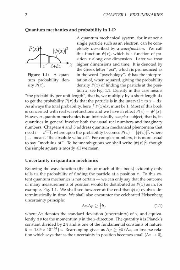
Figure 1.1: A quan-tum probability den-sity P(x).

A quantum mechanical system, for instance asingle particle such as an electron, can be com-pletely described by a wavefunction. We callthis function ψ(x), which is a function of po-sition x along one dimension. Later we treathigher dimensions and time. It is denoted bythe Greek letter “psi”, which is pronounced asin the word “psychology”. ψ has the interpre-tation of, when squared, giving the probabilitydensity P(x) of finding the particle at the posi-tion x; see Fig. 1.1. Density in this case means

“the probability per unit length”, that is, we multiply by a short length dx

to get the probability P(x)dx that the particle is in the interval x to x + dx.As always the total probability, here

∫P(x)dx, must be 1. Most of this book

is concerned with real wavefunctions and we have in effect P(x) = ψ2(x).However quantum mechanics is an intrinsically complex subject, that is, itsquantities in general involve both the usual real numbers and imaginarynumbers. Chapters 4 and 5 address quantum mechanical phenomena thatneed i =

√−1, whereupon the probability becomes P(x) = |ψ(x)|2, where

|. . .| means “the absolute value of”. For complex numbers, it is more usualto say “modulus of”. To be unambiguous we shall write |ψ(x)|2, thoughthe simple square is mostly all we mean.

Uncertainty in quantum mechanics

Knowing the wavefunction (the aim of much of this book) evidently onlytells us the probability of finding the particle at a position x. To this ex-tent quantum mechanics is not certain — we can only say that the outcomeof many measurements of position would be distributed as P(x) as in, forexample, Fig. 1.1. We shall see however at the end that ψ(x) evolves de-terministically in time. We shall also encounter the celebrated Heisenberguncertainty principle:

∆x.∆p ≥ 12 h , (1.1)

where ∆x denotes the standard deviation (uncertainty) of x, and equiva-lently ∆p for the momentum p in the x-direction. The quantity h is Planck’sconstant divided by 2π and is one of the fundamental constants of nature:h = 1.05× 10−34 J s. Rearranging gives us ∆p ≥ 1

2 h/∆x, an inverse rela-tion which says that as the uncertainty in position becomes small (∆x → 0),

1.1. MOVING FROM CLASSICAL TO QUANTUM 3

then the uncertainty in momentum, ∆p, gets very large. Speaking loosely,if we confine a quantum particle in space it moves violently about. We can-not know both spatial and motional information at the same time beyond acertain limit.

There is another important consequence of uncertainty. For wavefunc-tions with small average momentum 〈p〉, ∆p is a rough measure of the mag-nitude of the momentum p of the particle1. Given that p = mv, with m themass and v the speed, and that the kinetic energy is T = 1

2 mv2 = p2/2m,then

T ≥ h2

2m

1(∆x)2 . (1.2)

As we confine a particle, its energy rises. This “kinetic energy of confine-ment”, as it is known, gives rise, for instance, to atomic structure when theconfining agent is electromagnetic attraction and to relativistic particle/anti-particle pair production when the energy scale of T is ≥ 2mc2, that is morethan twice the Einsteinian rest mass energy equivalent.

Measurement and wave–particle duality in Quantum Mechanics

Quantum mechanical particles having a probability P(x) of being found atx, means that the outcomes of many measurements are distributed in thisway. Any given measurement has a definite result that localises the particleto the particular position in question. We say that the wavefunction col-lapses on measurement. Knowing the position exactly removes any knowl-edge we might have had about the momentum, as we have seen above. Inquantum mechanics physical variables appear in conjugate pairs, in fact thecombinations that appear together in the uncertainty principle. Positionand momentum are a basic pair, of which we cannot be simultaneously cer-tain. Another pair we meet is time2 and energy. Measurement of one givesa definite result and renders the other uncertain. Notice that momentum isthe fundamental quantity, not velocity.

It will turn out that the wavefunction ψ will indeed describe waves,and thus also the fundamentally wave-like phenomena such as diffractionand interference that quantum mechanical particles exhibit. For electrons

1Consider for instance a particle where the momentum takes the values +p or −p. So〈p〉 = 0. The mean square of the momentum is clearly p2, and the root mean square, thatis, the standard deviation, ∆p = p simply. If p takes a spread of values, then ∆p is not soprecisely related to any of the individual p values, but it still gives an idea of the typical sizeof the momentum.

2Time is special as it is not a true dynamical variable.


the appropriate “slits” leading to diffraction and then interference are actu-ally the atoms or molecules in a crystal. They have a characteristic spacingmatched to the wavelength of electrons of modest energy. A probabilityP(x) of finding diffracted particles, for instance, on a plane behind a crys-tal is reminiscent of the interference patterns developed by light behind ascreen with slits. However the detection of a particle falling on this planewill localise it to the specific point of detection — particles are not individu-ally smeared out once measured. Thus a wave-like aspect is required to geta P(x) characteristic of interference, and a particle-like result is observed inindividual measurements; this is the celebrated wave–particle duality. InChapter 4 we show pictures of particles landing on a screen, but distributedas if they were waves!

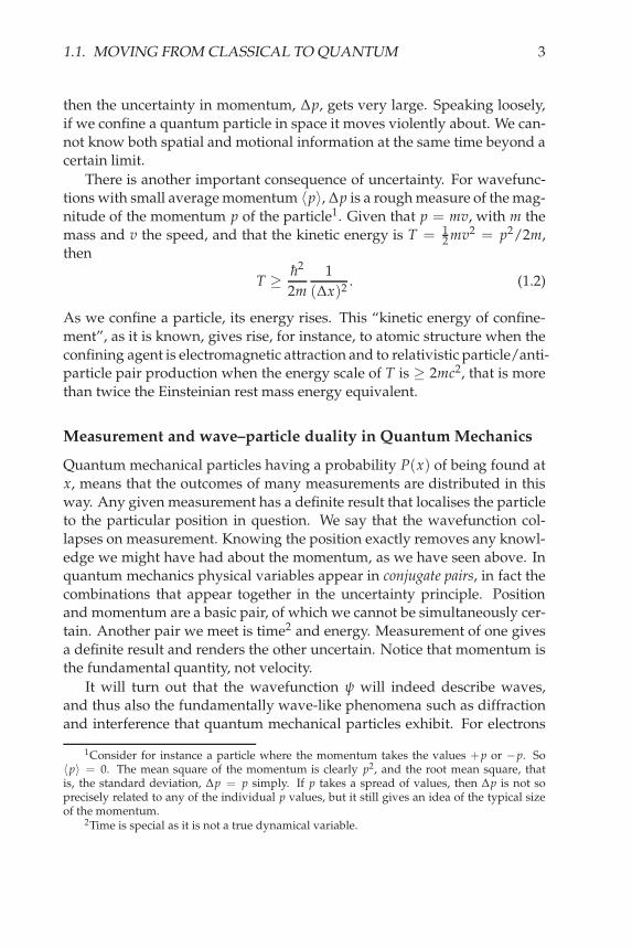
Figure 1.2: G.P. Thomson — Nobel Prize (1937; with Davisson)for diffraction of electrons as quantum mechanical waves, andJ.J. Thomson — Nobel Prize (1906) for work “on conduction of elec-tricity by gases”, middle row, 2nd and 4th from left respectively. Inthis class photo of Cavendish Laboratory research students in 1920there are four other Nobel prize winners to be identified — see thisbook’s web site for answers.

The electron was discovered as a fundamental particle by J.J. Thomsonusing apparatus reminiscent of the cathode ray tube as in an old fashioned


TV. His son, G.P. Thomson, a generation later discovered the electron as awave using diffraction (through celluloid); see Fig. 1.2. Both father and sonseparately received Nobel Prizes in physics for discovering the oppositeof each other! J.J. was Cavendish Professor in Cambridge (the supervisorand predecessor of Rutherford), and was Master of Trinity College, Cam-bridge. G.P. made his Nobel discovery in Aberdeen, did further fundamen-tal work at Imperial College, and was Master of Corpus Christi College inCambridge.

Potentials and forces

Unlike the standard treatments of classical mechanics in terms of forces,quantum mechanics deals more naturally in terms of energies. In particu-lar, the role of a force is replaced by its potential energy. Forces betweenparticles, or for instance those exerted by a spring, do work when the par-ticles move or a spring changes length. The energy stored in the field orspring is potential energy V(x), a function of separation, extension, etc. x.Movement of the point of application of the force, f , against its directionby −dx gives an increase in the stored energy dV = − f dx (“force timesdistance”), that is, force is given by f = −dV/dx. Note the − sign. Onespeaks simply of a potential V(x) which, if it changes with position, givesrise to forces.

Famous examples of potentials include

V(x) = +Q1Q2

4πǫ0x(Coulomb/electric)

= −Gm1m2

x(gravitation)

= + 12 qx2, (harmonic)

where the first gives the Coulomb repulsive/attractive force between twocharges Q1 and Q2 depending on their relative signs, and the second givesthe gravitational attractive force between two masses m1 and m2, the chargesand masses being a distance x apart. The third potential gives the retractiveforce−qx when a spring is stretched by x away from its natural length. Theconstants that determine the scale of the potential, ǫ0, G and q are the per-mittivity of free space, the gravitational constant and the spring constant,respectively. We shall explore quantum motion and energies in potentialsof various shapes.

It is important to think about and solve the problems posed in the text.Mostly they will have at least some hint to their solution. The problems


a

EV0

a/2a/2

Figure 1.3: A finite square well of depth V0.

in part illustrate the principles under discussion. But physics and mathsare subjects only really understood when one can “do”. Problems are theonly route to this understanding, and also give fluency in the core (mathe-matical) skills of physics. So repeat for yourself even the problems wherecomplete or partial solutions have been given.

Exercise 1.1: Derive from the electric, gravitational and harmonic potentialstheir force laws. Explain the sign of the forces — is it what you expect? Takecare over the definition of the zero of potential. Does the position where thepotential is zero matter?

Subsequent problems explore the shift from using forces to potentialsin analysing a problem. For instance, to calculate the change in speed ofa particle, you might have considered a force-displacement curve. This isa diagram which tells you what forces are acting as a function of the po-sition of the particle. In fact, one would need to know the area under thecurve, which amounts to the change of energy of the particle (from poten-tial energy to kinetic energy or vice versa). We can avoid having to knowsuch detail by simply using the potential energy graph. These ideas are bestillustrated by the following examples.

Exercise 1.2: Consider a particle of mass m passing a potential well of widtha, as shown in Fig. 1.3. The particle has total energy E > V0, the depth ofthe well. Calculate the time taken by the particle to traverse the figure.

Solution: First, we note that the well is a schematic of the energies and weare asked to use energies directly rather than forces. Secondly, the nature ofthe forces is irrelevant — this is the advantage of an energy approach. Thediagram is not describing a dip in a physical landscape.


In the regions outside the well, the kinetic energy is the difference be-tween the total energy E and the potential energy V0

12

mv2 = E−V0. (1.3)

So the speed is given by v =√

2(E−V0)m . Inside the well, all the energy is

entirely kinetic and so the speed is v′ =√

2Em . Making use of the definition

of speed, we find the total time

t =

√

ma2

2

(1√E+

1√E−V0

)

. (1.4)

Exercise 1.3: A particle of mass m slides down, under gravity, a smoothramp which is inclined at angle θ to the horizontal. At the bottom, it isjoined smoothly to a similar ramp rising at the same angle θ to the horizon-tal to form a V-shaped surface. If the particle slides smoothly around thejoin, determine the period of oscillation, T, in terms of the initial horizontaldisplacement x0 from the centre join. Note the shape of the potential well.

Hint: We see that the potential well appears as a sloping line similar to theone along which the particle is constrained to move. It is only this linearslope at angle θ to the horizontal, that happens to resemble the potentialenergy graph of the same shape, which misleads us into thinking that wecan see the potential energy. The potential energy is a concept, representedpictorially by a graph and the shape of the graph happens, in some cases,to resemble the mechanical system.

The distinction between the actual landscape (flat) and the potential isclear in the case of a quadratic potential. See Fig. 3.4 on page 55.

Exercise 1.4: A particle moves in a potential V(x) = 12 qx2. If it has total

energy E = E0 give an expression for its velocity as a function of positionv(x). What is the amplitude of its motion?

Exercise 1.5: The potential energy of a particle of mass m as a function of itsposition along the x axis is as shown in Figure 1.4.(a) Sketch a graph of the force versus position in the x direction which acts


E = V1 3 0

E = V2 5 0

2V0

4V0

a

a/2

Figure 1.4: A stepped rectangular potential well

on a particle moving in this potential well with its vertical steps. Why isthis potential unphysical?(b) Sketch a more realistic force versus position curve for a particle in thispotential well. For a particle moving from x = 0 to x = 3a

2 , which waydoes the force act on the particle? If the particle was moving in the oppositedirection, which way would the force be acting on the particle?

Hint: Take care over the physical meaning of the potential energy. It canlook misleadingly like the physical picture of a particle sliding off a highshelf, down a very steep slope and then sliding along the floor, reflectingoff the left hand wall and then back up the slope. This is too literal an in-terpretation since, for example, the potential change might be due to anelectrostatic effect rather than a gravitational one, and the time spent mov-ing up or down the slope is due to artificially putting in an extra verticaldimension in a problem which is about motion in only one dimension. Anexample of where there is literally motion vertically as well as horizontally,is that of a frictionless bead threaded on a parabolic wire. The motion isnot the same as in the one-dimensional simple harmonic motion of Ex. 1.4.Although the potential energy is expressible in the form 1

2 qx2 due to theconstraint of the wire, the kinetic energy involves both the x and y vari-ables.

Exercise 1.6: Consider again the particle in Ex. 1.5. If it has a total mechanicalenergy E equal to 3V0, calculate the period for a complete oscillation.

Quantum mechanics in the world around us

Quantum effects are mostly manifested on a length scale much smaller thanwe can observe with light and hence are not directly part of our everyday

1.2. MATHEMATICAL PRELIMINARIES 9

world. Indeed we shall see that quantum mechanics takes us far from ourcommon experience. A particle can be in two places at the same time — itmust pass through at least two slits for interference to occur — and we shallsee the need to think of them as having a wave–particle duality of character.But our world is dominated by the macroscopic effects of quanta. The con-ductivity of metals and semiconductors is entirely dominated by quantumeffects and without them there would be no semiconductor age with com-puters, consumer electronics, digital cameras, telecommunications, modernmedical equipment, or lasers with which to read digital discs. Atomic andmolecular physics, chemistry, superconductivity and superfluidity, electrontransfer in biology are all dominated by quantum mechanics. It is withquantum mechanical waves, in an electron microscope, that we first sawthe atomic world. The ability of quantum particles to tunnel through classi-cally forbidden regions is exploited in the scanning tunnelling microscopeto see individual atoms.

We shall explore such fundamental effects. For instance, we shall seehow quantum particles explore classically forbidden regions where theyhave negative kinetic energy and should really not venture. We shall evenat the end quantise a model of electromagnetic standing waves and see howphotons and phonons arise. However fundamental the phenomena we ex-amine, and those that more advanced courses deal with, these effects haveall had a revolutionary influence in the last century through their applica-tions to technology, and have fashioned the world in which we live.

1.2 Mathematical preliminaries for quantum mechanics

Probability, trigonometric and exponential functions, calculus, differential equa-tions, plotting functions and qualitative solutions to transcendental equations

Mathematics suffuses all of physics. Indeed some of the most importantmathematics was developed to describe physical problems: for exampleNewton’s description of gravitational attraction and motion required hisinvention of calculus. If you are good at maths, and especially if you en-joy using it (for instance in mechanics), then higher physics is probably foryou even if this is not yet clear to you from school physics. This book de-pends on maths largely established by the end of the penultimate year atschool. We simply sketch what you have learned more thoroughly already,but might not yet have practised much or used in real problems. So we as-sume exposure to trigonometric and exponential functions, and to differen-tiation and integration in calculus. We later introduce some more elaborate


forms of what you know already — for instance the extension of algebra tothe imaginary number i and its use in the exponential function, and differ-entiation with respect to one variable while keeping another independentvariables constant (partial differentiation).

Practice is the only path to becoming good at maths and to eventuallyfinding its execution and applications simple. The examples given through-out these notes are designed to illustrate the physics, but more importantlythey will give you fluency and confidence in maths so that it is never anissue in your understanding the physics.

Probability

Wavefunctions generate probabilities, for instance that of finding a particlein a particular position. We shall use probabilities throughout these notes,taking averages, variances etc. Familiar averages over a discrete set of out-comes i are written, for instance:

〈x〉 = ∑i

xi pi and 〈 f (x)〉 = ∑i

f (xi)pi . (1.5)

Here 〈〉 around a quantity means its average over the probabilities pi. Thisis called the expectation value of the quantity. When outcomes are continu-ously distributed, we replace the pi by a probability density (probability perunit length) P(x) which gives a probability P(x)dx that an outcome falls inthe interval x to x + dx. Just as the discrete probabilities must add up to 1,so do the continuous probabilities:

∑i

pi = 1→∫

P(x)dx = 1 . (1.6)

Such probabilities are said to be normalised. If the probability is not yet nor-malised, we can still use it but we must divide our averages by

∫P(x)dx,

which is in effect just performing the normalisation. You will see that insome problems it pays to delay this normalisation process in the hope thatit eventually cancels between numerator and denominator. Thus averages(1.5) become

〈x〉 =∫

xP(x)dx and 〈 f (x)〉 =∫

f (x)P(x)dx . (1.7)


Exercise 1.7: The variance σ2 in the values of x is the average of the squareof the deviations of x from its mean, that is,

σ2 = 〈(x− 〈x〉)2〉 .

Prove the above agrees with the standard result σ2 = 〈x2〉 − 〈x〉2 for bothdiscrete and continuous x.

Essential functions for quantum mechanics

We shall see that a particle in a constant potential V(x) = V0, say, is rep-resented by a wavefunction ψ ∝ sin(kx), where ∝ means “proportionalto” (that is, we have left off the constant of proportionality between ψ andsin(kx)). The argument of the sine function, the combination kx, can bethought of as an angle, say θ = kx. It must be dimensionless, as the argu-ment for all functions must be — this is a good physics check of algebra!Hence k must have the dimensions of 1/length and we shall return to itsmeaning in Chapter 2.3. ψ could equally be represented by cos(kx) with achange of phase. We shall constantly use properties of trigonometric func-tions, among the simplest being:

sin2 θ = 1− cos2 θ (1.8)

cos(2θ) = 2 cos2 θ − 1 = 1− 2 sin2 θ (1.9)

sin(2θ) = 2 sin θ cos θ (1.10)

tan θ = sin θ/ cos θ (1.11)

sin θ + sin φ = 2 sin(

θ + φ

2

)

cos(

θ − φ

2

)

(1.12)

The double angle relations (1.9) and (1.10) are sometimes used in integralsin rearranged form, e.g. sin2 θ = 1

2 (1 − cos(2θ)). The addition formula(1.12) is used when adding waves together.

In quantum mechanics it is possible to have negative kinetic energy,something that is classically forbidden since clearly our familiar form isT = p2/2m ≥ 0. If while T < 0 the potential is also constant, V(x) = V0,then the wavefunction will have the form ψ ∝ e−kx or ∝ ekx, depending onwhether x is increasing or decreasing respectively. The function ex is the ex-ponential. We shall find sin, cos and exp as functions whose oscillations inwells, and decay away from wells, describe localised quantum mechanicalparticles.


The Gaussian function e−x2/2σ2has a very special place in the whole of

physics. The form given is the standard form complete with the factor of2 and its characteristic width σ for reasons made clear in Ex. 1.14. It isthe wavefunction for the quantum simple harmonic oscillator in its groundstate and is also the wavefunction with the minimal uncertainty. We returnto it at the end of Chapter 3.

Exercise 1.8: Plot e−x2/2σ2for a range of positive and negative x. Label im-

portant points on the x axis (including where the function is 1/e) and they axis. Pay special attention to x = 0, including slope and curvature there.What is the effect on the graph of varying σ?

A little calculus — differentiation

The first derivative of the function f (x), denoted by d f /dx, is the slope off . Figure 1.5 shows the tangent to the curve f (x) and, in a triangle, howthe limit as δx → 0 of the ratio of the infinitesimal rise δ f to the incre-ment δx along the x axis gives tan θ and hence the slope of f (x) at a point.Vitally important is the second derivative d2 f /dx2 since this leads to thequantum mechanical kinetic energy, T. It is the rate of change of the slope.Figure 1.5 shows regions of increasing/decreasing slopes and hence posi-tive/negative second derivatives. The second derivative is in effect the rate

Figure 1.5: The gradient d f /dx =tan θ of the function f (x). The sec-ond derivative d2 f /dx2 is positiveat the minimum where the slope isincreasing with x. The curvature,1/R, derives from the circular arc,of radius R, fitted to f (x) at x. d d >0

2f x/

2d d <0

2f x/

2

δf

δx

θf x( )

R

at which the curve deviates from its local tangent. We shall also loosely re-fer to it as the “curvature”. Figure 1.5 shows an arc of a circle of radius Rfitted to a minimal point, a point of zero slope where the second derivativeis exactly d2 f /dx2 = 1/R. Away from minima or maxima, but for not toogreat a slope, the curvature is approximately the second derivative 3.

3A precise definition for the curvature is 1/R = d2 f /dx2/(1+ (d f /dx)2)3/2 which takesaccount of an increment δx not being the same as an increment of length along the curve.


We require derivatives of the most common functions encountered inquantum mechanics:

ddx

sin(kx) = k cos(kx) (1.13)

ddx

cos(kx) = −k sin(kx) (1.14)

ddx

ekx = kekx. (1.15)

The latter is a definition of the exponential function — the function that is itsown derivative. To see this relation, we make the substitution u = kx intoEq. (1.15). The derivatives become d

dx = dudx

ddu = k d

du and so we find thatd

du eu = eu. Another common function in physics is the inverse function tothe exponential — the natural logarithm. Consider the curve y = ex. Theinverse function is

x = ey. (1.16)

To see this we sketch both functions on the same axes, Fig. 1.6. We write the

1

1

y x( ) (a)

(b)

x

Figure 1.6: Plots of (a) y(x) = ex and (b) y(x) = ln(x). They arereflections of each other in the line y = x and thus one can think of(b) as x = ey.

solution to Eq. (1.16) as y = ln x. The derivative may be found by making

use of the result for derivatives of inverse functions, viz. dydx = 1/(dx

dy ). Sincedxdy = ey = x we have

ddx

ln x =1x

. (1.17)


Exercise 1.9: Plot sin(kx), cos(kx), e±kx and ln(kx) for a range of positive andnegative x. Label important points (e.g. intersections with axes, maximaand minima) on the x and y axes. What happens to these points and thegraph if you change k? Revise elementary properties of the exponentialand logarithmic functions. What are (ex)2, ex/ey, a ln x and ln x + ln y?

At http://www.periphyseos.org is a dynamic applet which shows theeffect of changing k.

We often need to differentiate the product of two functions:

ddx

(g(x).h(x)) =dg(x)

dx.h(x) + g(x).

dh(x)

dx, (1.18)

which is the product rule.Sometimes we shall differentiate a function of a function for which one

requires the chain rule.

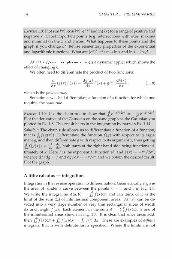
Exercise 1.10: Use the chain rule to show that ddx e−x2/2σ2

= − xσ2 e−x2/2σ2

.Plot the derivative of the Gaussian on the same graph as the Gaussian youplotted in Ex. 1.8. This result helps in the integration by parts in Ex. 1.14.

Solution: The chain rule allows us to differentiate a function of a function,that is d

dx f (g(x)). Differentiate the function f (g) with respect to its argu-ment g, and then differentiate g with respect to its argument x, thus gettingd

dx f (g(x)) = d fdg ·

dgdx , both parts of the right hand side being functions ul-

timately of x. Here f is the exponential function eg, and g(x) = −x2/2σ2,whence d f /dg = f and dg/dx = −x/σ2 and we obtain the desired result.Plot the graph.

A little calculus — integration

Integration is the reverse operation to differentiation. Geometrically, it givesthe area, A, under a curve between the points x = a and b in Fig. 1.7.

We write the integral as A(a, b) =∫ b

a f (x)dx and can think of it as thelimit of the sum (Σ) of infinitesimal component areas. A(a, b) can be di-vided into a very large number of very thin rectangular slices of widthdx and height f (x). Each element in the sum A = ∑

ba f (x)dx is one of

the infinitesimal areas shown in Fig. 1.7. It is clear that since areas add,

then∫ b

a f (x)dx +∫ c

b f (x)dx =∫ c

a f (x)dx. These are examples of definite

integrals, that is with definite limits specified. Where the limits are not


f x( )

xa b c dx

A a b( , )

area=f x x( ).d Figure 1.7: Integration gives the

area under a curve of the func-tion. Integrals can be added, thusA(a, b) + A(b, c) = A(a, c).

given these integrals are termed indefinite. Commonly, there is no dis-tinction made between independent and dummy variables. For example,∫

exdx = ex has x as the same variable for both sides. We shall not abusethis notation. For instance,

∫ xsin(kz)dz = −1

kcos(kx) + c1 (1.19)

∫ x

cos(kz)dz =1k

sin(kx) + c2 (1.20)∫ x

ekzdz =1k

ekx + c3. (1.21)

Note that an arbitrary constant (c1, c2, c3 in the above) then arises in each in-tegration. It can be thought of related to the starting point of the integrationwhich has been left indefinite. To reconcile the absent lower limit to the ap-pearance of an arbitrary constant, consider as an example

∫ xa ezdz = ex− ea.

If a is an arbitrary constant, then so is the constant ea. Upon differentiationthese constants are removed. The variable of integration, z, is a dummyvariable — any symbol can be used. This is identical to the dummy in-dex used in discrete sums. For instance, the sum ∑i xi is the same as ∑j xj.The only difference is that z in the former example is a continuous variablewhereas i and j are discrete.

Exercise 1.11: Confirm by differentiation of the right hand sides of Eqs. (1.19–1.21) that, in these cases at least, differentiation is indeed the reverse processfrom integration; that is, d

dx

∫ xf (z)dz = f (x) in the above examples.

The result is generally true; take I(x + dx) =∫ x+dx

f (z)dz and sub-tract from it I(x) =

∫ xf (z)dz. Use the ideas in Fig. 1.7 of adding or sub-

tracting integrals to construct dIdx = lim

dx→0

I(x+dx)−I(x)dx . The numerator is

clearly A(x, x +dx) which, from the definition of integration, is in this limitf (x).dx. Putting this result in and cancelling the dx factors top and bottom,one obtains dI

dx = f (x).


Integration by parts

Integration by parts is frequently useful in quantum mechanics. It canbe thought of as the reverse of differentiation of a product. IntegratingEq. (1.18) gives

∫ b

a

ddx

[g(x).h(x)]dx =∫ b

a

dg(x)

dx.h(x)dx +

∫ b

ag(x).

dh(x)

dxdx. (1.22)

Rearranging we find that

∫ b

ag(x).

dh(x)

dxdx = [g(x).h(x)]ba −

∫ b

a

dg(x)

dx.h(x)dx . (1.23)

Notice that h on the right hand side can be regarded as the indefinite inte-gral of the dh/dx factor on the left hand side, that is h(x) =

∫ x dhdz dz. For

clarity rewriting g as u(x) and dh/dx as v(x), one can rewrite in a formeasier to remember and apply:

b∫

a

u(x).v(x)dx =

[

u(x).(∫ x

v(z)dz

)]b

a

−b∫

a

(du

dx

)

.(∫ x

v(z)dz

)

dx .

(1.24)Be fluent with the use of the result. Our experience shows that it is best toremember it for use directly along the lines of

“to integrate a product (uv), integrate one part (v) and evaluatethis integral times the other function between the given limits,that is giving the first term on the right. Take away the inte-gral of [(the integral already done)×(the derivative of the otherfactor)], giving the second term on the right.”

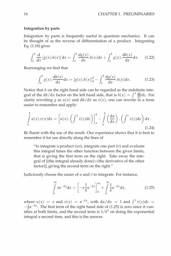
Judiciously choose the easier of u and v to integrate. For instance,

∞∫

0

xe−kxdx =

[

−x1k

e−kx

]∞

0+

∞∫

0

1k

e−kxdx, (1.25)

where u(x) = x and v(x) = e−kx, with du/dx = 1 and∫ x

v(z)dz =− 1

k e−kx. The first term of the right hand side of (1.25) is zero since it van-ishes at both limits, and the second term is 1/k2 on doing the exponentialintegral a second time, and this is the answer.


Exercise 1.12: Integrate∫ ∞

0 xne−xdx once by parts. The result suggests rep-etition until the final result. What well-known function results?

Exercise 1.13: Integrate∫ π

20 x2 sin x dx and

∫ π2

0 x2 cos x dx.

The split into u and v can require delicacy! For example, the integral∫ ∞

−∞x2e−x2/2σ2

dx can be written as∫

u.vdx =∫(−σ2x).

(

− xσ2 e−x2/2σ2

)

dx.

Identifying v(x) as the second factor, the integral∫ x

v(z)dz = e−x2/2σ2is

easy; see in Ex. 1.10 the differentiation of this answer back to the startingpoint, and du/dx = −σ2 is also easy. The integral has been reduced toanother one which does not have a simple answer, but that itself is not nec-essarily a difficulty — a problem delayed is sometimes a problem solved!

Exercise 1.14: If P(x) ∝ e−x2/2σ2, what is the average 〈x2〉?

This Gaussian result is found throughout physics and is worth remem-bering:

“From a Gaussian probability written in its standard form P(x) ∝

e−x2/2σ2, one reads off the mean square value of x as being σ2,

that is, the number appearing in the denominator of the expo-nent, taking care to re-arrange slightly if the required factor oftwo is not directly apparent.”

What would be the mean square value of x be if the probability were P(x) ∝

e−2x2/b2? Answer: 〈x2〉 = b2/4.

The reader eager to get on to quantum mechanics could skip the nextproblems, quickly revise differential equations, and jump to Chapter 2. Itwill be obvious to you when it is to your advantage to return to this exer-cise.

Exercise 1.15: Evaluate N =∫ L

0 sin2(πxL )dx and 1

N

∫ L0 x2 sin2(πx

L )dx.

Hint: Use a double angle result and integration by parts. N = L/2, a re-sult that is rather general for the integration of squares of sine and cosinethrough intervals that defined as being between various of their nodes. Af-ter studying quantum wells you might like to return to the choice π/L for

the coefficient of x in the argument of sine. The second result is L2(

13 − 1

2π2

)

.


Given your result for N, then 1N sin2(πx/L) would be an acceptable proba-

bility P(x). What is 〈x〉? What is the variance of x?

Exercise 1.16: Integrate the functions ln x, ln xx2 and ln(sin x)

cos2 x.

Differential equations

Most of physics involves differential equations and they certainly underpinquantum mechanics. Such equations involve the derivatives of functions aswell or instead of the usual familiar algebraic operators in simple equationssuch as powers. The first differential equations we meet are those of freemotion, or motion with constant acceleration, such as free fall with g. Thusforce = mass times acceleration is the differential equation mdv/dt = mg.It is easily integrated once with respect to time t: the right hand side isconstant in time and gives mgt. The left hand side has the derivative nul-lified by integration to give mv + constant. Cancelling the masses, givesv = v0 + gt. We have taken the initial speed (at t = 0) as v0, that is, wehave fixed the constant of integration by using an initial condition. Moregenerally, these are termed boundary conditions. Rewriting the answer asdz/dt = v0 + gt, where z is the distance fallen down, we can integrate bothsides again to yield z = v0t + 1

2 gt2, where we have taken the next constantof integration, the position z0 at t = 0, to be zero. This familiar result ofkinematics is actually the result of solving a differential equation with asecond order derivative since we could have written our starting equationas d2z/dt2 = g.

Exercise 1.17: For the mass under free fall described above, sketch on thesame axes the acceleration dv

dt , velocity v and displacement z as a functionof time.

Simple harmonic motion

Ubiquitous throughout physics is simple harmonic motion (SHM) or thesimple harmonic oscillator (SHO) which for instance in dynamics resultswhen a particle of mass m is acted on by a spring exerting a force−qz wherenow z denotes the particle’s displacement from the origin. The correspond-ing potential giving rise to the force is harmonic — see the discussion ofpotentials on page 5. The − sign indicates that the force is restoring, that is,


opposite in direction to the displacement, and q is Hooke’s constant. New-ton’s second law is f = ma with the acceleration a = dv

dt being the timederivative of the velocity, that is, of v = dz

dt . Using the Hookean force, oneobtains the equation of motion

md2z

dt2 = −qz ord2z

dt2 = −ω2z , (1.26)

where the angular frequency, ω, will be discussed below and is clearlyω =

√q/m. This equation describes oscillations of the particle here, but

in a general form also those of an electric field in electromagnetic radia-tion, or the quantum fields in quantum electrodynamics. Thus differentialequations differ from the usual kinds of algebraic equations since they in-volve derivatives of the function. The highest derivative in (1.26) is a sec-ond derivative and so (1.26) is called a second order (ordinary) differentialequation. The “ordinary” means there is only one independent variable,t here. We shall later meet cases of more than one independent variablewhich give rise to “partial” differential equations.

An honourable and perfectly legitimate method of solving differentialequations is to guess a solution and try it out. Guesses can often be verywell informed and hence this is not entirely magic!

Exercise 1.18: Inspect Eqs. (1.13–1.15) and differentiate each side again. Con-firm that for f = sin(kx) and cos(kx), and separately for f = e±kx, one hasrespectively the similar results:

d2 f

dx2 = −k2 f andd2 f

dx2 = k2 f . (1.27)

In a mysterious way ekx is like sin(kx) or cos(kx), but with k2 replacedby −k2. This turns out to be true, but there is the little matter of a squarednumber becoming negative! (52 = 25 and (−5)2 = 25 too; how would oneget a result of −25?) We treat imaginary and complex numbers in Chap-ter 4.1 which could also be read now if desired.

Considering time t rather than x as the independent variable, one canconfirm that two solutions for SHM (Eq. (1.26)) are

z(t) = zs sin(ωt) , z(t) = zc cos(ωt). (1.28)

Since sine and cosine repeat when ωt = 2π, that is, after a period t = T =2π/ω, then rearrangement shows that ω = 2π/T ≡ 2πν — the angular


frequency where ν = 1/T is the usual frequency. The amplitudes zs and zc

of oscillation are arbitrary and indeed the general solution would be z(t) =zs sin(ωt) + zc cos(ωt), which is an arbitrary combination of the oscillatorycomponents differing in phase by π/2 or 90 degrees.

We have seen in the second order differential equation (1.26), a constantis introduced every time we integrate. Two integrations and thus two con-stants are required to get a general solution. How do we fix these constants?“Boundary conditions”, in this case two, and in general as many as the or-der of the equation, are required to fully solve differential equations. Herefor instance, at t = 0 we have z(t = 0) = 0 and dz/dt = v0 (the particleis initially at the origin with velocity v0). The first condition demands thatzc = 0 (recall what sin(0) and cos(0) are). The second condition gives

v0 =dz

dt

∣∣∣∣t=0

= ωzs cos(ωt)|t=0 = ωzs ,

that is zs = v0/ω. See also the simple example above of integrating thedifferential equation of free fall. Note that the period (T = 2π/ω) is in-dependent of the amplitude: only the ratio between the inertia factor (themass) and the elasticity factor (the spring constant) matters. This is gener-ally not true. See Ex. 1.3 where the period increases with amplitude andEx. 1.33 for more exotic behaviour. Consult Sect. 3.2 for further discussionof classical SHM.

x

mq

Figure 1.8: A mass on a light spring.

Exercise 1.19: A mass m, attached to a light spring of constant q, slides on ahorizontal surface of negligible friction, as shown in Figure 1.8. The mass isdisplaced through a distance x0 from the equilibrium position and released.Write down Newton’s 2nd law as applied to the displaced mass.

A clock is started at some later time and the dependence of the displace-ment on time is given by x(t) = x0 sin(ω t + φ). Act on the time dependent

displacement x(t) with the operator d2

dt2 . You will see that the same functionis obtained up to a multiplicative constant. Obtain the constant and relate


it to the result of Newton’s 2nd Law.

Sketch a graph of the system’s potential energy versus displacement.

Exponentially decaying motion

If friction dominates, that is, if there is no or insufficient restoring force, wehave instead exponential instead of sinusoidal motion.

Exercise 1.20: A block sliding on a surface suffers a retarding force propor-tional to its velocity, f = −µv, where µ is a constant. Show that dv/dt =−(µ/m)v and solve the equation subject to v(t = 0) = v0. What is the dis-placement as a function of time? Sketch the block’s displacement, velocityand acceleration as a function of time on the same axes.

Solution: Applying Newton II gives m dvdt = −µv. This is a first order sepa-

rable differential equation. The solution can be found by either comparisonwith radioactive decay or by separating variables. Performing the latteryields dv

v = − µm dt. Integrating and inserting the boundary condition gives

∫ v

v0

dv

v= − µ

m

∫ t

0dt (1.29)

ln(

v

v0

)

= − µ

mt (1.30)

v = v0e−µm t. (1.31)

Note that there is only one boundary condition since it is a first order dif-ferential equation. Check that this is indeed a solution to the differentialequation (and the initial condition) by direct substitution. A further inte-

gration produces the displacement mv0µ

(

1− e−µm t)

at time t.

Exercise 1.21: A model for a parachutist’s downward speed v(t) at time t infree fall after jumping out is given by

mdv

dt= mg− kv. (1.32)

Explain the physical origin of each of the terms. Solve the differential equa-tion (1.32) given his initial speed is zero when he jumps out. What is histerminal velocity?


We return to very general and important aspects of differential equa-tions in Sect. 2.3 on Sturm–Liouville theory.

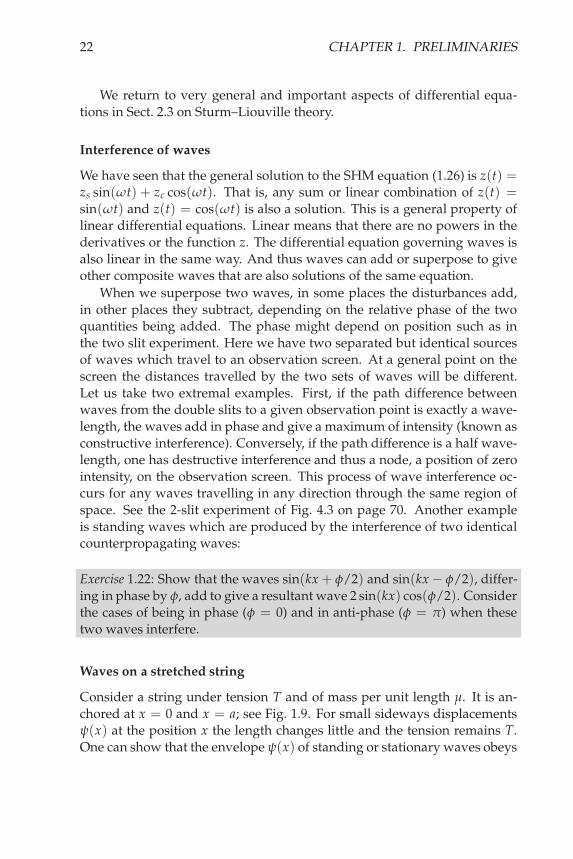
Interference of waves

We have seen that the general solution to the SHM equation (1.26) is z(t) =zs sin(ωt) + zc cos(ωt). That is, any sum or linear combination of z(t) =sin(ωt) and z(t) = cos(ωt) is also a solution. This is a general property oflinear differential equations. Linear means that there are no powers in thederivatives or the function z. The differential equation governing waves isalso linear in the same way. And thus waves can add or superpose to giveother composite waves that are also solutions of the same equation.

When we superpose two waves, in some places the disturbances add,in other places they subtract, depending on the relative phase of the twoquantities being added. The phase might depend on position such as inthe two slit experiment. Here we have two separated but identical sourcesof waves which travel to an observation screen. At a general point on thescreen the distances travelled by the two sets of waves will be different.Let us take two extremal examples. First, if the path difference betweenwaves from the double slits to a given observation point is exactly a wave-length, the waves add in phase and give a maximum of intensity (known asconstructive interference). Conversely, if the path difference is a half wave-length, one has destructive interference and thus a node, a position of zerointensity, on the observation screen. This process of wave interference oc-curs for any waves travelling in any direction through the same region ofspace. See the 2-slit experiment of Fig. 4.3 on page 70. Another exampleis standing waves which are produced by the interference of two identicalcounterpropagating waves:

Exercise 1.22: Show that the waves sin(kx + φ/2) and sin(kx− φ/2), differ-ing in phase by φ, add to give a resultant wave 2 sin(kx) cos(φ/2). Considerthe cases of being in phase (φ = 0) and in anti-phase (φ = π) when thesetwo waves interfere.

Waves on a stretched string

Consider a string under tension T and of mass per unit length µ. It is an-chored at x = 0 and x = a; see Fig. 1.9. For small sideways displacementsψ(x) at the position x the length changes little and the tension remains T.One can show that the envelope ψ(x) of standing or stationary waves obeys


Figure 1.9: A snapshot of standing waveson a stretched string at a particular time.For snapshots of the string at other times,see Fig. 5.6. The transverse displacement isψ(x).

the equation

d2ψ

dx2 = − µ

Tω2ψ. (1.33)

See Sect. 5.3 for a derivation of the full motion, of which this is one limit.For standing sound waves in a tube, ψ(x) would be the pressure that varieswith position x along the tube. The wave speed is c =

√T/µ and ω = 2πν

connects the angular and conventional frequencies, ω and ν. Thus in theabove equation

ω

c=

2πν

c=

2π

λ= k, (1.34)

where these rearrangements employ νλ = c with λ the wavelength. Thefinal definition k = 2π/λ introduces the wavevector that is so ubiquitous inquantum mechanics and optics. Thus the standing wave equation becomes

d2ψ

dx2 = −k2ψ, (1.35)

which is the form of Eq. (1.27). Its solutions are sin(kx) and cos(kx). Fig-ure 1.9 shows that since ψ(0) = 0 we have to discard the cos(kx) solutions,since they are non-zero at x = 0, in favour of sin(kx) solutions that nat-urally vanish at x = 0. Equally in Fig. 1.9, to ensure ψ(x = a) = 0, it isnecessary for an integer number of half wavelengths to be fitted betweenx = 0 and x = a. So

n · λ

2= a ⇒ λ =

2a

n

whence

k =2π

λ=

nπ

a. (1.36)

Only discrete choices of λ, or equivalently k, corresponding to integer n arepermitted. Only certain waves are possible. In fitting waves into this in-terval with its boundary conditions, we have our first encounter with whatwe later see is quantisation!


Qualitative understanding of functions

We shall meet equations we cannot solve exactly. For instance, they can in-volve transcendental functions such as trigonometric and exponential func-tions. However, a deep understanding of the behaviour of quantum sys-tems emerges from plotting the functions, as well as from using calculusand a knowledge of their asymptotes and zeros. For instance Fig. 1.10shows the two functions y =

√x and y = tan(x2). Explain the behaviour

x

f x( )

2

2

−2

−2

−1

−1

1

1

Figure 1.10: A plot of the functions√

x and tan(x2).

of each function at important points such as the origin and at nodes (zeros)of the somewhat unusual tangent function. Why at one node is the slopezero, and why is it finite at others? Where are the nodes in general? Wherethe two functions cross are the solutions of the equation tan(x2) =

√x.

Exercise 1.23: Plot the functions y =√

x0 − x and tan(√

x) on the samegraph for positive x, taking the former function up to x0 (a constant). Iden-tify the zeros and give their values and the behaviour of the functionsaround these zeros, in particular their slopes there. How many solutionsdoes the equation tan(

√x) =

√x0 − x possess. What about the equation

tan(√

x) = −√x0 − x? Similar analysis will be important for quantumwells of finite depth; see Sect. 3.1.

Hint: It might be helpful to differentiate or use the approximation thattan x ≈ x for small x.

We later solve a slightly more complicated version of this problem tofind the characteristic states of a quantum particle found in a finite squarewell; see Eq. (3.8).

A little calculus is sometimes helpful in analysing equations. Anothertranscendental equation is ex = kx; see Fig. 1.11.


x

f x( )

2

3

5

7

1

1

Figure 1.11: Plots of ex, and of kx for various values of k.

Exercise 1.24: For what values of k do there exist solutions of the equationex = kx? What is the solution at the k, say kc, where solutions first appear?

Hint: Consider the case where the line first touches the exponential. Whattwo conditions are required there? Solve them simultaneously.

Exercise 1.25: Consider the equation ex = 12 ax2, for a > 0. For what ranges

of a are there 1, 2, or 3 solutions to this equation?

It is very helpful to know the power series expansions of functions forsmall values of their arguments, and how in general to expand functionsabout an arbitrary point in their range. To get a first approximation recallthat the derivative is the limiting ratio as δx → 0

dy

dx≃ δy

δx≃ y(x0 + δx)− y(x0)

δx. (1.37)

Rearranging we find that

y(x0 + δx) ≃ y(x0) + δx · dy

dx

∣∣∣∣x0

, (1.38)

so we have some knowledge of y at another point (x0 + δx) if we knowy(x0) and the first derivative at x0. We shall use a rearrangement of the firstof Eq. (1.38) to get the difference of the values of a function evaluated at two

different points: y(x0 + δx)− y(x0) ≃ δx · dydx .

Repeated application of this procedure gives us better knowledge fur-ther away, at the expense of needing higher derivatives. So we may write


in terms of derivatives evaluated at x = x0, the Taylor expansion

y(x0 + δx) = y(x0) + δxdy

dx+

(δx)2

2!d2y

dx2 +(δx)3

3!d3y

dx3 + . . . (1.39)

For instance, some familiar functions expanded about x0 = 0 while callingδx simply x:

sin(x) = x− x3

3!+

x5

5!− . . . (1.40)

cos(x) = 1− x2

2!+

x4

4!+ . . . (1.41)

ex = 1 + x +x2

2!+

x3

3!+ . . . (1.42)

11− x

= 1 + x + x2 + . . . (1.43)

tan x = x +x3

3+

2x5

15+ . . . . (1.44)

Exercise 1.26: Confirm the expansions (1 + x)n = 1 + nx + n(n−1)2! x2 + . . .

and tan(x) = x + x3/3 + . . . .

Hint: Recall that tan(x) = sin(x)/ cos(x) and expand the denominator upinto the numerator using (1.43) with a more complicated “x”.

Exercise 1.27: For each of the functions in Eqns. (1.40–1.42), sketch the func-tion, the separate terms in the approximation, and finally the sum of thoseterms on the same diagram.

Hint: Note how each successive term builds up to form a better approxima-tion to the true function. There is an applet on our website which showsthis dynamically.

Vectors

In Sect. 1.2 and Ex. 1.17, we analysed the downwards motion of a fallingparticle. Suppose we had fired the mass horizontally with speed v0 at timet = 0. What is the subsequent motion of the mass? The horizontal andvertical motions are independent from each other. The vertical motion isas described previously. Since we have assumed no frictional forces, thehorizontal speed remains constant.


Exercise 1.28: Show that the motion of the mass is parabolic with equationy = (g/2v2

0)x2, adopting the coordinates of Fig. 1.12.

The motion of the projectile is decoupled into horizontal and verticaldirections, Newton’s laws of course applying in both directions. However,we need not have chosen horizontal and vertical axes for Newton’s laws toapply. We expect that the laws of physics are independent of our particularchoice of co-ordinates. The mathematical way of expressing such laws is interms of vectors.

x

v

y

φθ

Figure 1.12: A vector v has magnitude and direc-tion. It has an identity independent of a particularrepresentation. It can be resolved into the x and ydirections of a particular coordinate system.

A scalar quantity, such as the mass of the projectile, can be representedby a single number. A vector, such as velocity, by contrast possesses bothmagnitude and direction. The mass travels in a particular direction at acertain rate. We represent vectors in boldface or they are underlined inhandwriting. Referred to a particular co-ordinate system, say, the usual x

and y axes, the vector v of length v, has vx and vy components in x and ydirections respectively,

vx = v cos θ, (1.45)

vy = v cos φ, (1.46)

where angles θ and φ are between v and the x and y axes respectively (seeFig. 1.12). Note that φ = π

2 − θ. Written in components explicitly, v can bewritten as a row or column or numbers. Hence, we may write v = (vx, vy)or v =

( vxvy

). Squaring and adding the components, we find that

v2x + v2

y = v2 cos2 θ + v2 cos2 φ

= v2(cos2 θ + sin2 θ)

= v2

(1.47)

is independent of angle θ and thus of co-ordinate choice. Rotating ourchoice of axes does not change the length v of the vector; but it does changethe components. It is the same object from different viewpoints.


More generally, the scalar product of vectors a and b, defined by

a · b = axbx + ayby + azbz, (1.48)

is a co-ordinate independent scalar quantity. If b = a, then a · a = |a|2 = a2

is called the modulus squared of vector a. The modulus is the length of thevector. An important scalar for our later work is that of the particle’s kineticenergy T = 1

2 mv · v = 12 m(v2

x + v2y + v2

z). The meaning of this expressionis that the kinetic energies in the different perpendicular directions add togive the total.

Exercise 1.29: Write the kinetic energy in terms of the components of themomentum p.

Exercise 1.30: By considering c = a + b or otherwise, show that a · b isindependent of the choice of co-ordinates.

Solution: Use the result that |a|2, |b|2 and |c|2 are invariant upon co-ordinaterotation together with the definition of scalar product.

Exercise 1.31: By appropriate choice of axes or otherwise, show that

a · b = ab cos θ, (1.49)

where θ ∈ [0, π) is the angle between vectors a and b. If a · b = 0 then a

and b are perpendicular or orthogonal to each other. In general, the trigono-metric factor cos θ shows the dot product has the meaning of the projectionof b along a times the length of a or equivalently vice verse. We use this inanalysing 2-D waves in Sect. 5.3.

If the unit vectors4 in the x, y and z directions are i, j and k respectively,then a vector can be written as

v = vxi + vy j + vzk

= (v · i)i + (v · j)j + (v · k)k,(1.50)

where we have made use of the result of Ex. 1.31. This way of expressingthe vector is called resolving or expanding into basis vectors.

4Conventionally in vector analysis, these are denoted with a hat above the vector, e.g. i.However, we shall reserve the hat for use with quantum mechanical operators.

1.3. SUMMARY 29

x

mq

ll0

Figure 1.13: A constrained mass on a spring

1.3 Summary

To gain a deep understanding of physics, including quantum mechanics,one requires mathematical fluency. We have revised the essentials of prob-ability, algebra and calculus, and derived results which will be used inlater chapters, particularly those of the harmonic oscillator and waves ona string. More mathematical material and practice is in Chapter 4.1 wherei, that is

√−1, is introduced.

Quantum mechanics is founded on different physical concepts fromclassical physics. Central is the idea of a wavefunction from which we canderive the probability of finding a particle in a given position.

Adopting a theory based on probability, we found that it is impossi-ble to determine simultaneously the position and momentum of particlesbeyond a certain accuracy (Heisenberg’s uncertainty principle). We shallexplore the ramifications of this in later chapters. To describe the motion ofquantum particles, we use the idea of potential energy rather than forces.The classical potential problems we give are important practice for this newapproach.

1.4 Additional problems

Exercise 1.32: A particle of energy E2 = 5V0 approaches the potential ofFig. 1.4. How long does it take to travel from −a to +2a?Exercise 1.33: A particle of mass m is constrained to slide along a smoothwire lying along the x axis, as shown in Figure 1.13. The particle is attachedto a spring of natural length l0 and spring constant q which has its other


end fixed at x = 0, y = l0.(a) Obtain an expression for the force exerted on m in the x direction.(b) For small displacements (x ≪ l0), how does the force depend upondisplacement x?(c) The potential U(x) depends upon x in the form of U ≃ Axn for small x.What are the values of n and A in terms of the constants given?(d) Find the exact potential.(e) By sketching a graph of the potential energy, suggest qualitatively howthe period of oscillation of the object will depend on the amplitude.(f) For n = 4 and amplitude x0, show that the period is

τ = 41x0

√m

2A

∫ 1

0

du√1− u4

.

Exercise 1.34: An ideal spring obeying a linear force-extension law will storeelastic potential energy when stretched or compressed. A real spring willoften have other (smaller) force-extension terms included, and can be usedas a model for the attractive and repulsive forces in other systems. In thisexample we add to the force a quadratic repulsive term, q2x2, to the linearattractive term, the restoring force eventually becoming repulsive at largeenough x values.

F(x) = −q1x + q2x2.

(a) Calculate the potential energy, U(x), stored in the spring for a displace-ment x. Take U = 0 at x = 0.(b) It is found that the stored energy for x = −a is twice the stored energyfor x = +a. What is q2 in terms of q1 and a?(c) Sketch the potential energy diagram for the spring.(d) Consider a particle attached to the end of this spring. At what ampli-tude of motion in the x > 0 region does the particle cease to oscillate? Atwhat x < 0 would we release the particle from rest in order to start seeingthis failure to oscillate? Describe the motion.Exercise 1.35: Functions ψ0 and ψ1 describing the first two quantum statesof the harmonic oscillator are ψ0(u) = A0e−u2/2 and ψ1(u) = A12ue−u2/2

where A0 and A1 are normalisations that ensure∫ ∞

−∞ψ2du = 1. The vari-

able u is related to the displacement from the minimum of the quadraticpotential, see page 58. Show that A1 = A0/

√2. Do not evaluate A0, but

give a value for the particle’s mean square position when in the secondquantum state: 〈u2〉 =

∫ ∞

−∞u2ψ2

1du.

Exercise 1.36: Show that∫ a

0 x sin2(kx)dx = a2

4

[

1− sin(2ka)ka + sin2(ka)

(ka)2

]

.

Index

actionPrinciple of least, 72

angular frequency, ω, 19

Bohr radius, 41boundary conditions, 18

classically allowed, 50classically forbidden, 49

region, 53, 80complex conjugate, 65Compton wavelength, 42conjugate variables, 3Corpus Christi College, Cambridge,

5Coulomb, 40current, 77curvature, 12, 38

de Brogliehypothesis, 71

differential equationordinary, 19second order, 19

differentiationchain rule, 14

function of function, 14partial, 86product rule, 14

diffraction, 4dimensionless form, 52dynamics

of quantum states, 98

eigen energy, 34, 51eigen equation, 38eigenfunction, 33eigenstate, 38eigenvalue, 38

real, 39Einstein, 42electron volt, 42electron-positron pair, 42energy

binding, 41Coulomb, 87eV, 42zero-point, 57

energy levels, 51expectation value, 73

for quantum SHO, 74exponential

107

108 INDEX

complex, 65definition of, 13

Feynman, 43, 72fusion reactions, 45

Gaussian, 122D, 86standard form, 17standard form of, 57variance, 17

Hamiltonian, 32harmonic motion

quantum, 56SHM, 18

Heisenberguncertainty principle, 2

integraldefinite, 14indefinite, 15

integrationby parts, 16constant of, 15, 18multiple, 87

interference, 4

kinetic energynegative, 11, 50, 77of confinement, 3positive, 50, 77quantum, 12

minimal uncertainty, 12modulus, 65momentum

vector, 85motion

zero-point, 57muon, 43

muonium, 44

nanowires, 90nodes

counting, 39number of, 39

normalisationof probability, 38

nuclear stability, 43number

complex, 64complex, magnitude, 65imaginary, 63

operator, 31gradient, 87kinetic energy, 32, 89momentum, 71

orthogonal, 28, 58orthogonality, 34

pair production, 42path integral, 72phase

of complex number, 66shift, 79

Planck’s constant, 2plane

complex, 64polynomials

Hermite, 58Legendre, 34

potential2-D harmonic, 1032-D infinite square, 89attractive, 50Coulomb, 33double well, 61finite square well, 50harmonic, 54

INDEX 109

infinite square well, 36semi-infinite, 60step, 77

principal quantum number, 59probability, 10probability density, 2

quanta, 38, 59quantisation, 37

transverse, 92

reflectiontotal external, 92, 96

refraction, 94relativity, 42

Schrödinger equation, 32time-dependent, 98time-independent, 33

solutionseparable, 90

statebound, 52eigen, 73superposed, 75

Sturm–Liouvillecompleteness, 58equations, 33orthogonality, 58theory, 39, 53, 58

Taylor expansion, 26Thomson, G.P., 5Thomson, J.J., 4Trinity College, Cambridge, 5tunnelling, 9, 45, 83two slit experiment, 69

uncertaintyminimal, 12, 57, 75

vacuumpolarisation of, 43

variablesconjugate pairs, 3, 85

vector, 26orthogonal, 28scalar product, 28

wavecomplex oscillatory, 77interference, 22matter, 71standing, 36

wave–particle duality, 4wavefunction, 2

collapse of, 3, 70, 89matching, 79matching of, 51simple harmonic oscillator, 12

wavelengthCompton, 42

wavevector, 37, 50

A Cavendish Quantum Mechanics Primer€¦ · of quantum mechanics by solving phenomena such as how...

Documents

Transcript of A Cavendish Quantum Mechanics Primer€¦ · of quantum mechanics by solving phenomena such as how...