A Brain-Like Computer for Cognitive Applications: The Ersatz Brain Project

James A. AndersonJames_Anderson@brown.edu

Department of Cognitive and Linguistic SciencesBrown University, Providence, RI 02912

Paul Allopennapallopenna@aptima.com

Aptima, Inc.12 Gill Street, Suite 1400, Woburn, MA

Our Goal: We want to build a first-rate, second-rate

brain. 

ParticipantsFaculty: 

Jim Anderson, Cognitive Science. Gerry Guralnik, Physics.Tom Dean, Computer ScienceDavid Sheinberg, Neuroscience.

Students:Socrates Dimitriadis, Cognitive Science.Brian Merritt, Cognitive Science.Benjamin Machta, Physics.

Private Industry:Paul Allopenna, Aptima, Inc.John Santini, Anteon, Inc.

Comparison of Silicon Computers and Carbon Computer

Digital computers are • Made from silicon• Accurate (essentially no errors)• Fast (nanoseconds)• Execute long chains of logical operations (billions)

• Often irritating (because they don’t think like us).

Comparison of Silicon Computers and Carbon Computer

Brains are• Made from carbon • Inaccurate (low precision, noisy)• Slow (milliseconds, 106 times slower)

• Execute short chains of parallel alogical associative operations (perhaps 10 operations/second)

• Yet largely understandable (because they think like us).

Comparison of Silicon Computers and Carbon Computer

• Huge disadvantage for carbon: more than 1012 in the product of speed and power.

• But we still do better than them in many perceptual skills: speech recognition, object recognition, face recognition, motor control.

• Implication: Cognitive “software” uses only a few but very powerful elementary operations.

Major Point

Brains and computers are very different in their underlying hardware, leading to major differences in software.

Computers, as the result of 60 years of evolution, are great at modeling physics.

They are not great (after 50 years of and largely failing) at modeling human cognition.

One possible reason: inappropriate hardware leads to inappropriate software.

Maybe we need something completely different: new software, new hardware, new basic operations, even new ideas about computation.

So Why Build a Brain-Like Computer? 1. Engineering. Computers are all special purpose devices.  Many of the most important practical computer applications

of the next few decades will be cognitive in nature:         Natural language processing.         Internet search.        Cognitive data mining.        Decent human-computer interfaces.        Text understanding. We claim it will be necessary to have a cortex-like

architecture (either software or hardware) to run these applications efficiently.

2. Science: Such a system, even in simulation, becomes a

powerful research tool.  It leads to designing software with a particular

structure to match the brain-like computer.  If we capture any of the essence of the cortex,

writing good programs will give insight into biology and cognitive science.

 If we can write good software for a vaguely brain

like computer we may show we really understand something important about the brain.

 

3. Personal: 

It would be the ultimate cool gadget.

A technological vision:In 2055 the personal computer you buy in Wal-Mart will

have two CPU’s with very different architectures: First, a traditional von Neumann machine that runs

spreadsheets, does word processing, keeps your calendar straight, etc. etc. What they do now.

 Second, a brain-like chip         To handle the interface with the von Neumann

machine,         Give you the data that you need from the Web or

your files (but didn’t think to ask for).        Be your silicon friend, guide, and confidant.

History : Technical Issues

Many have proposed the construction of brain-like computers.

These attempts usually start with         massively parallel arrays of neural computing

elements         elements based on biological neurons, and         the layered 2-D anatomy of mammalian cerebral

cortex. Such attempts have failed commercially.

The early connection machines from Thinking Machines,Inc.,(W.D. Hillis, The Connection Machine, 1987) was most nearly successful commercially and is most like the architecture we are proposing here.

 Consider the extremes of computational brain models.

First Extreme: Biological Realism

The human brain is composed of the order of 1010 neurons, connected together with at least 1014 neural connections. (Probably underestimates.)

Biological neurons and their connections are extremely complex electrochemical structures.

The more realistic the neuron approximation the smaller the network that can be modeled.

There is good evidence that for cerebral cortex a bigger brain is a better brain.

 Projects that model neurons in detail are of scientific

importance. But they are not large enough to simulate interesting

cognition.

 Neural Networks.

 The most successful brain

inspired models are neural networks.

 

They are built from simple approximations of biological neurons: nonlinear integration of many weighted inputs.

 

Throw out all the other biological detail.

Neural Network Systems

Units with these approximations can build systems that

   can be made large,    can be analyzed,    can be simulated,    can display complex

cognitive behavior. 

Neural networks have been used to model (rather well) important aspects of human cognition.

Second Extreme: Associatively Linked Networks.

 The second class of brain-like

computing models is a basic part of computer science:

 Associatively linked

structures.  One example of such a

structure is a semantic network.

Such structures underlie most of the practically successful applications of artificial intelligence.

Associatively Linked Networks (2)

The connection between the biological nervous system and such a structure is unclear.

 Few believe that nodes in a semantic network

correspond in any sense to single neurons.  Physiology (fMRI) suggests that a complex cognitive

structure – a word, for instance – gives rise to widely distributed cortical activation.

 Major virtue of Linked Networks: They have sparsely

connected “interesting” nodes. (words, concepts)  In practical systems, the number of links converging

on a node range from one or two up to a dozen or so. 

Conventional wisdom says neurons are the basic

computational units of the brain.

The Ersatz Brain Project is based on a different assumption.

The Network of Networks model was developed in collaboration with Jeff Sutton (Harvard Medical School, now at NSBRI).

 Cerebral cortex contains intermediate level

structure, between neurons and an entire cortical region.

 Intermediate level brain structures are hard to

study experimentally because they require recording from many cells simultaneously.

The Ersatz Brain Approximation:The Network of Networks.

Cortical Columns: Minicolumns

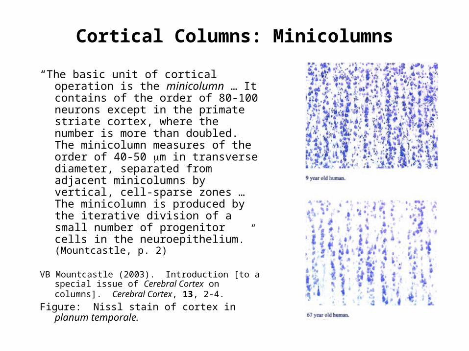
“The basic unit of cortical operation is the minicolumn … It contains of the order of 80-100 neurons except in the primate striate cortex, where the number is more than doubled. The minicolumn measures of the order of 40-50 m in transverse diameter, separated from adjacent minicolumns by vertical, cell-sparse zones … The minicolumn is produced by the iterative division of a small number of progenitor cells in the neuroepithelium.” (Mountcastle, p. 2)

VB Mountcastle (2003). Introduction [to a special issue of Cerebral Cortex on columns]. Cerebral Cortex, 13, 2-4.  

Figure: Nissl stain of cortex in planum temporale.

Columns: Functional 

Groupings of minicolumns seem to form the physiologically observed functional columns. Best known example is orientation columns in V1.

They are significantly bigger than minicolumns, typically around 0.3-0.5 mm.

Mountcastle’s summation:

“Cortical columns are formed by the binding together of many minicolumns by common input and short range horizontal connections. … The number of minicolumns per column varies … between 50 and 80. Long range intracortical projections link columns with similar functional properties.” (p. 3)

 

Cells in a column ~ (80)(100) = 8000

Sparse Connectivity The brain is sparsely connected. (Unlike most neural

nets.) A neuron in cortex may have on the order of 100,000

synapses. There are more than 1010 neurons in the brain. Fractional connectivity is very low: 0.001%.

Implications: • Connections are expensive biologically since they

take up space, use energy, and are hard to wire up correctly.

• Therefore, connections are valuable.• The pattern of connection is under tight control.• Short local connections are cheaper than long ones.

Our approximation makes extensive use of local connections for computation.

Network of Networks Approximation

We use the Network of Networks [NofN] approximation to structure the hardware and to reduce the number of connections.

 We assume the basic

computing units are not neurons, but small (104 neurons) attractor networks.

 Basic Network of Networks

Architecture:• 2 Dimensional array of

modules • Locally connected to

neighbors

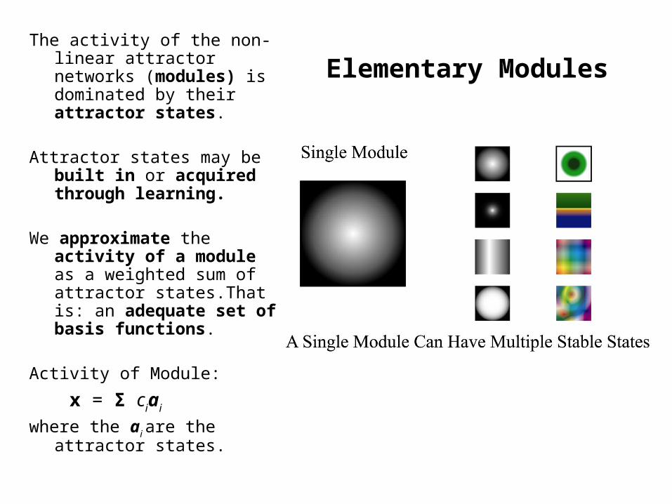
Elementary ModulesThe activity of the non-

linear attractor networks (modules) is dominated by their attractor states.

 Attractor states may be

built in or acquired through learning.

 We approximate the

activity of a module as a weighted sum of attractor states.That is: an adequate set of basis functions.

Activity of Module:

x = Σ ciai

where the ai are the attractor states.

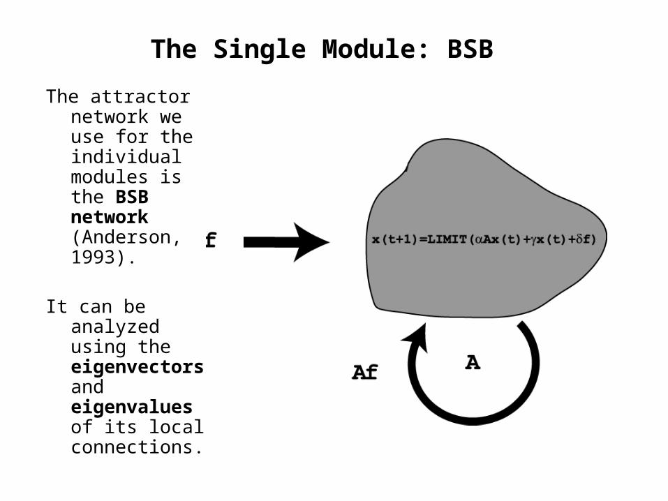
The Single Module: BSB The attractor

network we use for the individual modules is the BSB network (Anderson, 1993).

 It can be

analyzed using the eigenvectors and eigenvalues of its local connections.

Interactions between Modules

Interactions between modules are described by state interaction matrices, M.

The state interaction matrix elements give the contribution of an attractor state in one module to the amplitude of an attractor state in a connected module.

In the BSB linear region

x(t+1) = Σ Msi + f + x(t) weighted sum input ongoing from other modules activity

The Linear-Nonlinear Transition

The first BSB processing stage is linear and sums influences from other modules.

The second processing stage is nonlinear.

This linear to nonlinear transition is a powerful computational tool for cognitive applications.

 It describes the processing path taken by many

cognitive processes. A generalization from cognitive science: Sensory inputs (categories, concepts, words) Cognitive processing moves from continuous values

to discrete entities.

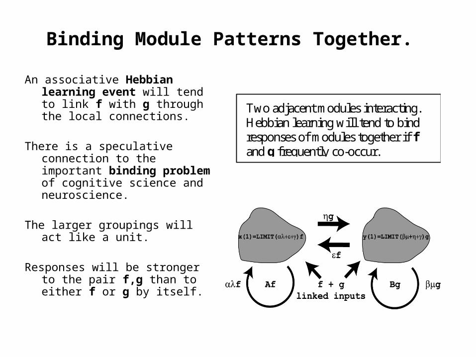
Binding Module Patterns Together. An associative Hebbian

learning event will tend to link f with g through the local connections.

 There is a speculative

connection to the important binding problem of cognitive science and neuroscience.

 The larger groupings will

act like a unit. Responses will be stronger

to the pair f,g than to either f or g by itself.

Two adjacent modules interacting. Hebbian learning will tend to bind responses of modules together if f and g frequently co-occur.

ScalingWe can extend this

associative model to larger scale groupings.

 It may become possible to

suggest a natural way to bridge the gap in scale between single neurons and entire brain regions.

 Networks >Networks of Networks > Networks of (Networks of Networks) >

Networks of (Networks of (Networks

of Networks))

and so on …

Interference Patterns

We are using local transmission of (vector) patterns, not scalar activity level.

We have the potential for traveling pattern waves using the local connections.

Lateral information flow allows the potential for the formation of feature combinations in the interference patterns where two different patterns collide.

Learning the Interference Pattern

The individual modules are nonlinear learning networks.

We can form new attractor states when an interference pattern forms when two patterns meet at a module.

Module Evolution

Module evolution with learning:

 

        From an initial repertoire of basic attractor states

 

        to the development of specialized pattern combination states unique to the history of each module.

Biological Evidence:Columnar Organization in Inferotemporal

Cortex

Tanaka (2003) suggests a columnar organization of different response classes in primate inferotemporal cortex.

 

There seems to be some internal structure in these regions: for example, spatial representation of orientation of the image in the column.

IT Response Clusters: Imaging

Tanaka (2003) used intrinsic visual imaging of cortex. Train video camera on exposed cortex, cell activity can be picked up.

 At least a factor of

ten higher resolution than fMRI.

 Size of response is

around the size of functional columns seen elsewhere: 300-400 microns.

Columns: Inferotemporal Cortex

Responses of a region of IT to complex images involve discrete columns.

 The response to a

picture of a fire extinguisher shows how regions of activity are determined.

 Boundaries are where

the activity falls by a half.

 Note: some spots are

roughly equally spaced.

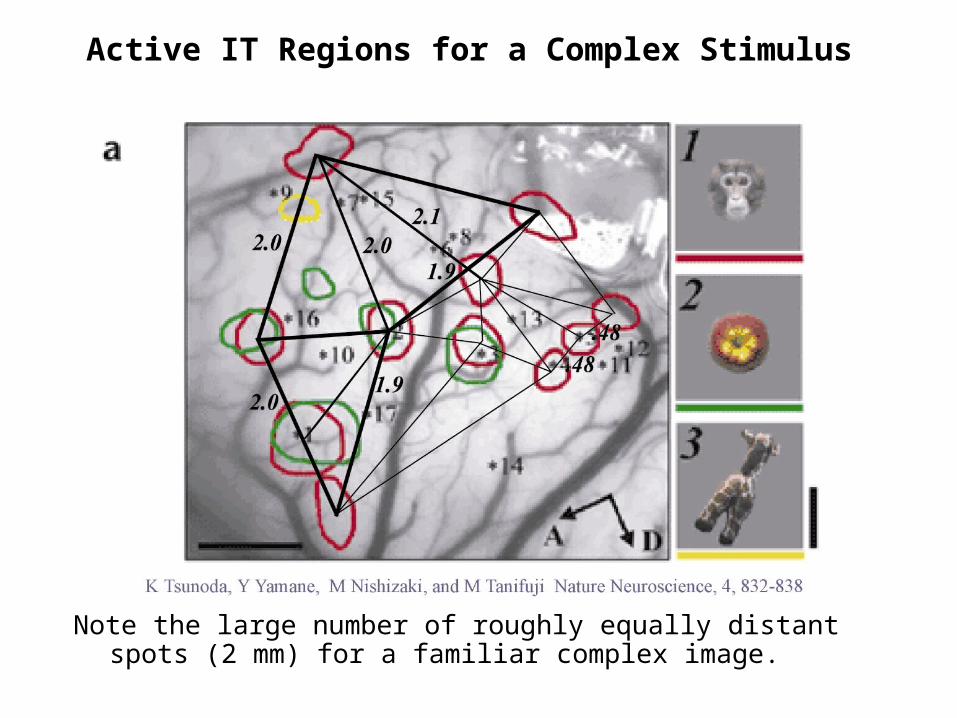
Active IT Regions for a Complex Stimulus

Note the large number of roughly equally distant spots (2 mm) for a familiar complex image.

Network of Networks Functional Summary.

• The NofN approximation assumes a two dimensional array of attractor networks.

• The attractor states dominate the output of the system at all levels.

• Interactions between different modules are approximated by

interactions between their attractor states.

• Lateral information propagation plus nonlinear learning allows formation of new attractors at the location of interference patterns.

• There is a linear and a nonlinear region of operation in both single and multiple modules.

• The qualitative behavior of the attractor networks can be controlled by analog gain control parameters.

Engineering Hardware Considerations

We feel that there is a size, connectivity, and computational power “sweet spot” at the level of the parameters of the network of network model.

 If an elementary attractor network has 104 actual neurons,

that network display 50 attractor states. Each elementary network might connect to 50 others through state connection matrices.

 A brain-sized system might consist of 106 elementary units

with about 1011 (0.1 terabyte) numbers specifying the connections.

 If 100 to 1000 elementary units can be placed on a chip

there would be a total of 1,000 to 10,000 chips in a cortex sized system.

 These numbers are large but within the upper bounds of

current technology.

A Software Example: Sensor Fusion

A potential application is to sensor fusion. Sensor fusion means merging information from different sensors into a unified interpretation.

 

Involved in such a project in collaboration with Texas Instruments and Distributed Data Systems, Inc.

 

The project was a way to do the de-interleaving problem in radar signal processing using a neural net.

 

In a radar environment the problem is to determine how many radar emitters are present and whom they belong to.

 

Biologically, this corresponds to the behaviorally important question, “Who is looking at me?” (To be followed, of course, by “And what am I going to do about it?”)

Radar

A receiver for radar pulses provide several kinds of quantitative data:

• frequency, • intensity, • pulse width, • angle of arrival, and • time of arrival.  The user of the radar system wants to know qualitative

information:  • How many emitters? • What type are they? • Who owns them? • Has a new emitter appeared?

Concepts

The way we solved the problem was by using a concept forming model from cognitive science.

 

Concepts are labels for a large class of members that may differ substantially from each other. (For example, birds, tables, furniture.)

 

We built a system where a nonlinear network developed an attractor structure where each attractor corresponded to an emitter.

 

That is, emitters became discrete, valid concepts. 

Human Concepts

One of the most useful computational properties of human concepts is that they often show a hierarchical structure.

 Examples might be: animal > bird > canary > Tweetie or artifact > motor vehicle > car > Porsche > 911. A weakness of the radar concept model is that it

did not allow development of these important hierarchical structures.

Sensor Fusion with the Ersatz Brain.

We can do simple sensor fusion in the Ersatz Brain.

The data representation we develop is directly

based on the topographic data representations used in the brain: topographic computation.

 Spatializing the data, that is letting it find a

natural topographic organization that reflects the relationships between data values, is a technique potential power.

We are working with relationships between values, not with the values themselves.

 Spatializing the problem provides a way of

“programming” a parallel computer.  

Topographic Data Representation

We initially will use a simple bar code to code the value of a single parameter.

The precision of this coding is low. But we don’t care about quantitative precision: We

want qualitative analysis.

Brains are good at qualitative analysis, poor at quantitative analysis. (Traditional computers are the opposite.)

Low Values Medium Values High Values

••++++•••••••••••••••••••••••••••••••••••••••••••••••••••••••••••••••••••++++•••••••••••••••••••••••••••••••••••••••••••••••••••••••••••••••••••++++••

DemoFor our demo Ersatz

Brain program, we will assume we have four parameters derived from a source.

 An “object” is

characterized by values of these four parameters, coded as bar codes on the edges of the array of CPUs.

 We assume local

linear transmission of patterns from module to module.

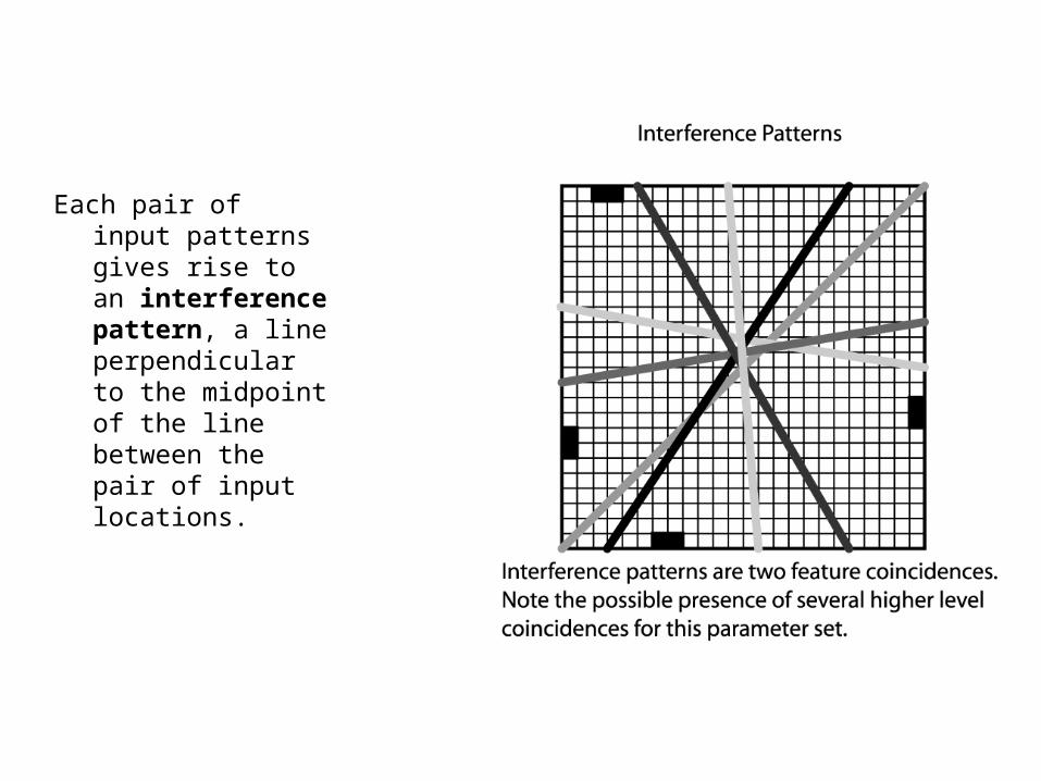
Each pair of input patterns gives rise to an interference pattern, a line perpendicular to the midpoint of the line between the pair of input locations.

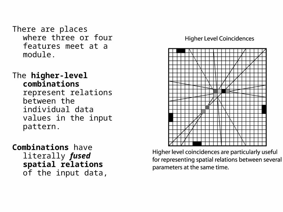
There are places where three or four features meet at a module.

 The higher-level

combinations represent relations between the individual data values in the input pattern.

 Combinations have

literally fused spatial relations of the input data,

Formation of Hierarchical Concepts.

This approach allows the formation of what look like hierarchical concept representations.

 Suppose we have three parameter values that are fixed for

each object and one value that varies widely from example to example.

 The system develops two different types of spatial data. In the first, some high order feature combinations are

fixed since the three fixed input (core) patterns never change.

 In the second there is a varying set of feature

combinations corresponding to the details of each specific example of the object.

 The specific examples all contain the common core pattern.

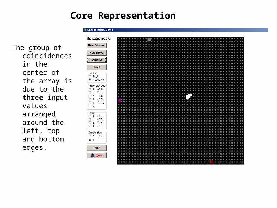
Core Representation

The group of coincidences in the center of the array is due to the three input values arranged around the left, top and bottom edges.

Left are two examples where there is a different value on the right side of the array. Note the common core pattern (above).

Development of A “Hierarchy” Through Spatial Localization.

The coincidences due to the core (three values) and to the examples (all four values) are spatially separated.

 

We can use the core as a representation of the examples since it is present in all of them.

It acts as the higher level in a simple hierarchy: all examples contain the core.

This approach is based on relationships between parameter values and not on the values themselves.

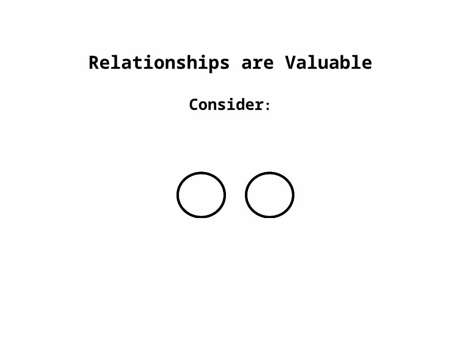
Relationships are Valuable

Consider:

Which pair is most similar?

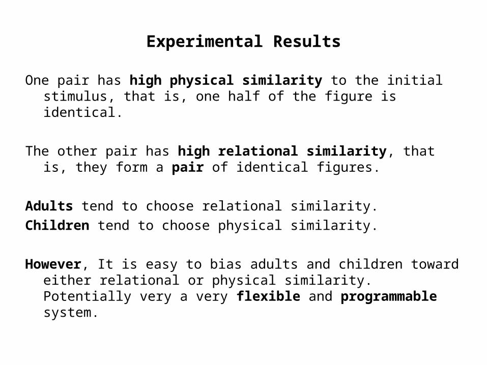
Experimental Results

One pair has high physical similarity to the initial stimulus, that is, one half of the figure is identical.

The other pair has high relational similarity, that is, they form a pair of identical figures.

Adults tend to choose relational similarity.

Children tend to choose physical similarity.

However, It is easy to bias adults and children toward either relational or physical similarity. Potentially very a very flexible and programmable system.

Cognitive Computation:Second Example - Arithmetic

• Brains and computers are very different in the way they do things, largely because the underlying hardware is so different.

• Consider a computational task that humans and computers do frequently, but by different means:

– Learning simple arithmetic facts

The Problem with Arithmetic

• We often congratulate ourselves on the powers of the human mind.

• But why does this amazing structure have such trouble learning elementary arithmetic?

• Even adults doing arithmetic are slow and make many errors.

• Learning the times tables takes children several years and they find it hard.

The Problem with Arithmetic

At the same time children are having trouble learning arithmetic they are knowledge sponges learning – Several new words a day.– Social customs.– Many facts in other areas.

Association

In structure, arithmetic facts are simple associations.

Consider multiplication:

(Multiplicand)(Multiplicand) Product

Multiplication• These are not arbitrary associations.

• They have an ambiguous structure that gives rise to associative interference.4 x 3 = 124 x 4 = 164 x 5 = 20

• Initial ‘4’ has associations with many possible products.

• Ambiguity causes difficulties for simple associative systems.

Number Magnitude

• One way to cope with ambiguity is to embed the fact in a larger context.

• Numbers are much more than arbitrary abstract patterns.

• Experiment:– Which is greater? 17 or 85– Which is greater? 73 or 74

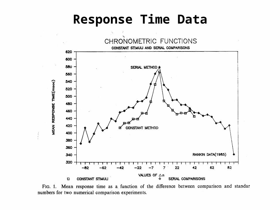
Response Time Data

Number Magnitude

It takes much longer to compare 74 and 73.

When a “distance” intrudes into what should be an abstract relationship it is called a symbolic distance effect.

A computer would be unlikely to show such an effect. (Subtract numbers, look at sign.)

Magnitude Coding

Key observation: We see a similar pattern when sensory magnitudes are being compared.

Deciding which of – two weights is heavier, – two lights is brighter, – two sounds is louder – two numbers is bigger

displays the same reaction time pattern.

Magnitude Coding

This effect and many others suggest that we have an internal representation of number that acts like a sensory magnitude.

Conclusion: Instead of number being an abstract symbol, humans use a much richer coding of number containing powerful sensory and perceptual components.

Magnitude Coding

This elaboration of number is a good thing. It

– Connects number to the physical world.

– Provides the basis for mathematical intuition.

– Responsible for the creative aspects of mathematics.

Model Makes Small Mistakes, Not Big Ones

Model used a neural network based associative system.

Buzz words: non-linear, associative, dynamical system, attractor network.

The magnitude representation is built into the system by assuming there is a topographic map of magnitude somewhere in the brain.

First Observation about Arithmetic Errors

Arithmetic fact errors are not random.

• Errors tend to be close in size to the correct answer.

• In the simulations, this effect is due to the presence of the magnitude code.

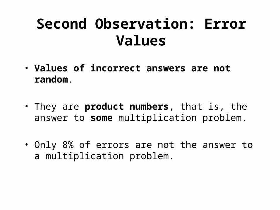
Second Observation: Error Values

• Values of incorrect answers are not random.

• They are product numbers, that is, the answer to some multiplication problem.

• Only 8% of errors are not the answer to a multiplication problem.

Human Algorithm for Multiplication

The answer to a multiplication problem is:

1. Familiar (a product)

2. About the right size.

Human Algorithm for Multiplication

• Arithmetic fact learning is a memory and estimation process.

• It is not really a computation!

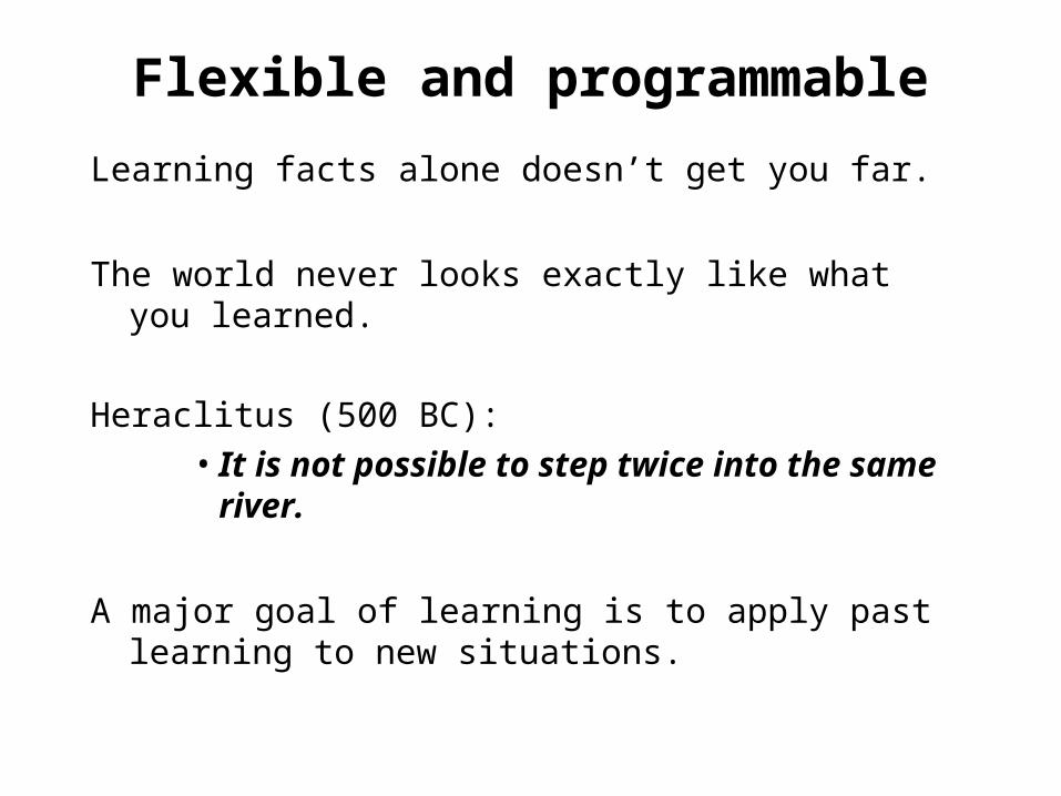
Flexible and programmable

Learning facts alone doesn’t get you far.

The world never looks exactly like what you learned.

Heraclitus (500 BC):•It is not possible to step twice into the same river.

A major goal of learning is to apply past learning to new situations.

Getting Correct What you Never Learned: Comparisons

Consider number comparisons: Is 7 bigger than 9?

We can be sure that children do not learn number comparisons individually.

There are too many of them.

– About 100 single digit comparisons– About 10,000 two-digit comparisons– And so on.

Magnitude

• We now see the usefulness of the “sensory” magnitude representation.

• We can use magnitude to do computations like number comparisons without having to learn special cases.

• A generalization of the multiplication simulation did comparisons of number pairs it had never seen before. (Without further learning.)

Implications

We have constructed a system that acts like like logic or symbol processing but in a limited domain.

It does so by using its connection to perception to do much of the computation.

These “abstract” or “symbolic” operations display their underlying perceptual nature in effects like symbolic distance and error patterns in arithmetic.

Connect perception to abstraction and gain the power of each approach

• Humans are a hybrid computer.

• We have a recently evolved, rather buggy ability to handle abstract quantities and symbols.

• (only 100,000 years old. We have the alpha release of the intelligence software.)

• We combine symbol processing with highly evolved, extremely effective sensory and perceptual systems.

• Realized in a mammalian neocortex.

• (over 500 million years old. We have a late release, high version number of the perceptual software.)

• The two systems cooperate and work together effectively.

Connect perception to abstraction and gain the power of each approach

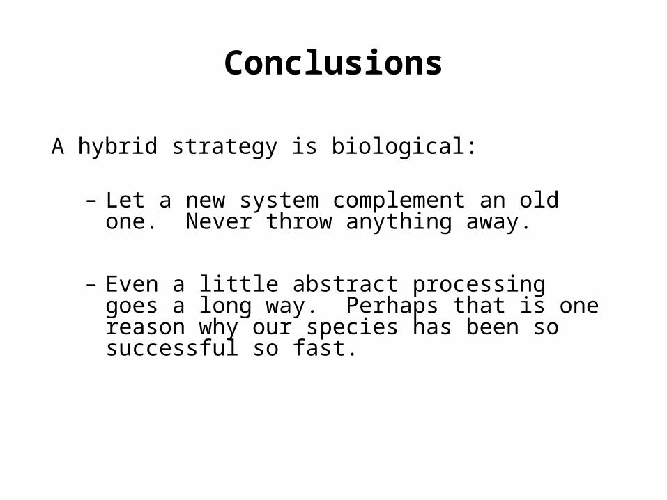
Conclusions

A hybrid strategy is biological:

– Let a new system complement an old one. Never throw anything away.

– Even a little abstract processing goes a long way. Perhaps that is one reason why our species has been so successful so fast.

Conclusions

Speculation: Perhaps digital computers and humans (and brain-like computers??) are evolving toward a complementary relationship.

• Each computational style has its virtues: – Humans (and brain-like computers): show flexibility, estimation, connection to the physical world

– Digital Computers: show speed, logic, accuracy.

• Both styles are valuable. There is a valuable place for both.