J . Fluid Me&. (1987), vol. 178, pp. 53-71

Printed in Ureai Britain

53

A boundary-layer analysis of Rayleigh-Benard convection at large Rayleigh number

By JAVIER JIMENEZ IBM Scientific Centre, P w o Castellana 4, 28046 Madrid, Spain

AND JUAN A. ZUFIRIAt School of Aeronautics, Universidad PolitBcnica, 28040 Madrid, Spain

(Received 20 March 1986 and in revised form 23 September 1986)

A boundary-layer analysis is presented for the two-dimensional nonlinear convection of an infinite-Prandtl-number fluid in a rectangular enclosure, in the limit of large Rayleigh numbers. Particular emphaais is given to the analysis of the periodic boundary layers, and on the removal of the singularities that appear near the corners of the cell. It is argued that this later step is necessary to ensure the correctness of the boundary-layer assumptions. Numerical values are obtained for the heat transfer and stress characteristics of the flow.

1. Introduction It is generally accepted by now that natural convection in the Earth’s mantle is

the driving mechanism for plate tectonics. This has produced a renewed interest in the study of natural convection in enclosures, resulting in numerous studies of simplified models which may throw light on the underlying mechanism controlling the behaviour of the mantle. Perhaps the simplest of those models is a Boussinesq fluid confined between stress-free boundaries and heated from ,below. Even if the direct relation to mantle convection is doubtful, especially with the aasumption of the stress-free upper boundary, this model haa the virtue of simplicity and corres- ponds to a geometry which has been studied for a long time at different regimes (Rayleigh 1916; Chandrasekhar 1961 ; Brindley 1967).

The range of parameters that is of interest for the mantle is that of an essentially infinite Prandtl number, Pr x loes, and a relatively high Rayleigh number, Ra x lo6 (Turcotte & Oxburgh 1967). Under those conditions, viscosity is dominant, and the preferred mode of convection is believed to be steady two-dimensional rolls (Strauss 1972; Jones, Moore & Weiss 1976), formed by a central isothermal core and thin thermal layers (Turcotte 1967). This will be the case considered here.

Except for the original motivation of the mantle convection, we will treat the problem as one of intrinsic theoretical importance, and we will be interested mostly in developing methods of solution for it, in the limit of large Rayleigh numbers, and in clarifying the possible singularities that appear on the asymptotic regime.

Numerical simulations of the flow have been published by Moore & Weiss (1973) and McKenzie, Roberts & Weiss (1974), using finite differences schemes, and by Veronis ( 1966), using spectral methods. More complicated models, including temperature-dependent viscosity and other real fluid effects can be found in (Torrance

t Present address : Applied Mathematics Department, California Institute of Technology, Pasadena, CA 91125, USA.

54 J . Jimenez and J . A . Zu&a

& Turcotte 1971a, b; Olson & Yuen 1982), and a numerical scan of different convection regimes including different Prandtl numbers and unsteady effects is given by Arter (1985).

While these studies are important displaying the ‘phenomenology’ of the problem, they do not provide much understanding of the physics behind the phenomena. Our belief is that simpler models have to be understood before dealing with the more complicated cases which are representative of real life.

Moreover, classical finite difference, finite element and spectral methods become increasingly inaccurate and difficult to use for large Rayleigh number, owing to the need to resolve the thermal boundary layers.

The first asymptotic treatment of the problem is due to Turcotte (1967) and Turcotte & Oxburgh (1967), who gave a good analysis of the overall flow structure but used a relatively crude approximation for the thermal boundary layers them- selves. Later Roberts (1979) and Olson & Corcos (1980) presented improved boundary- layer analysis, but we believe them to be incorrect (see $6). Moreover, none of these authors pay attention on the problem of resolving the singularities that appear in the limit of infinitely thin boundary layers. Even if these singularities do not have a large influence in the computation of integral quantities like the total heat flow, they are certainly locally important for properties such as the topography of the free surface or the maximum heat flux. Even more important, until it has been shown that these singularities can be removed by a local analysis and integrated into a uniformly valid solution for the complete problem, it is not guaranteed that the solution actually exists, and that the assumptions that lead to the boundary-layer approximations are justified. We will come back to this problem below.

As a further demonstration that the analysis of even this comparatively simple model is still not satisfactory, we will see later that the present estimates for the total heat transfer coefficient for a complete cell vary among different authors by up to 30 yo, without a clearly defined best value.

Motivated by these considerations, we have developed a new boundary-layer analysis for the stress-free Rayleigh-BBnard convection in the limit mentioned above, paying special attention to the cyclic thermal boundary layers, and to the resolution of the singularities that appear, in the asymptotic limit, near the corners of the cell. In the next section we state the problem and present the solution for the isothermal core. The boundary layers are treated next, and $5 contains the analysis of the corners.

2. Statement of the problem Our model consists of a Boussinesq fluid with infinite Prandtl number moving

under convective forces between two horizontal surfaces that are kept at different constant temperatures. Let Tb and T, be the temperatures of the lower and upper surfaces, and let Tb > T, (see figure 1). We are interested in flows with a two- dimensional structure of cells arranged periodically in the s-direction. The depth of each cell is hn, and its length Ahn. Under these assumptions the dimensionless equations that describe the motion of the fluid can be written, in terms of the stream function and the temperature, as (Olson & Corcos 1980)

A boundary -layer analysis of Rayleigh-Bdnard convection 56

3 T= T,

h T = Tb Arh

FIWRE 1. Geometry of the flow.

where the dimensionless variables are defined aa

and !P and (X, Y) are respectively the physical stream function and coordinates. The Rayleigh number is de&ed aa

d T b - T u ) ha V K

Ra = 3

where K is the thermal diffusivity, g is the acceleration of the gravity, v is the kinematic viscosity, and a is the coefficient of thermal expansion, all aasumed constant. The parameter a, which turns out to be of order one, is defined aa

a = ($$ and Nu is the Nusselt number that we define aa

(3)

Here Q is taken to be the total heat flux through the upper surface of each cell. A priori, Q is unknown, and has to be found aa a part of the problem but, as we will see below, the use of this parameter introduces important simplifications in the resolution of the problem. U, is a characteristic velocity of the flow, defined as

u, = K (y. h a

When the Rayleigh number is large, the flow in each cell is formed by an isothermal core surrounded by a thin thermal boundary layer that carries all the heat, and whose thickness is of order Raf (Turcotte 1967). The boundary layer is heated by conduction at the bottom, rises by buoyancy forming vertical plumes, and releases its heat through the upper surface by conduction. After that, the cold layer sinks, because of the negative buoyancy, closing the cycle.

The axes of the plumes separate the cells and are axes of symmetry of the problem.

56 J . Jimenez and J . A . Zujria

They act as adiabatic vertical walls, from the thermal point of view, and as free surfaces from the dynamical point of view. Also, we will assume that the two horizontal surfaces are stress free.

The boundary conditions that complete the problem are

From the analysis of equations (l), (6) for large Ra, i t can be shown that the solution in the core admits the following asymptotic expansion

where e = (Ra/cr)i. To study the flow inside the plumes we introduce a transverse stretched coordinate x by introducing 2 = ex, and the asymptotic form of the solution becomes

(8)

The coupling between the core and the plumes can be obtained by integrating the

1 G(2, Y) = €Go@, Y) +e2G1(2, Y) +0(e3),

a(?, y) = a,($, y) + &2, y) + 0 ( e 2 ) .

momentum equation across the plumes for constant y.

where p(Ra) is chosen such that p(Ra) + O and ,u(Ra)/e+ 00 as Ra+ 00. I n this limit, the leading term of the expansion for (9) becomes

where y is the ratio between the heat carried by the ascending plume and Q. Since, in the first approximation, there is no heat transfer between the core and the plumes, y is independent of y.

The uniform temperature in the core 8, can be determined by a contour integral around the cell (G. M. Corcos, private communication),

A boundary-layer analysis of Rayleigh-Bdnard convection 57

where 8, is the temperature at the cell boundaries. It follows from symmetry arguments that 8, = ?j and y = 4.

At this point we can write the equation for the leading term of the isothermal motion of the core as

with the boundary conditions V4$, = 0, (12)

where the only parameter is A, the aspect ratio of the cell. We have integrated this equation numerically by using a pseudospectral method

(Jimenez t Zufiria 1984). It can be shown, by a local analysis of the equation, that the vorticity becomes singular at the four corners of the cell, and it was necessary to isolate these singularities from the spectral expansion, in order to get a good convergence of the numerical method. The local behaviour of the stream function and of the vorticity near the corners is given by

I r; $, = - (sin@-sin@), 2

w = -V2yF0 = r-i sin@,

where r and 4 are polar coordinates centred at the corner. Plots of the streamlines for two different cells and of the vorticity distribution are

given in figure 2. The vorticity is dominated by the singularities at the corners, all of which are equivalent in this approximation because of the symmetries of the problem. Note that the variables obtained here are dimensionless, and cannot be related to physical quantities until the scale factor is computed from the thermal behaviour of the boundary layers. In return, the core flows discussed here are universal and can be computed in terms of the elongation A.

3. Thermal boundary layers To describe the evolution of the thermal boundary layers we introduce a new system

of coordinates (a,n), where a is a downstream coordinate in the layer and n is a transverse coordinate, normal everywhere to the wall and measured inward from the boundary (figure 3). Note that 8 runs around the cell and is really formed by patching together the four sides of the cell into a single continuous line. We will assume that, at the points of suture that correspond to the corners, the temperature in the boundary layer is continuous, except at the wall where the boundary conditions impose discontinuities. This is equivalent to the assumption that there exists a corner region, small with respect to the dimensions of the cell, in which the velocity

58 J . Jimenez and J . A . Zufiria

FI~URE 2. Streamlines and vorticity distribution for the isothermal core flow in rectangular cells. (a) Streamlines, A = 1.5, distance among streamlinea is A@ = -7.2 x 10-8. (a) Streamlines, A = 2.5.A@ = -6 x lo-*; note how flow separates into almost independent eddies. (c) Vorticity, A = 1.5, maximum dimensionless vorticity represented in plot is -3.32.

A boundary-layer analysis of Rayleigh-BCnard convection 59

e = i 3

1 e=o

FIGURE 3. Coordinate system and general geometry for analysis of boundary layers.

distribution is smooth and without recirculation, and where the temperature may be assumed to be passively convected along the streamlines. The validity of this assumption will be justified in $5, when we treat the corner flow in detail.

For large Ra, and stream-free boundaries, the velocity within the boundary layer depends, in the first approximation, only on 5. Rescaling the transverse coordinate with (a/Ra)t, to have a thickness of order unity, the equation for the leading term of the temperature distribution t90(5, n) in the layer is

At the boundary (n = 0) the temperature is known at the segments corresponding to the top and bottom surfaces, and the heat flux has to vanish at the segments corresponding to the two vertical plumes. As n-+co, on the other hand, the temperature distribution has to match to the isothermal core and so+& These conditions complete the problem.

Equation (15) can be simplified by introducing the Crocos stretching

I f = U(s)ds, 0

U(5) dn = tU(s ) n,

which reduces (15) to the heat equation,

The temperature distribution in the layer can now be written in terms of the temperature at the wall and of the temperature distribution in an upstream

3 FLX 178

60 J . Jimenez and J . A . Zujiria

transverse section. If 8, is the temperature at the wall and g ( 7 ) = ao(0,a) , the temperature anywhere in the boundary can be expressed as

+'r 'IV('gp) exp-fdp. (18) x2 0 P2 P

This expression can be simplified by using the fact that the problem is periodic, with each period corresponding to one loop, and by moving the initial section several periods upstream. If we add N loops to the previous equation, it becomes

exp--dp, a2 (19) P

where L is the length of a single loop of the boundary layer in stretched variables, r

8, is a periodic function with period L. Taking now the limit N+m, the first integral in (19) vanishes and the equation simplifies to

which is a function only of the temperature at the wall. From the boundary conditions we know 8, on sides 1 and 3 (top and bottom of

the cell). To determine i t on the other two sides, we derive the expression for the heat flux at the wall by differentiating (21), and equate it to zero along the plumes;

This is an integral equation which should hold on sides 2 and 4, and whose solution allows us to compute 8, along those sides and, through (21), the temperature everywhere in the boundary layer. Notice that the equation is not homogeneous because 8, = 1 on the lower surface.

In particular, the dimensionless heat flow carried by the plumes can be expressed in terms of 8, as rF

where t; represents the section in which the flux is computed, and the equation has to be independent of 5. Since the only unknown in (23) is now (T, this equation can be used to compute (T and, therefore, to fix the physical scale of the whole problem.

Note that the inner integral in (23),

5

5-t (@w(7)-@o)d7,

A boundary-layer analysis of Rayleigh-BCnurd convection 61

is a periodic function of q with zero mean value. This is LL necessary condition for the integral in (22) to be convergent, and constitutes, in fact, a new proof for equation (11) .

In summary, the solution procedure for the complete problem of the flow in the cell is the following. For a given aspect ratio A, we compute the flow in the isothermal core, except for the scale factor cr. This allows us to compute the velocity near the walls and the stretched lengths of the four cell sides ( l , , l , , I , = I , , 1, = 1 2 ) . We then solve the integral equation (22) to compute the temperature distribution along the axes of the vertical plumes and use (23) to determine the scale factor cr, closing the problem. If desired, (21) can be used to compute the temperature distribution anywhere in the boundary layer.

4. Numerical solution of the thermal problem The wall temperature 8, and the heat flux to the wall vary discontinuously when

the thermal boundary layer approaches the corners of the cell. To solve numerically the integral equation (22), these discontinuities have to be taken explicitly into account. This is especially true in the evaluation of integral (23), which is needed to compute the scale factor cr. As mentioned above, this integral makes sense only if the average value of the inner integral is identically zero, and small numerical integration errors can lead to large errors in the final result.

Downstream from the corners between the sides 2, 3 and 4, 1, the temperature is fixed by the boundary condition. Since the boundary-layer equation is parabolic, this means that the temperature itself is discontinuous. It follows from the heat equation (17) that, downstream from these discontinuities, a@,/aq cc E-i, which is equivalent to a@,/an cc 5-f. A t the other two corners, the temperature is continuous, but the temperature changes as @, (equivalent to st ) as it leaves those corners.

To minimize the numerical accuracy problems produced by these discontinuities, we isolate the leading term of the singular behaviour of the wall temperature distributions along the vertical plumes. Taking into account the symmetries of the problem,

(24 )

@wp(.g) = 1 - A 7 h - q 7 ) ,

@,,(El = A7i+e(74),

7 = [ - - 1 1 , r4 = ~ - 1 , - 1 2 - 1 3 , ~

where O ( 7 ) is continuous and O ( d ) as 7+0. If we substitute these expressions in (22) and integrate the singular parts, we get the heat flux on side 2,

The last integral in this equation is not singular, but for numerical purposes, it is better to express it as a sum over all the L-period loops. With the change of coordinates E-q = k L - y we get

3-2

62 J . Jimenez and J . A . Zujiria

which, using (24) becomes

where the function W is defined as

- sin-’ 1

k-l [ z - 1 + kL/l,]i W(2) = 2 E {

All the series in these equations converge very slowly, but the asymptotic behaviour of their ‘tails’ is easy to estimate, and can be used to accelerate the numerical summation. In this way, we are able to compute the sums to 15 significant digits with only 40 terms.

All the terms in equations (25)-(28) are now well behaved in the whole interval (0, I t ) . The equation can be solved numerically by satisfying it at n+ 1 equidistant points in the interval, including the two end-points. The first n independent variables are the values of e(7) at 7t = iZ2/n, i = 1,2, ..., n. The value of 8(0) is zero by construction, and its place as independent variable is taken by the coefficient A . Note that, at 7 = 0 the third term in (25), vanishes without singularity, and the equation can be used at that point without special precautions.

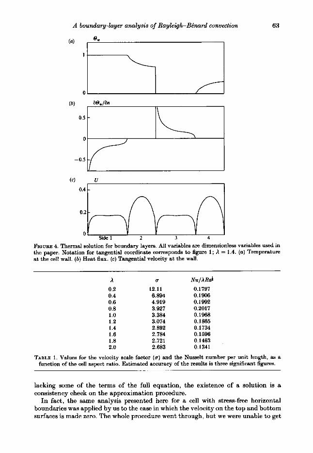
Figure 4 shows the wall temperature, the heat flux to the wall, and the tangential velocity at the wall computed for a particular value of the elongation. The singularities of the heat flux, and the behaviour of the temperature and the velocity near the corners are all clearly visible. Table 1 gives the Nusselt number per unit length computed as a function of the cell elongation. The numerical accuracy cited in the caption to the table is mainly limited by the number of harmonics (in this case 20) used in the spectral calculation of the core flow. Figure 5 shows the temperature distribution across the boundary layer a t several points along the rising vertical plume and the top horizontal surface. It shows the approach to the self-similar temperature distributions at the end of both sides, and the formation of a hot ‘asthenosphere’ underneath the top boundary. Because of the symmetry of the problem, the two other sides are symmetric to the ones shown.

5. Cornerflow The boundary-layer solution that we have considered up to now is valid everywhere

except near the corners of the cell, where both the vorticity and the heat flux become infinite. We develop in this section a local analysis for these regions, with a view to resolving the infinities, and constructing an uniformly valid solution. Besides the ‘practical’ result of providing a number for the maximum velocity and heat flux, this has the effect of showing that a solution can be constructed, and serves as a check for the assumptions made on the structure of the flow and, in particular, for the separation into a core flow and a boundary layer.

It will be shown below that the equation for the stream function in the corner region is elliptic and has inhomogeneous boundary conditions along the walls and at infinity. Under those conditions, it is not guaranteed that a solution exists, and the existence of a solution is itself a proof of the consistency of the boundary conditions. Since, in our problem, those conditions result from the solution of approximate equations

A boundary -layer analysis of Rayleigh-Bdnard convection 63

(4 U r I

FIQURE 4. Thermal solution for boundary layers. All variables are dimensionless variables used in the paper. Notation for tangential coordinate corresponds to figure 1 ; A = 1.4. (a) Temperature at the cell wall. (b) Heat flux. (c) Tangential velocity at the wall.

A 0.2 0.4 0.6 0.8 1 .o 1.2 1.4 1.6 1 .a 2.0

U

12.11 6.894 4.919 3.927 3.384 3.074 2.892 2.784 2.721 2.683

N ~ ~ A R ~

0.1797 0.1906 0.1992 0.2017 0.1908 0.1865 0.1734 0.1596 0.1463 0.1341

TABLE 1. Values for the velocity scale factor (a) and the Nusselt number per unit length, as a function of the cell aspect ratio. Estimated accuracy of the results is three significant figures.

lacking some of the terms of the full equation, the existence of a solution is a consistency check on the approximation procedure.

In fact, the same analysis presented here for a cell with stress-free horizontal boundaries was applied by us to the case in which the velocity on the top and bottom surfaces is made zero. The whole procedure went through, but we were unable to get

J. Jimenez and J . A . Zujiria

x = o

0.5

FIGURE 5. Temperature profile across the boundary layers; A = 1.4. ( a ) Vertical rising plume. ( b ) Top horizontal surface. Flow is from left to right in both cases. Note formation of a hot asthenosphere underneath the top boundary.

a consistent solution for the corners. We considered that to bc an indication that the boundary-layer approximation is not appropriate in that case.

We will concentrate here on the corner between sides 2 and 3 (figure 6). It is clear from the symmetry of the problem that the corner 4-1 is equivalent to this one, while the other two are different, but can be analysed in a similar way.

The corner region is actually a part of the thermal boundary layer, where the buoyancy forces are important but, now, the velocity can no longer be considered approximately constant. As a consequence, the corner is defined as a region in which the buoyancy and viscous forces are in balance. This occurs at a linear scale of O(Ra-t), which is larger than the thickness of the thermal boundary layer, which is O(Ra-4). Consider the following stretching

I r* = (Racr2/33)tr,

+* = (Rau2/33)b+,

0* = /3(0-0,),

and 0, is the temperature a t the plume axis when the plume reaches the corner, which is known from the boundary-layer solution computed above.

A boundary-layer analysis of Rayleigh-Be'nard convection 65

't / *

FIQURE 6. Coordinate system and geometry of the corner.

With this stretching, equations (1 ) become

The first consequence of these equations is that, as Ra+ 00 the heat conduction can be neglected inside the corner. In fact, it is only important in an infinitely thin layer, O(Raf) , near the horizontal top surface, where the temperature has to fall to zero to mtisfy the boundary condition. Inside this layer the temperature variation is large but, since the layer is horizontal, buoyancy forces are negligible and the stress-free condition can be applied across it. Everywhere else the temperature is constant along the streamlines and depends only on the stream function, @* = @*(+*). This function is determined by matching upstream to the temperature distribution in the thermal boundary layer.

In the limit of large Ra, by the time that the plume reaches the upper corner, its temperature distribution has already attained the self-similar value

where the stars have been dropped to simplify the notation. Introducing this distribution in (31), we obtain a single equation for the stream function

We know the values of the stream function and the vorticity both at the walls and at infinity. On the walls, $ = w = 0. As we move away from the corner, the inner solution that we are considering here has to match the behaviour of the outer solution

66 J . Jimenez and J . A . ZuJiria

as it approaches the corner. Introducing polar coordinates, this behaviour is given by (14) everywhere except near the vertical wall. There, we find the vertical plume, within which the stream function and the velocity are still given in first approxi- mation by (14) but the vorticity is not. This is also clear from the fact that the vorticity distribution in (14) does not tend to zero as it approaches x = 0.

While it would be possible to impose the boundary condition far enough from the corner that the vertical thermal layer could be modelled as a discontinuity at the vertical wall and that (14) could be used everywhere except strictly at x = 0, i t is more efficient to form a composite vorticity distribution that includes approximately the effects of the buoyancy forces inside the plume. Integrating the momentum equation across the plume in the same way as in (9), and using the temperature distribution (32) , we get a vorticity distribution in the plume

where v is the vertical velocity a t the plume, obtained from (14). This vorticity distribution vanishes at the wall and matches (14) away from it. From both solutions we can construct a uniformly valid approximation that can be used as a boundary condition a t large y,

where 9 is given by (14) and decreases away from the wall. Note that as r increases, the thickness of the thermal layer decreases, as expected.

Neither (33) nor the boundary conditions contain any parameter, and the solution, once found, is universal. We have obtained it numerically using a naive first-order difference scheme in $ and w , and a variable mesh designed to deal with the infinite domain. Both the difference scheme and the mesh generation are described in the Appendix. The solution is presented in figure 7 , with the sign of the vorticity reversed for clarity. Note that the singularity of the vorticity in the outer flow is smoothed here to a finite peak.

In the inner region very close to the corner, the velocity gradients become large, the viscous terms are dominant, and the flow becomes irrotational,

The effect of the corner is to adapt this locally irrotational flow to the outer solution in the isothermal core. This is shown in figure 8, which shows the variation of the tangential velocity along both walls in the vicinity of the corner. The inner region shows the linear slope characteristic of (36) , while the outer part matches the square root behaviour of (14).

The evolution along the top horizontal boundary is specially interesting. Near the corner, this wall supports a thermal layer which is thin even at the scale of the corner region, and can be modelled by the boundary-layer equation (15). The boundary-layer coordinates are now s = z and n = - y, and from (36) , U(S) = Ks. The Crocos stretched variables are then E = ?jKa2, and 7 = ?jKsn, and the heat flux in Crocos and physical variables is related by

A boundary-layer analysis of Rayleigh-Be'nurd convection 67

0 4 8

8

FIQURE 7. Local solution for corner flow corresponding to corners 2-3 or 1 4 in figure 1. (a) Streamlines. Incoming thermal plume rises on the left; free surface on top. Distance among streamlines, A+* = - 1.85. (b ) Vorticity. Note how the singularity in the outer core flow is smoothed to a finite peak. Maximum vorticity, w* = -0.296.

68 J . Jimenez and J . A . ZuJria

10

u*, 0.

1

0.01 / 0.1 1 10 100

x*, Y*

FICHJRE 8. Tangential velocity at the walls of the corner solution as a function of the distance to corner. Note transition between inner and outer solutions. Last point to the right represents the edge of the numerical mesh in both cases. 0, u*(z*): A, u*(y*).

In the Crocos variables, the thermal layer sees just a discontinuous temperature jump from 0 = 1/& which is the value of (32) at the wall, to the boundary value 0 = 0. The heat flux corresponding to this jump is

Therefore, the heat flux is also made finite with a characteristic value given by (38). An approximate value for K , derived from the numerical solution is 0.4.

6. Discussion and conclusions We have presented a boundary-layer analysis of a simple model of natural

convection between stress-free surfaces in the limit of infinite Prandtl number and large Rayleigh number. An important result of the analysis is the Nusselt number per unit length (table l ) , which can be used to compare our results to those of previous investigators. This is done in figure 9 which shows that previous results disagree substantially with each other and with the values derived in this paper. It is our belief that the model has never been treated with the required precision.

Moore & Weiss (1973) use a finite-difference scheme on a uniform grid, with Pr = 100 and Ra = 15000-30000. Their densest grid contained 48 horizontal inter- vals, which are not sufficient to resolve a boundary layer of order Ra-: (the authors incorrectly use as their estimate for thc boundary-laycr thickness (Ra/Ra,)-:, where Ra, 657 is the critical value for stability). Vcronis' (1966) spectral calculation suffers from a similar lack of resolution, and that is also true of most of the other purely numerical calculations. As pointed in $ 1 , it is very difficult to reach adequate resolution a t large Rayleigh numbers without taking special precautions at the boundary layers.

The asymptotic analysis of Turcotte (1967) is essentially correct, but he makes no attempt to include treatment of the thermal boundary layers, and his numerical

A boundary-layer analysis of Rayleigh-Be'nard convection 69

0.3

0.2

0.1

Nu A R d ~

.

.

'

0.4 I t

t 0 1 2

A

FIGURE 9. Nuaselt number per unit length as a function of cell aspect ratio. Solid line, this paper; 0, Roberts 1979; 0, Olson & Corcos 1980; A, Veronis 1965; V, Strauss 1972; 0, Moore & Weiea 1973; 0, Turcotte & Oxburgh 1967.

results can only be considered as rough approximations. Olson & Corcos (1980) state the equation for the boundary layer correctly but, in their solution, they assume that the vertical plume satisfies the self-similar profile derived from a point source, and thus neglect the effect of closed streamlines. This is only approximately true. Moreover, they do not take into account explicitly the effects of the singularities in the flow, and their numerical results have low accuracy. Roberts (1979) recognizes the effect of periodic conditions in the boundary layers, and tries to solve the equations by a spectral method modified to take into account the discontinuities in temperature. However, he uses auxiliary discontinuous functions which do not satisfy the equations across the discontinuities, and his numerical results are wrong.

We believe that our analysis provides a correct complete solution for the flow. The local analysis of the corners gives both numerical values for maximum stress and heat flow, and shows that a consistent uniformly valid solution can be constructed. This is always important in elliptic problems, like this one, in which existence is not guaranteed and serves to check the validity of the asymptotic assumptions. As pointed out before, we have found cases in which this does not appear to be possible, probably pointing to a failure of the boundary-layer approximation.

Finally, our analysis includes a semi-analytical study of a thermal boundary layer with closed streamlines. This is a problem that has not been extensively treated in the literature.

One of us (J . A.Z.) was supported in part during his work by a fellowship from the Spanish Department of Education under the program of Formation of Research Personnel. The computing was carried out on the 370/158 computer of the IBM Madrid Scientific Centre.

70 J . Jimenez and J . A . Zujria

Appendix. Numerical treatment of comer equation Equation (33) can be rewritten in terms of the vorticity as

V 2 $ + W = 0,

The difference scheme that we have used to approximate the differential operators is the following,

where h . = x - x . = y - y 2 f 2-1 2 2-1'

A similar scheme has been used to discretize V2w. The mesh was chosen to be sparser in the outer part of the region, where the

gradients are smaller, and was generated to keep the integration error approximately constant in that region. The worst truncation error is the one associated with the discretization of the Vz$ operator, and is given by

Using (14) to estimate the behaviour on $ in the outer region, and taking into account that the integration error in $ is proportional to h27, we find that the condition for the error to be constant is equivalent to h2Ah cc xi. It is easy to see that this condition is approximately satisfied by h, cc k!. The actual law used was

(A 4) h, = 0.1 ki,

which corresponds to an actual integration error of just under The system (A 1) was discretized to form a system of nonlinear equations, which

was then solved using the Newtonian method. Convergence proved to be fairly independent of the initial guess for the solution, and we used (14) as a starting point. The results given in figures 6 and 7 were obtained with a 17 x 17 mesh, generated by (A 4). Several other mesh laws were tested, but gave worse results. From numerical experiments with different mesh resolutions and different domain sizes, we estimate that our results are accurate to three significant digits in the inner part of the domain, and two significant digits near the outer boundaries.

A boundary-layer analysis of Rayleigh-Be’nard convection 71

REFERENCES

ARTER, W. 1985 Nonlinear Rayleigh-BBnard convection with square planform. J. Fluid Mech.

BRINDLEY, J. 1967 J. Inst. M a t h Applics 3, 313. CHANDRASEKHAR, S. 1961 Hydrodynamic and Hydromugmetic Stability, pp. 9-71. Clarendon Press. JIMENEZ, J. & ZUFIRIA, J. A. 1984 Spectral methods in nonlinear convection in the mantle. Proc.

2nd Intl Cmf. N u m e r i d methods Nonlinear Problems (ed. G . Taylor, E. Hinton, D. R. J. Owen & E. Onate), vol. 2, pp. 901-912. Barcelona.

JONES, C. A., MOORE, D. R. & WEISS, N. 0. 1976 Axisymmetric convection in a cylinder. J. Fluid Mech. 73, 353-388.

MCKENZIE, D. P., ROBERTS, J. M. & WEISS, N. 0. 1974 Convection in the Earth’s mantle: towards a numerical simulation. J. Fluid Mech. 62, 465-538.

MOORE, D. R. & WEISS, N. 0. 1973 Two-dimensional Rayleigh-BBnard convection. J. Fluid Mech. 58,289-312.

OLSON, P. & CORCOS, G. M. 1980 A boundary layer model for mantle convection with surface plates. Geophys. J. R. Astr. SOC. 62, 195-219.

OLSON, P. & YUEN, D. A. 1982 Thermochemical plumes and mantle phase transitions. J. Ceophys. Res. 85 B5, 3993-4002.

RAYLEIOH, LORD 1916 Phil. Mag. 32,529.

152, 391418.

ROBERTS, G. 0. 1979 Faat viscous BBnard convection. Geophys. Astrophys. Fluid Dyn. 12, 235-272.

STRAUSS, J. M. 1972 Finite amplitude double diffusive convection. J. Fluid Mech. 56, 353-374. TORRANCE, K. E. & TURCOTTE, D. L. 1971a Thermal convection with large viscosity variations.

TORRANCE, K. E. & TURCOTTE, D. L. 1971 b Structureof convection cellsin the mantle. J. Geophy.9.

TURCOTTE, D. L. 1967 A boundary layer theory for cellular convection. Intl J. Heat M m s Transfer

TURCOTTE, D. L. & OXBIJRQH, R. E. 1967 Finite amplitude convective cells and continental drift.

VERONIS, G. 1966 Large amplitude BBnard convection. J. Fluid Mech. 26, 49-68.

J . Fluid Mech. 47, 113-125.

Res. 76B5, 1154-1161.

10,639-374.

J . Fluid Mech. 28, 29-42.