A boundary element strategy for elastostatic inverse problems involving uncertain boundary...

*Correspondence to: Frank J. Rizzo, Department of Aerospace Engineering and Engineering Mechanics, Iowa StateUniversity, 3014 Black Engineering Building, Ames, Iowa 50011, USA. E-mail: [email protected] Associate, permanent address: 702, 7th Department Northwestern Polytechnical University Xi'an, 710072,P.R. China

Conract/grant sponsor: NIST; Contract/grant number: 50RANB70C022Contract/grant sponsor: CTCMS; Contract/grant number: 60NANB6D0210

CCC 0029-5981/99/300957}16$17.50 Received 10 August 1998Copyright ( 1999 John Wiley & Sons, Ltd. Revised 25 February 1999

INTERNATIONAL JOURNAL FOR NUMERICAL METHODS IN ENGINEERING

Int. J. Numer. Meth. Engng. 46, 957}972 (1999)

A BOUNDARY ELEMENT STRATEGY FOR ELASTOSTATICINVERSE PROBLEMS INVOLVING UNCERTAIN

BOUNDARY CONDITIONS

SHAN LUs AND FRANK J. RIZZO*

Department of Aerospace Engineering and Engineering Mechanics, Iowa State ;niversity, Ames, IA 50011, ;.S.A.

SUMMARY

In this paper, a convenient strategy is developed to "nd solutions for a class of uncertain-boundary-valueproblems by the Boundary Element Method (BEM). Such problems are ill-posed, but ill-conditioning of theassociated algebraic systems of equations can be controlled to a large extent, and useful boundary data canbe obtained despite ill-conditioning. Interior data of not only su$cient quantity, but also of good quality atgood locations contribute to good solutions. Our strategy permits the condition number of the algebraicsystems, as a function of interior-data locations, to be monitored, such that measured data from displace-ment sensors and/or strain sensors, at locations found to be good ones for the problem at hand, can be used.The present strategy is based upon the concept of a Green's-function library through partitioning of theBEM algebraic system. Algebraic systems are solved using least squares via Singular Value Decomposition(SVD). The library idea takes advantage of modern data storage and retrieval technology and permits theprocess of repeated trials, in order to determine good data sensor locations, to be done quickly ande$ciently. Several numerical examples are given to demonstrate the strategy. Some examples examine theconsequences of errors in measured data. Copyright ( 1999 John Wiley & Sons, Ltd.

KEY WORDS: boundary element method; inverse problem; uncertain boundary condition problem; least-squares;singular value decomposition; discretized Green's function

INTRODUCTION

An interesting type of inverse problem in elastostatics involves boundary conditions which areunknown or incompletely speci"ed over at least part of the boundary S, while displacementsand/or strains at a "nite number of points in the domain are measured and included as knowndata. In contrast to a forward problem, such an inverse problem is generally ill-posed. This meansthat a "nite number of measured values of interior displacement and/or strain are insu$cient tocompletely and uniquely determine unknown boundary data and, in turn, a unique stress state. It

follows that the algebraic system of equations emanating from a boundary element discretizationof integral representations for the relevant displacement and strain "elds will be ill-conditioned.The degree of ill-conditioning is problem and formulation dependent; also several other factorsunder the analyst's control in the discretization/numerical solution process are involved.

A number of papers dealing with problems of this type may be found in the literature [1}6],with solution processes based on a wide variety of optimization/minimization-of-error algorithms*some of which are more or less problem speci"c in their e!ectiveness. These processes, thoughoften very powerful, sometimes require simplifying assumptions about unknown data distribu-tions, strategic guesses, and/or other constraints, which can be hard to justify or come up withina new situation. By contrast, this paper seeks to show what can be done with few if anyconstraints on the inverse problem, beyond the constraints imposed by the discretization inherentin the BEM itself; and we rely on the singular value decomposition process to yield meaningfulsolution data. Highly ill-conditioned algebraic systems are usually involved. Nevertheless, thefollowing approach together with the Green's-function library are shown to be e!ective. Theresult is a relatively simple systematic solution strategy which is o!ered as a companion, orperhaps an alternative, to some familiar but often ad hoc methods for the present class of inverseproblems.

It is necessary to say more about the matter of ill-conditioning, but details are best deferreduntil later when our Boundary Integral Equation (BIE) formulations and the structure of ourBEM algebraic equations have been developed. It should be noted here though that regulariz-ation attempts to improve conditioning for inverse problems by other methods include addingequilibrium conditions as constraints [3] and using the so-called spatial-smoothing. The latterpermits fewer sensor locations for interior data [4, 7, 8]. These smoothing strategies amountto placing constraints on the integral of the tractions or their "rst derivative(s) over portionsof S [4]. These matters and more are revisited subsequently.

BIE FORMULATIONS

For two-dimensional static problems in homogeneous, isotropic, linearly-elastic media,Somigliana's integral formula, based on Kelvin's point force solution, can be written [9] as

ui(p)"P

S

[;ij(p, Q)t

j(Q)!¹

ij(p, Q)u

j(Q)] ds(Q) (1)

where subscripts (i, j ) take on values 1 and 2, and the summation convention is used; uiand t

iare

the displacement and traction components, respectively, of a desired solution; and;ij

and ¹ij

arethe displacement and traction tensors, respectively, of Kelvin's solution. In formula (1) the sourcepoint p is inside the domain and point Q is on the boundary S.

Next, a formula for the strain tensor eik(p) may be written, by taking the gradient with respect

to xk

at p and forming the symmetric part of this gradient, such that

eik(p)"P

S

[<ijk

(p, Q)tj(Q)!S

ijk(p, Q)u

j(Q)] ds (Q) (2)

where <ijk

and Sijk

are third-order tensors arising out of the gradient process. Now if the limit istaken in (1) as p goes to a point P on S (with a unique tangent at P), the result known as

958 S. LU AND F. J. RIZZO

Copyright ( 1999 John Wiley & Sons, Ltd. Int. J. Numer. Meth. Engng. 46, 957}972 (1999)

tS may be a single closed curve such that S1

and (the usually smaller) S2

are open arcs. Alternatively, S1

and S2

may bedisjoint closed curves, such as the inner and outer boundaries of a thick-walled cylinder

Somigliana's boundary formula [9] takes the form

1

2ui(P)"P

S

[;ij(P, Q)t

j(Q)!¹

ij(P, Q)u

j(Q)] ds (Q) (3)

(If there is a non-unique tangent, or corner, at P the factor (12) before u

iin (3) needs to be changed

(cf. [9])).

DISCRETIZATION

Upon choosing M collocation points Pi, on S, and discretizing S with (say curvilinear quadratic)

boundary elements, an approximation of (3) in matrix form can be written as

[Hij(P

m, Q

n)] [u

j(Q

n)]"[G

ij(P

m, Q

n)][t

j(Q

n)] (4)

where [uj(Q

n)], [t

j(Q

n)] are column vectors of N nodal values of vector components of u

jand t

j,

respectively, at nodes Qn

on S. Further, [Hij(P

m, Q

n)], [G

ij(P

m, Q

n)] are 2M]2N matrices of

coe$cients of the column vectors obtained by performing the integration indicated in formula (3)over each element, for each collocation point P

m, in the standard boundary element manner [10].

Usually we collocate only at nodes such that M"N and half of the nodal values in the pair ofcolumn vectors [u

j(Q

n)], [t

j(Q

n)] is known in a well-posed forward boundary value problem in

elastostatics. Thus, upon specifying such well-posed boundary data, (4) may be solved for thenon-speci"ed data in the pair [u

j(Q

n)], [t

j(Q

n)]. Then solutions in the interior may be obtained

from consistent approximate representations for the "elds uj(p

l) and e

ik(p

l) written in the form

[ui(p

l)]"[G

ij(p

l, Q

n)][t

j(Q

n)]![H

ij(p

l, Q

n)][u

j(Q

n)] (5)

[eik(p

f)]"[S

ijk(p

f, Q

n)] [t

j(Q

n)]![<

ijk(p

f, Q

n)][u

j(Q

n)] (6)

wherein [ui(p

l)] and [e

ik(p

f)] are column vectors of values of displacement and strain compo-

nents, respectively, at selected interior points pland p

f, where l and f range from 1 to the total

number of selected interior points, say ¸ and F, respectively. Finally, stresses at pf

may beobtained from strains there using Hooke's law. So much for well-posed problems.

UNCERTAIN BOUNDARY-VALUE PROBLEMS

Suppose now that S is divided into two partst S1

and S2

where S1XS

2"S. Suppose further that

on S2

no data in the pair [uj(Q

n)], [t

j(Q

n)] are known or speci"ed. However, on S

1, it is assumed

that half of this pair is known, and thus is speci"ed as before. Now the process of "rst solving (4)for non-speci"ed boundary data, as described above, breaks down. In this case, there areinsu$cient boundary data to determine unknown interior elastic "elds u

i(p

l) and e

ik(p

f) via (5)

and (6) as before.

A BOUNDARY ELEMENT STRATEGY FOR ELASTOSTATIC INVERSE PROBLEMS 959


Nevertheless, it is possible to consider a class of inverse problems de"ned as follows. Provideadditional displacement and/or strain data, at a ,nite number of interior points p

l#p

f, where the

data are obtained from physical measurements (or other means). See examples below. Thus, interms of formulae (4)} (6) above, the left-hand sides of (5) and/or (6) are known from measureddata; but more than half of the pair [u

j(Q

n)], [t

j(Q

n)] which appear in (4)}(6) are unknown, since

no data of the pair are prescribed on S2. The question is now, can one expect to "nd the

unprescribed data on S2

and hence "nd solutions to such problems, herein called ;ncertainBoundary <alue Problems (UBVPs), via (4)}(6)?

UBVPs as de"ned by continuous systems (1)} (3) are fairly well understood to be ill-posed, andthe discretization/numerical solution process via (4)} (6), based on boundary elements, is ill-conditioned. Ill-posedness is evident on theoretical grounds in that a "nite number of interiorvalues of displacement and/or strain are insu$cient to completely and uniquely determine theboundary data which give rise to those values. In other words, for "nite values of known u

i(p)

and/or eik(p) on the left-hand sides of (1) and (2), u

i(Q) and t

i(Q) cannot be uniquely determined

over S2

from (1)} (3). Nevertheless, it is possible to obtain meaningful, stable and reliableboundary data on S

2via discrete versions of (1)} (3), namely, formulae (4)}(6), if a su$cient

number of interior "eld values, of displacement and/or strain, some of which are su$ciently closeto the &uncertain boundary', are chosen. Indeed, the discretization itself provides a constraint onthe continuous ill-posed problem su$cient to make possible and even expect a (potentially useful)solution to equations (4)} (6) (cf. [11])*despite ill-conditioning. The need for a su$cient numberof interior values is perhaps obvious, and the need for (some) values to be near the uncertainboundary (within limits, the nearer the better) is apparent from St. Venant's principle [12]. Otherconstraints may help as well. In any case, there are a variety of ways [e.g., 2, 3, 5, 6] to proceedwith a solution of UBVPs. Our approach, which deals with equations (4)}(6) exclusively, followsbelow.

LEAST SQUARES FOR AN OVER-DETERMINED SYSTEM VIA SVD

Generally speaking, to expect meaningful numerical solutions with the present class of problems,the total number of equations in (4)}(6) should be equal to or greater than the total number of theunknowns. Speci"cally, if these equations are combined in the form

[A] [x]"[ f ] (7)

where [x] is a column vector of unknown boundary values from the pair [uj(Q

n)], [t

j(Q

n)], [ f ] is

a column of known quantities at the points Pm, p

land p

f, and [A] is a rectangular matrix of size

R(tall)]=(wide) made up of matrix elements from matrices [H], [G], [S], and [<] in equations(5) and (6) (see also (8) below). We require R*=.= is related to the number of nodes N whereasR can be made as large as desired according to the sizes of ¸ and F. Equation (7) is, in most cases,ill-conditioned with [A] having a relatively large condition number. When a normal least-squaresapproach is used to solve such an algebraic system, the condition number of the square matrix[ATA] is nearly the square of the condition number of [A]. Thus [ATA] is seldom used directly(never in this paper). Here, a Singular Value Decomposition (SVD) method [13] is used to solvethe over-determined equation system in a least-squares sense. The SVD can be very e!ective inobtaining desired solutions with considerable accuracy for considerably ill-conditioned systems,as shown in the examples.



AA~111

is not actually computed; rather the equivalent LU decomposition of A11

is computed and used instead

PARTITIONING WITH AN OVER-DETERMINED ALGEBRAIC SYSTEMAND THE DISCRETIZED GREEN'S FUNCTION LIBRARY

Rather than deal directly with (8), a partitioning process with the BEM, associated with theGreen's-function-library concept, is used in [14, 15] as an e$ciency measure to save computa-tional e!ort. This idea, originally developed for well-posed problems involving (largely) squarealgebraic systems, is adapted here, with certain extensions, for our UBVPs. Speci"cally, equation(7) can be written in a block-matrix form as

AA

11A

12A

21A

22BA

x1

x2B"A

f1f2B (8)

in which the subscripts 1, 2 here refer not to vector or tensor components in 2-space but rather arerelated to the boundary subdivisions S

1and S

2as follows: x

1is the vector of nodal values of all

unknowns on S1

plus half of the unknowns on S2

(usually nodal values of uior t

ion S

2); whereas

x2

is the vector of nodal values of the &other half ' of the unknowns (usually tionly) on S

2, namely,

those not already included in x1. The subdivisions A

ijof the matrix are de"ned as follows: A

1jis

that part of [A] in (7) obtained by collecting those elements in matrix [H] and [G] in equation(4), while A

2jis obtained by collecting those elements in matrices [H], [G], [S] and [<] in

equations (5) and (6) which are related to the unknown vectors xj. These unknowns may be

traction or displacement components. The columns f1

and f2

refer to appropriate knownquantities associated with the subdivision.

Note that if the block-matrix A11

is invertible,A (8) can be split into the following two systems ofequations:

A*22

x2"f *

2(9)

x1"A~1

11( f

1!A

12x2) (10)

in which A*22"A

22!A

21A~1

11A

12, and f *

2"f

2!A

21A~1

11f1. If x

2can be solved from equation

(9), then x1

is easily obtained from equation (10). But (9) is an over-determined algebraic system if(7) is an over-determined one. Therefore, a least-squares approach by SVD is adopted here tosolve equation (9).

The condition number of matrix A11

depends only on the boundary element discretizationpattern of the entire boundary S. For a given discretization of S, the condition number of thematrix A*

22depends also on the number and location of the interior data point locations.

Regarding locations, proximity to S2

is most important. Solution accuracy for unknown bound-ary data, with exact interior displacement or strain data, even in the presence of large conditionnumbers, can be quite good. With inexact (measured) interior data, the amount of error in anygiven UBVP solution, for given condition numbers, is a function of interior-data accuracy. Sucherror can be quite acceptable too. All of this is shown in the examples to follow.

We think it is a good idea, in any attempt to solve a real UBVP, to seek and compare a numberof solutions for di!erent kinds and number of interior data whenever possible, i.e., displacementand/or strain components measured at di!erent locations. =ith the present strategy, suchlocations can be chosen based on examination of the associated condition number of A*

22. Each

attempt can usually be based on the same boundary element discretization of the problem such that



the block matrices A~111

, A12

and f1do not depend on the location or values of measured interior data,

and thus do not change from trial to trial. ¹hus, these matrices can be formed and saved in &anelectronic library' for later repeated use. ¹his library, called a discretized-Green's-function library, isadapted here for ;B<Ps. Having to compute only matrices with 021 as the leading subscript, havingalready saved A~1

11, it is clear that the smaller S

2is, compared with S

1, the greater advantage there is

in having the library. Indeed, the size of A*22

is the same as A22

. ¹hat size is a function of the numberof elements on S

2only and the number of interior data points.

Equations (9) and (10) are obtained under the assumption that the square matrix A11

is invertible. A11

will not be invertible if there are not enough rigid-body constraints speci"ed onthe boundary S

1. Note that x

1in equation (8) is the vector of nodal values of all unknowns on

S1

plus (usually) all nodal values of displacements on S2. In such cases, to ensure that A

11is

invertible, imagine a set of three rigid-body constraints on (say) two nodes of the uncertainboundary S

2. There will be three corresponding traction components at those two nodes. Actual

displacements and tractions are unknown at all nodes on S2, of course, by hypothesis. Neverthe-

less, rearrange x1and x

2in equation (8) in such a way that the imagined displacement constraints

are put in x2, and the corresponding tractions are in x

1. Meanwhile, we must interchange

columns of data in A11

and A21

with those in A12

and A22

corresponding to the mentionedinterchanges in x

1and x

2. The new A

11thus formed, and as it then appears in (8), will be

invertible. Finally, one can solve the algebraic system (8) with the partitioning method asdescribed in equations (9) and (10). The idea of interchanging columns which multiply displace-ments with those which multiply tractions, for the purpose of guaranteeing invertibility ofa resulting matrix, is a familiar one in forward traction-type boundary value problems (cf. [16,18]). Though not the same in all of its aspects here, since no constraints are actually speci"ed, theidea and strategy of altering an originally singular matrix are similar.

As we will see in the numerical examples, "eld points pland p

fshould, in most cases, be placed

as close as possible to the uncertain boundary, to maximize the conditioning of the algebraicsystem (8). But whenever these points are put close to the boundary, the relevant integrals (1) and(2) will be nearly singular. In this paper, a standard idea of subdividing the boundary elementsnear p

land p

fis used to evaluate such nearly singular integrals with high accuracy.

Before considering numerical examples, note that there are similarities, of one degree oranother, of the present methods to other methods such as &domain decomposition' and &multi-zoning', wherein the original problem is broken down into smaller problems. Each problem issolved and then the solutions are patched together. Also, there are the ideas of &condensation',cf. [16}18], and the related concept of the &Schur complement' of A

11cf. [19, 20]. Related also is

the idea of &substructure analysis' in [21], and substructuring with speci"c reference to boundaryelements [22, 23]. See also [24].

NUMERICAL EXAMPLES

Example 1

A 2]4 rectangular plate is loaded in uniform compression tx"!1, t

y"0 at the right edge,

with the other two adjoining edges being traction free. The left edge (S2) is an uncertain boundary

with both displacement and traction components being unknown. The plate is modeled by 12equal size quadratic elements, with two of them on the uncertain boundary S

2(see Figure 1). That

means there are "ve nodes, each with 2 degrees of freedom on S2, or 10 additional unknown



Figure 1. A BEM model of a rectangular plate

boundary variables, compared with a regular forward problem of the same model. Generally, atleast ten more equations, say with number of interior points NMU"5, at which displacementsare measured, or with number of interior points NME"4, at which three strains are measured,are needed to solve the whole system. But note, there are no displacement constraints on themodel so far. Thus, a set of rigid-body-movement constrains, with one point "xed totally and onepoint "xed only in the x direction, can be added on the uncertain boundary S

2.

For purposes of illustration, in this and the next two examples, we solve an arti"cial UBVP*where rather than insert numerical values of strain and/or displacement obtained fromphysical measurements (via strain gages for example), we insert comparable numbers whichcorrespond to analytically obtained values for a particular known stress state for the elastic body.Here, this stress state corresponds to t

x"1 and t

y"0 on S

2. These tractions equilibrate

mentioned tractions on the vertical part of S1. However, with the UBVP, we attempt to solve for

these tractions on S2, numerically, via (8)} (10). Results are shown in Table I.

The maximum errors in the tractions on S2and the condition numbers of the algebraic systems

are obtained here for 19 di!erent cases*each of which corresponds to a di!erent choice ofinterior displacement and/or strain data. Note, in Table I, D/LE is the distance of the interiorpoints from S

2divided by the length of the nearest element on the uncertain boundary. Condition

Numbers (CN) in column eight are the condition numbers of the matrices A*22

. Incidentally, theCN of A

11is a constant 269 for each case in this example.

In Table I, note that in cases 1}14 the interior points are spaced evenly on a single line parallelto the uncertain boundary. Cases 1}7 contain strain values; cases 8}14 contain displacementvalues. In cases 15 and 16 there is a mix of strain and displacement information along a single line(E and U symbols, respectively, in column 5); whereas cases 18 and 19 have displacement andstrain information, respectively, distributed along two parallel lines. Finally case 17 is special inthat three interior points, each with strain information are spaced unevenly on a single line. All 19cases in this example are essentially one-dimensional with x-variation only measured perpendicu-lar to the vertical uncertain boundary coincident with the y axis.

In the "rst 14 cases, the closer the interior points are to the uncertain boundary, the better theresults. This is consistent with an increasing condition number from case 1 to 7 and again fromcase 8 to 14 as shown. Apparently, results obtained using interior points which are uniformlydistributed along a line parallel to the uncertain boundary are at least a little better than results



Table I. Maximum errors of tractions on S2

Number ofinterior points Max. [Err. (t

i)]*100% Condition

Case number (A*22

)No. NMU NME D/LE > co-ordinates of points Err. (t

1) Err. (t

2) CN

1 0 3 0)05 0)5, 1)0, 1)5 0)004 0)000 162 0 3 0)1 0)5, 1)0, 1)5 0)004 0)000 193 0 3 0)4 0)5, 1)0, 1)5 0)006 0)013 264 0 3 1)0 0)5, 1)0, 1)5 0)063 0)056 1065 0 3 1)5 0)5, 1)0, 1)5 0)242 0)235 6416 0 3 2)0 0)5, 1)0, 1)5 0)848 0)984 10117 0 3 3)0 0)5, 1)0, 1)5 2)790 3)690 1567

8 4 0 0)05 0)25, 0)75, 1)25, 1)75 0)024 0)004 569 4 0 0)1 0)25, 0)75, 1)25, 1)75 0)018 0)003 65

10 4 0 0)4 0)25, 0)75, 1)25, 1)75 0)017 0)030 43711 4 0 1)0 0)25, 0)75, 1)25, 1)75 0)022 0)016 89912 4 0 1)5 0)25, 0)75, 1)25, 1)75 0)034 0)107 856113 4 0 2)0 0)25, 0)75, 1)25, 1)75 0)053 0)120 1678714 4 0 3)0 0)25, 0)75, 1)25, 1)75 0)740 2)933 91431

15 1 2 0)4 0)5, 1)0, 1)5 (EUE) 0)009 0)003 3916 1 2 0)4 0)5, 0)5, 1)5 (UEE) 0)009 0)010 5817 0 3 0)4 0)25, 0)75, 1)25 0)004 0)240 67

18 8 0 0)1 and 0)4 0)25, 0)75, 1)25, 1)75 0)018 0)001 7819 0 6 0)1 and 0)4 0)5, 1)0, 1)5 0)004 0)000 18

E Since the reference value for t2

is zero, the percentage error reported for t2

is based on the reference value of unity for t1

obtained from a set non-uniformly distributed along such a line (see cases 3 and 17 in Table I).Also, generally speaking, good results here are less dependent on the number of interior pointsthan on the size of the condition number (compare cases 9 and 18 or cases 2 and 19). In thisUBVP problem, fewer than 10, but more than seven representation equations from the interiorpoints are enough to get a good result, since the rigid-body-movement constraints on S

2actually

amount to displacement information there. In all cases above, the interior data contain no error;note CNs in the thousands are encountered for some cases.

However, when using interior data containing some error, as would be the case when interiordata come from physical measurements rather than analytically obtained values as done so far,the number of points as well as their location become more important. Indeed, our numericalexperiments, intended to simulate errors in physical measurements, revealed the following. Incase 3 of Table I, if the data for the interior strain values are perturbed (error introduced)randomly by as much as 3 per cent, the maximum error in a computed traction t

1component

increasesE to 5)5 per cent; and in a t2

component, 27 per cent. But if the location of the interiorstrain values is moved closer to S

2, i.e. locations as in case 2, and there perturbed by as much as

3 per cent, the same errors drop, respectively, to 6)9 and 7)4 per cent. Thus interior points closer toS2&work better' as is true with exact interior data. Next, if the> co-ordinates of the three interior

points for these cases is shifted downward, so that these points are no longer evenly distributedalong a line parallel to S

2, (cf. case number 17) (again, for 3 per cent error), the errors in computed



tractions become, respectively, 7)7 and 5)2 per cent for (D/LE)"0)1, but become 19 and 66per cent for (D/LE)"0)4.

At "rst glance the 27 per cent error is considerable. Similarly for the 66 per cent error. However,note that the 27 per cent represents only a departure from a zero value of t

2, based on only three

interior data points. With the 66 per cent value, again with error in the data for only three points,the importance of point-distribution symmetry, for points well removed from S

2is quite

understandable and even predictable.Unlike cases where the interior values of strain and/or displacement are error free, the number

of points at which inaccurate interior-point data are provided is apparently important. Speci"-cally, if the error-modi"ed con"gurations of cases 3 and 2 as described above are combined, so asto provide a single con"guration with six interior points, with three evenly spaced along lines withD/LE distances equal to 0)1 and 0)4, respectively, the error in computed traction componentst1and t

2decreases, respectively, to 2)2 and 4)5 per cent. Next, this single con"guration is modi"ed,

keeping the three points closest to S2

in place but moving the farthest three points away fromS2

to distances 1)0, 1)5, and 2)5. The mentioned errors then become, respectively, 2)9 and 7)2per cent; 7)0 and 7)2 per cent; and 6)9 and 7)4 per cent. The in#uence of the farthest three pointsbecomes negligible. On the other hand, if all six points are placed uniformly on the lineD/LE"0)1 from S

2, the errors in computed tractions drop to 4)5 and 2)1 per cent.

As might be expected, we found that more strain values along a line parallel to S2

lead tosmaller CNs than fewer strain values do, for a given D/LE distance. Speci"cally, these CNs rangebetween 10 and 35 for D/LE values from 0)1 to 0)4. Moreover, with this range of CNs and D/LE,with random error in strains increased to 5 per cent, the best solutions for traction (less than 3 percent maximum error in t

1) seem to be associated with more (up to 19) strain values. With fewer

(down to 6), strain values the best solutions for t1are not quite as good (about 5 per cent in error).

Finally, we are reluctant to draw too many conclusions or attach too much signi"cance toindividual errors, large or small, without more numerical experiments. It is clearly di$cult toattach much meaning to isolated errors for so few cases corresponding to random error in so fewdata points containing that error. This matter is taken up again below, especially in Example 4,wherein we involve considerably more interior points over which to distribute input error.

Equilibrium check

As mentioned in the introduction, a method of regularization which involves adding theequilibrium conditions as additional constraints to the algebraic system, had been used (cf. [3]).But, the bene"t to be gained by this is questionable, since the equilibrium conditions have alreadybeen built into the BEM formulation. This suggests that the equilibrium conditions will auto-matically be met, even though the BEM-computed tractions might be very inaccurate. Indeed, ifwe examine the equilibrium in case 17 above, with 3 per cent error in the input strain data, thereconstructed tractions on the uncertain boundary S

2are in error by 66 per cent. Nevertheless,

the equilibrium conditions, :S2

txdS"2)01426, :

S2tydS"!0)00069 and :

S2tx(x!1) dS"

0)04319 are met almost exactly, despite the great error in the tractions themselves on S2.

Example 2

A circular plate of radius 5 with a centred hole of radius 2 is loaded under uniform tensiontr"1 on the outer boundary (see Figure 2). The outer boundary is modelled with 16 quadratic



Table II. Displacements and tractions, andstress on the uncertain boundary (r"2)

ur

tr

phBEM 0)004757 0)00000 2)3786Exact 0)004760 0)0 2)3810

Figure 2. A BEM model of a circular plate

elements with 32 nodes, while the &uncertain' inner boundary S2

is modelled with eight quadraticelements with 16 nodes. All are evenly spaced. The total number of interior points NMU, at whichdisplacements are given, is 16 (two components, u

xand u

y). The interior points are placed evenly

on a circle of radius 2)8, with D/LE"0)509. The values of displacement given at the interiorpoints correspond to a traction-free condition on S

2. Of course, in this arti"cial UBVP as before,

the traction-free condition is to be recovered by the solution process.The computed results for traction and displacement on S

2are given in Table II. Accurate

results, with maximum error in the tractions less than 0)1 per cent are obtained. The conditionnumber of A*

22for this single calculation is 2)0]107. The problem being radially symmetric, is

also essentially one-dimensional, and we expect that the consequences of introducing error andperturbing the location of the interior data would have e!ects similar to those in Example 1.

Example 3

A rectangular beam of dimensions 2]10, loaded by a downward shear load on its right end, ismodeled with 25 quadratic elements, three of them being on the uncertain boundary S

2(see Figure 3) at which neither traction nor displacement are speci"ed, except for rigid-body



Table III. Displacements and tractions of a cantilever beam, D"0)1

Locations uxD%9!#5

uxD13%4%/5

uyD%9!#5

uyD13%4%/5

!0)2258e!3 B 0)1375e!3 0)1386e!3 !0)2250e!3!0)04996 C !0)05000

txD%9!#5

txD13%4%/5

tyD%9!#5

tyD13%4%/5

A 0 0 0)75 0)7463B !15)000 !15)069 0 0)0209

Figure 3. BEM model of a cantilever beam

constraint. (This constraint, in the form uA"v

A"dv/dxD

A"0 at point A on S

2, for the forward

problem in [12] is included in the speci"ed displacement boundary condition). However, for theinverse problem we use only u

A"v

A"0 and "x the rigid-body rotation via speci"cation of an

interior value of u. The tractions on the opposite boundary are tx"0 and t

y"q (1!y2), with the

maximum shear traction q"0)75 at the middle point C. Seven nodes are on S2. Since point &A1

is not allowed to move, we specify displacement at as few as six interior points, say (0)1, $0)2),(0)1, $0)5), and (0)1, $0)85) on a line parallel to the uncertain boundary with D/LE"0)17. Thisshould be su$cient for the solution process, i.e., to recover the traction and displacementdistribution on S

2corresponding to the mentioned forward problem.

The interior displacements we choose are six analytically obtained displacement component-pairs, as given in [12 p. 35], along a vertical line parallel to and at a distance D from S

2. We

consider two cases; D"0)1 and 0)5. Thus we have two arti"cial UBVPs once again, but unlike theprevious examples, the elastic "elds have two-dimensional variation. Thus the six displacementpairs provide important information about "eld variation in the y direction which was absent inExample 1.

With these speci"cations the computed results for displacements and tractions on the uncertainboundary and the displacement at the cantilever end, for D"0)1, are listed in Table III. Note thatthe BEM results in Table III are fairly accurate compared with analytical data in [12]. ForD"0)5, similar results are listed in Table IV. Note the slight decrease in accuracy for D"0)5 as(perhaps) expected. A third case (not shown), wherein the displacement pairs of the previous twocases are combined for a total of 12 pairs, six each at D"0)1 and 0)5, respectively, yields resultsinsigni"cantly di!erent from those in Table IV.



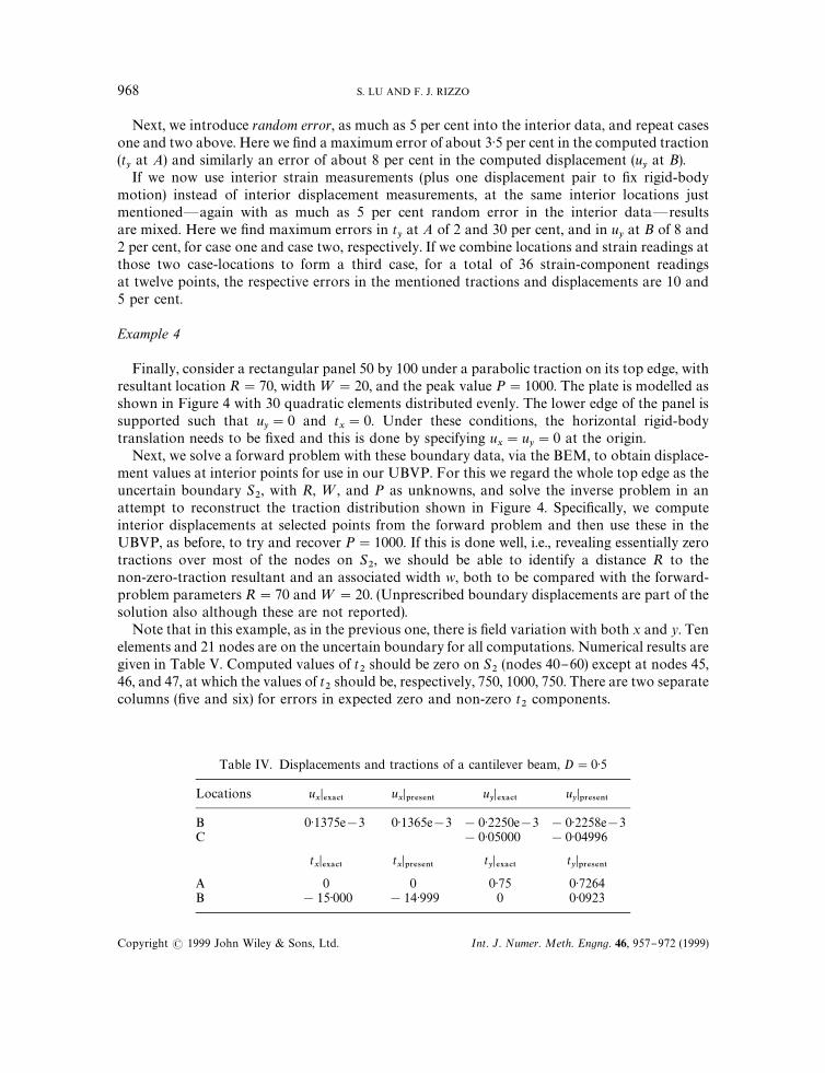
Table IV. Displacements and tractions of a cantilever beam, D"0)5

Locations uxD%9!#5

uxD13%4%/5

uyD%9!#5

uyD13%4%/5

B 0)1375e!3 0)1365e!3 !0)2250e!3 !0)2258e!3C !0)05000 !0)04996

txD%9!#5

txD13%4%/5

tyD%9!#5

tyD13%4%/5

A 0 0 0)75 0)7264B !15)000 !14)999 0 0)0923

Next, we introduce random error, as much as 5 per cent into the interior data, and repeat casesone and two above. Here we "nd a maximum error of about 3)5 per cent in the computed traction(tyat A) and similarly an error of about 8 per cent in the computed displacement (u

yat B).

If we now use interior strain measurements (plus one displacement pair to "x rigid-bodymotion) instead of interior displacement measurements, at the same interior locations justmentioned*again with as much as 5 per cent random error in the interior data*resultsare mixed. Here we "nd maximum errors in t

yat A of 2 and 30 per cent, and in u

yat B of 8 and

2 per cent, for case one and case two, respectively. If we combine locations and strain readings atthose two case-locations to form a third case, for a total of 36 strain-component readingsat twelve points, the respective errors in the mentioned tractions and displacements are 10 and5 per cent.

Example 4

Finally, consider a rectangular panel 50 by 100 under a parabolic traction on its top edge, withresultant location R"70, width="20, and the peak value P"1000. The plate is modelled asshown in Figure 4 with 30 quadratic elements distributed evenly. The lower edge of the panel issupported such that u

y"0 and t

x"0. Under these conditions, the horizontal rigid-body

translation needs to be "xed and this is done by specifying ux"u

y"0 at the origin.

Next, we solve a forward problem with these boundary data, via the BEM, to obtain displace-ment values at interior points for use in our UBVP. For this we regard the whole top edge as theuncertain boundary S

2, with R, =, and P as unknowns, and solve the inverse problem in an

attempt to reconstruct the traction distribution shown in Figure 4. Speci"cally, we computeinterior displacements at selected points from the forward problem and then use these in theUBVP, as before, to try and recover P"1000. If this is done well, i.e., revealing essentially zerotractions over most of the nodes on S

2, we should be able to identify a distance R to the

non-zero-traction resultant and an associated width w, both to be compared with the forward-problem parameters R"70 and="20. (Unprescribed boundary displacements are part of thesolution also although these are not reported).

Note that in this example, as in the previous one, there is "eld variation with both x and y. Tenelements and 21 nodes are on the uncertain boundary for all computations. Numerical results aregiven in Table V. Computed values of t

2should be zero on S

2(nodes 40}60) except at nodes 45,

46, and 47, at which the values of t2should be, respectively, 750, 1000, 750. There are two separate

columns ("ve and six) for errors in expected zero and non-zero t2

components.



Table V. Maximum errors of tractions on uncertain boundary

CaseNo. NMU D/LE

Conditionnumber (A*

22)

Max. [Err (t2)/P]*100%

Zero t2

valuesMax. [Err(t

2)/P]*100%

Non-zero t2

values

1 21 0)05 0)18e9 63 0)12 21 0)10 1)77e9 3583 3)23 21 0)25 1)03e9 307 0)34 21 0)50 2)80e9 73 0)2

5 42 0)10 and 0)50 22,612 0)002 0)0026 42 0)50 and 0)25 18,198 0)0015 0)00027 42 0)05 and 0)25 11,666 0)006 0)002

8 22 0)05 and 0)25 158,000 0)13 0)0049 26 0)05 and 0)25 67,456 0)04 0)002

10 63 0)05, 0)10 and 0)25 11081 38 1311 63 0)05, 0)25 and 0)50 5197 13)9 7)8

Figure 4. BEM model of a rectangular panel under a parabolic traction

Note that for data at 21 interior points on a line parallel to the uncertain boundary, with twodisplacement components at each location, the recovered tractions are not as good as one wouldlike (see cases 1}4 in Table V). This is because the displacement "eld has enough two-dimensionalvariation, such that &one horizontal line of interior data' is simply not enough, no matter howclose the distances D/LE are to the uncertain boundary. When the number of interior points isdoubled to 42, and the interior points are placed on two lines parallel to the uncertain boundary,with di!erent distances D/LE, very good results, with the maximum errors being less than 0)006are obtained (see cases 5}7). One can even get good results by using about half of the points ontwo lines (see cases 8 and 9).



Next, consider cases where there is 3 per cent error, randomly distributed, in the interiordisplacement data. Here we use three rows of interior data points at spacings given in columnthree of cases 10 and 11 in Table V. Errors in computed values of t

2are as indicated in columns

"ve and six. However, without a third row of points, no meaningful solution is even possible witherror in the interior data. Indeed, with the three rows arranged as in case 11*with enough spreadin the rows to pick up the signi"cant y variation in the "eld*results with 3 per cent interior errorare quite respectable for this di$cult problem.

The present example was also chosen in [5] as a test problem. There, 25 iterations of anoptimization computation were needed to obtain results with various (small) errors in the value ofP depending on associated errors in input values of two stress components (in x and y directions)which are provided at thirty nine interior points.

CONCLUDING REMARKS

When faced with a real UBVP, physical measurements of displacement and/or strain, in theinterior of the elastic body, are usually part of the chosen numerical simulation and solutionstrategy. Then these measurements, their locations and the accuracy of their values, are the keyingredients in the solution. From St. Venant's principle we know that su$ciently far (and in mostcases not very far) from a boundary, the di!erences in the interior "elds, associated with di!erentstatically equivalent traction distributions on that boundary, are very di$cult to distinguish.Thus it is clear at the outset that measured information close to an &uncertain boundary' S

2is

more de"nitive of the unknown traction on S2

than that farther away*understanding of coursethat some information su$ciently far from S

2is often required to reveal "eld variation with the

direction normal to S2. Our numerical experiments above support this (cf. Example 4). Of course,

in some cases there may be experimental limitations on how close to S2

one may physically makemeasurements (e.g. locate gages).

Clearly then it is desirable to determine in advance, if possible, where a given number ofavailable gages or other measurements might be located for maximum e!ectiveness*modulo anyexperimental limitations. This assumes, of course, that such measurements must often be limitedin number and that it is desirable to use as few sets of readings (sets of gage locations) as possibleto recover unknown traction distributions on S

2, via the chosen numerical simulation. If all of this

is true, then the strategy o!ered in this paper, which gives "rst a condition number for A*22

basedon gage number, type, and location, for a given discretization of S, can be very valuable to anyUBVP strategy, not only our own. This is because of the intrinsic information about the quality ofthe information about gage location that is inherent in that condition number. (Note, the gagereading itself, however accurate, has no bearing on the condition number). Very generally, what isat work in this step is the richness of the BIE/BEM to relate boundary and interior datain elastostatics in an informative and useful fashion under di$cult theoretical conditions(St. Venant's Principle) and demanding numerical ones. This richness, which is quanti"ed in thecondition number, can be exploited then for any useful purpose.

Now, if one is willing to take another step, namely, choose one or more gage-location-patternswhich are promising, based on the size of the condition numbers for A*

22, one may proceed as

follows. Select one (or perhaps several) "ctitious traction distribution(s) on S2; calculate (via the

forward-problem BEM) the interior displacements and/or strains at the promising locations.Next, perturb these interior values by an amount commensurate with the rated measurement



BOne of our numerical experiments (not reported above) involves reorienting the discretized plate of Example 4 such thatthe smaller dimension 50 at the top now carries the load, with the bottom supported on &rollers' as before. Thus withS2/S"1/6, rather than 1/3 as before, for NMU"18 in two horizontal rows of 9 at D/LE"0)05 and 0)25, the CN

becomes 6209, which is about half the value 11 666 of Case 7 in Table V

accuracy in your gages. Then, with this perturbed data, try to recover the arti"cial tractions, viathe rest of the process outlined above, which uses the SVD for accuracy and the Green's functionlibrary for speed and convenience, and determine the accuracy with which you can recover thesetractions. If desired, one may easily alter a promising pattern and try again. When satis"ed withgage locations and accuracy which might be expected in real recovered tractions based on thosegage locations, one can actually locate the physical gages, take real readings, use the entireprocess illustrated in this paper, and obtain the "nal result for a real UBVP.

Incidentally, if one expects considerable error (beyond the average say) in a few gage readings,using some more gages (if possible) may help the situation. Everything else being equal, morereadings improves a condition number and the detrimental e!ect of isolated errors in any gagereading tends to be reduced.

In general, the Green's function library enables an analyst acquainted with elasticity theory,but perhaps unskilled in sophisticated optimization or minimization processes usually involvedin inverse problems, to quickly and easily do &what-if ' experiments. All may be accomplished witha convenient &point and click' graphical user interface, currently under development, for makingdiscretizations and data entries. If nothing else, we submit that the process described twoparagraphs above could be used as a check, i.e., used to develop con"dence in the solution ofa real UBVP, which might be obtained independently by some other means.

Regarding further research, there is the question about whether displacement or strain data arebetter for the interior measurements needed above. Clearly, our limited experiments are hardlyde"nitive on this matter. We do, however, regard strain as &higher-order' information thandisplacement, and strain varies less with location than displacement does, in many problems*and strain is, of course, independent of rigid-body motion. It would be instructive to test theseobservations quantitatively for bearing on our UBVP solution strategy. Also, the SVD methodo-logy puts error bounds on the solution vector, via the condition number, more precisely than wehave indicated above. Indeed, these bounds involve the largest singular values p

.!9of the matrix

A*22

, as well as the condition number; p.!9

is calculated and printed long with the condition numberitself, during the SVD solution process. Details on this issue of error bounds may be found in [13].

Finally, it is interesting to the authors that in forward problems with BEM, more elements arealmost always better than fewer elements, everything else being equal. But with the inverseproblem solution proposed here, the fewer the number of elements on the uncertain boundaryS2

the better for conditioning of the system of equations which govern a solution. Indeed, thefewer the nodes on S

2the more sharply constrained (in the sense of Hadamard [11]) is the

required distribution of traction on S2. This is good for picking out the desired solution among

the many statically equivalent ones which St. Venant says are present on S2

in the continuous(non-discretized) model, for a "nite number of su$ciently distant interior data points.B The downside of fewer nodes, of course, is a less-accurate representation of the desired solution over S

2.

Such tradeo!s are inherent in the inverse problem itself, though. Every assumption of a solutionform, in terms of a limited number of parameters (cf. 5, 8) provides an essential constraint on thesolution. One distinguishing feature of the present strategy is that all constraints come from thediscretization only. Another feature, the most important one perhaps, is that there is guidance on



how to place displacement and/or strain measurement devices since the present strategy providesa quantitative measure of the conditioning associated with a particular set of internal measure-ment locations.

ACKNOWLEDGEMENTS

This project has been supported in part by the Materials Reliability Division of the NationalInstitute of Standards and Technology (NIST) in Boulder, Colorado under contract No.50RANB70C022 and by the Center for Theoretical and Computational Materials Science(CTCMS) in Gaithersburg, Maryland under grant No. 60NANB6D0210. Also, the authors aregrateful for valuable conversations on UBVPs of the present type with Ambar Mitra, RobertRowlands, Paul Martin and John Berger.

REFERENCES

1. Kubo S. Inverse problems in fracture mechanics. In Computation and Experimental Fracture Mechanics, NisitaniH. (ed.). Computational Mechanics Publications: Southampton, UK, 1994; 139}163.

2. Ingham DB, Yuan Y. BEM for Solving Improperly Posed Problems. Computational Mechanics Publications:Southampton, 1994; 32}34.

3. Zhang F, Kassab AJ, Nicholson DW. A boundary element inverse approach for determining residual stress andcontact pressure. In Boundary Elements, vol. XVII. Computational Mechanics Publications: Southampton, 1995;331}338.

4. Zabaras N, Morellas V, Schnur D. Spatially regularized solution of inverse elasticity problems using the BEM.Communications in Applied Numerical Methods 1987; 5:547}553.

5. Mezerra LM, Saigal S. Inverse boundary traction reconstruction with the BEM. International Journal of Solids andStructures 1995; 32:1417}1431.

6. Berger JR, Tewary VK. Boundary element analysis of moire "elds in anisotropic materials. Engineering Analysis withBoundary Elements 1996; 18:17}325.

7. Das S. Numerical Solution of Inverse Problems in Mechanics using the BEM. Ph.D. Dissertation, ISU, 72}73, 1991.8. Schnur DS, Zabaras N. Finite element solution of 2-D inverse elastic problems using spatial smoothing. International

Journal for Numerical Methods in Engineering 1990; 30:57}75.9. Rizzo FJ. An integral equation approach to boundary value problems of classical elastostatics. Quarterly Applied

Mathematics 1967; 25:83}95.10. Hartmann F. Introduction to Boundary Element, ¹heory and Applications. Springer: Berlin, Heidelberg, 1989.11. Hadamard J. ¸ectures on the Cauchy Problem in ¸inear Partial Di+erential Equations. Yale University Press:

New Haven, 1923.12. Timoshenko S, Goodier JN. ¹heory of Elasticity (2nd edn). McGraw-Hill: New York, 1951; 51.13. Forsythe GE et al. Computer Methods for Mathematical Computations. Prentice-Hall: New Jersey, 1977; 192}239.14. Pan L, Adams DO, Rizzo FJ. BEM analysis for composite materials and a library of Green's functions. Computers and

Structures 1997; 6(5):685}693.15. Lu S, Rizzo FJ. Partitioning with BEM: discretized Green's function libraries for elastodynamics and acoustics.

In Proceedings of International Conference on Computational Engineering Science +98, 1998.16. Banerjee PK. ¹he Boundary Element Methods in Engineering. Mc-Graw-Hill: London, 1994.17. Kane JH, Keyes DE, Prasad KG. Iterative solution techniques in boundary element analysis. International Journal for

Numerical Methods in Engineering 1991; 31:1511}1536.18. Kane JH. Boundary Element Analysis in Engineering Continuum Mechanics. Prentice-Hall: New Jersey, 1994.19. Golub GH, Van Loan CF. Matrix Computations. 2nd edn, Johns Hopkins University Press: Baltimore, 1989.20. Fiedler M. Special Matrices and their Applications in Numerical Mathematics. Martinus Nijho!: Dordrecht, 1986.21. Przemieniecki JS. ¹heory of Matrix Structural Analysis. McGraw-Hill: New York, 1968.22. Hsiao GC, Wendland WL. Domain decomposition in boundary element methods. In Fourth International Symposium

on Domain Decomposition Methods for Partial Di+erential Equations, Glowinski R et al. (eds). SIAM: Philadelphia,1991; 41}49.

23. Hsiao GC, Wendland WL. Domain decomposition via boundary element methods. In Numerical Methods inEngineering and Applied Sciences, Alder H et al. (eds). CIMNE: Barcelona, 1992; 198}207.

24. Martin PA, Rizzo FJ. Partitioning, boundary integral equations, and exact Green's functions. International Journalfor Numerical Methods in Engineering 1995; 38:3483}3495.



A boundary element strategy for elastostatic inverse problems involving uncertain boundary...

Documents

Transcript of A boundary element strategy for elastostatic inverse problems involving uncertain boundary...