Theory of the polarization of highly-charged ions in Theory of the polarization of highly-charged ions in storage rings: production, preservation and application storage rings: production, preservation and application

to the search for the violation of the fundamental to the search for the violation of the fundamental symmetriessymmetries

A. BondarevskaA. Bondarevskayyaa

A. Prozorov A. Prozorov

L. LabzowskyL. Labzowsky,, St. Petersburg State University, Russia

D. Liesen D. Liesen

F. Bosch F. Bosch GSI Darmstadt, Germany

G. Plunien G. Plunien Technical University of Dresden, Germany

St.-Petersburg, 2010

1. Production of polarized HCI beams1. Production of polarized HCI beams 1.1 Radiative polarization: simple estimates

Radiative polarization occurs via radiative transitionsRadiative polarization occurs via radiative transitions

between Zeeman sublevels in a magnetic fieldbetween Zeeman sublevels in a magnetic field

first discussed in: A.A. Sokolov, I.M. Ternov, Sov. Phys.Dokl. 8 (1964) 1203

first realized in Novosibirsk for electrons: Ya.S. Derbenev, A.M. Kondratenko, S.T. Serednyakov, A.N. Skrinsky,

G.M. Tumaikin, Ya.M. Shatunov, Particle accelerators 8 (1978) 115

recent development:S.R. Mane, Ya.M. Shatunov and K. Yokoya J.Phys.G 31 (2005) R151;

Rep. Progr. Phys. 68 (2005) 1997

Spin-flip transition rates for electrons (lab.system)

W W spin-flipspin-flip = 64 (3 = 64 (3 ћћcc33))-1-1 │ │μμ00││55 H H33 γγ55

γγ = Lorentz factor; H = magnetic field, = Lorentz factor; H = magnetic field, μμ00 = Bohr magneton = Bohr magneton

Polarization time Polarization time TTPP = W = W -1-1

Electrons: H ≈ 1 T, γ ≈ 10 5, TP ≈ 1 hour

Protons: μ << μ0 →TP huge

HCI: μ ≈ μ0, but even for FAIR at GSI with H ≈ 6 T, γ ≈ 23 → TP ≈ 103 hours → too long !

1.2 Selective laser excitation of the HFS levels* 1.2 Selective laser excitation of the HFS levels*

Schematic picture of the Schematic picture of the Zeeman splitting of the Zeeman splitting of the

hyperfine sublevels of the hyperfine sublevels of the electronic ground state for the electronic ground state for the

H-like 151Eu ion (I = 5/2). (I = 5/2).

gJ - electron g-factor.

* A. Prozorov, L. Labzowsky, D. Liesen

and F. Bosch

Phys. Lett. B574 (2003) 180

The solid lines denote M1 excitationsat a laser frequency ω = ΔEHFS + 2 μ0H.

ΔEHFS = 1.513 (4) eV.

The dashed lines show the decay channels for Zeeman sublevels.

1s1/2

1s1/2

F = 2

F' = 3

MF'

MF

,μ1)2F(F

1)I(I-1)J(J1)F(FgE 0J

FZee

Transition rate Transition rate

W (F'=3 → F=2) = 0.197· 102 s-1

W (F' MF' → FMF) = const [CFF'1, MF-MF' (MF, MF')]2 ,

CFF'1, MF-MF' (MF, MF') are Clebsh-Gordan coefficients

The selective laser excitation to the 1sThe selective laser excitation to the 1s1/21/2 F' = 3 state is F' = 3 state is

performed by a laser with frequency performed by a laser with frequency ω. This leads to the . This leads to the partial polarization of the 1s of the 1s1/21/2 F' = 3 state. F' = 3 state.

After the laser is switched off, the spontaneous decay to After the laser is switched off, the spontaneous decay to the ground state leads to its partial polarization during the ground state leads to its partial polarization during

10.9 ms (lifetime of the F' = 3 level).(lifetime of the F' = 3 level).

1.3 Description of polarization

The polarization state of an ion after i-th "cycle"The polarization state of an ion after i-th "cycle"

(switching on the laser) is described by the density matrix:(switching on the laser) is described by the density matrix:

ρF(i) = ΣMF nFMF

(i) ψFMF* ψFMF .

Normalization condition: Normalization condition: ΣΣMFMF n nFMFFMF(i)(i) = 1, = 1,

ψFMF are the wavefunctions, nFMF(i) the occupation numbers

F, MF the total angular momentum and projection of an ion

Degree λ of polarization is defined as:

λF (i) = F-1 ΣMF nFMF(i) MF

Nonpolarized ions: nFMF = (2F + 1) -1, λF = 0

Fully polarized ions: nFF = 1, λF = 1

1.4 Dynamics of polarization

The occupation numbers are defined with the recurrence relations The occupation numbers are defined with the recurrence relations via the M1 transition probabilities:via the M1 transition probabilities:

width of the sublevel F’M’width of the sublevel F’M’FF

FFFF MM'1)-(i

FM(i)

M'F' δn2

1n

)1-i(FM

(i)M'F'

1M,MM' F

FF(i)FM FF

FFF

Fn

2

1n

)M'(F'

)FMM'W(F'

2

1n

FM

FFF )FMM'W(F')M'F'(

Opposite initial populationOpposite initial population

λλ FF(0)(0) = -1, n = -1, n F-FF-F

(0)(0) = 1 = 1

After first cycle: After first cycle: λλ FF(1)(1) = - 0.6667 = - 0.6667

After 40 cycles: After 40 cycles: λλ FF(40) (40) = 0.9986= 0.9986

The polarization time for

λF(40) = 0.999

TP = 40 · 10.9 ms = 0.44 s

40

1

010

λ+2

+10

Uniform initial population Uniform initial population λλ F

(0)(0) = 0, n = 0, n FMF(0)(0) = (2F+1) = (2F+1)-1-1

After After first cycle: cycle: λλ F(1)(1) = = 0.1667

After After 40 40 cycles: λλ F(40)(40) = = 0.9993

λ, nFMF

N

1.5 1.5 Nuclear polarization polarization Nuclear polarization density matrix

ρρII = < = < ψψFMFFMF │ │ρρFF│ψ│ψFMFFMF > >elel (integration over electron variables) (integration over electron variables)

ψFMF = ΣMIMJ CFMF IJ (MIMJ) ψIMI ψJMJ ψIMI , ψJMJ nuclear, electronic wave functions

ρρII = = ΣΣMIMI n nIMIIMI ψψIMIIMI* * ψψIMI IMI ; n; nIMIIMI = = ΣΣMJMFMJMF n nFMFFMF [C [CFMFFMF (M (MIIMMJJ)])]22

Degree Degree λλ of nuclear polarization: of nuclear polarization:

λλI I = I= I-1-1 ΣΣMIMI n nIMI IMI MMII

Maximum nuclear polarization for the case of full electron Maximum nuclear polarization for the case of full electron polarization nFF = 1 (F = 2) in Eu ions: λI

max = 0.93

1.6 Polarization of one- and two-electron ions of one- and two-electron ions

Polarization in He-like ions with total electron angular momentumequal to zero (2 1S0, 2 3P0) is nuclear polarization.

In polarized In polarized one-electron HCI the nuclei are also polarized, the nuclei are also polarized,due to the strong hyperfine interaction (hyperfine splitting due to the strong hyperfine interaction (hyperfine splitting in the order of in the order of 1 eV). Polarization time is about ). Polarization time is about 10 -15 s. .

The capture of the second electron by the polarized one-electronion does not destroy the nuclear polarization: the capture time,defined by the Coulomb interaction, is much smaller than the depolarization time, defined by the hyperfine interaction. If thetotal angular momentum of the two-electron ion appears to be

zero (2 1S0, 2 3P0) the nuclear polarization remains unchanged.

2. Preservation of the ion beam polarization in storage rings

2.1 Dynamics of the HCI in a magnetic system of a storage ring

The magnetic system of a storage ring (GSI) consists of a number of The magnetic system of a storage ring (GSI) consists of a number of magnets including magnets including bending magnets which generate field magnets which generate field

components components orthogonal to the ion trajectory, to the ion trajectory, focusing quadrupole quadrupole magnets and the magnets and the longitudinal electron cooler magnet (solenoid). electron cooler magnet (solenoid).

The latter one was also proposed to be used for the The latter one was also proposed to be used for the longitudinal polarization of the ions via selective laser excitation. of the ions via selective laser excitation.

The peculiarity of storing polarized HCI compared to stored electrons The peculiarity of storing polarized HCI compared to stored electrons or protons is that theor protons is that the trajectory dynamics is defined by the is defined by the

nuclear mass, whereas thewhereas the spin dynamics is defined by the is defined by the electron mass..

The The movement of an ion in a magnetic system of a ring can in a magnetic system of a ring can

be described be described classically with the equation of motion: with the equation of motion:

dv/dt = k (H x v)

k = -Ze/Mc, v is the ion velocity, M, Ze are mass and charge of

the nucleus, H is the magnetic field

In the rest frame of an ion the motion appears like in a time-dependent field.

The spin dynamics which is influenced by the transitions between hyperfine and Zeeman sublevels we describe quantum -

mechanically.

2.2 Spin dynamics and the instantaneous quantization axis (IQA)

Relativistic effects are neglected (at GSI ring Relativistic effects are neglected (at GSI ring γγ ≈≈ 1) 1)

Spin motion in the ion reference system is described by the Spin motion in the ion reference system is described by the Schrödinger equation:Schrödinger equation:

[i ∂/∂t + μ0H(t) s] χS(t) = 0 (∗)

H(t) is the magnetic field, s is the spin operator

The IQA, denoted as ζ, we define via an equation:

∂/∂t < χS(t)│s ζ(t)│χS(t) > = 0 (∗∗)

From (∗) and (∗∗) follows the equation for IQA:

∂ζ/∂t = μ0 (H(t) x ζ(t)) (∗∗∗)

Equation (Equation (∗∗∗∗∗∗) coincides with the ) coincides with the pure classical equation for for the spin motion, however the definition (the spin motion, however the definition (∗∗∗∗) is convenient ) is convenient

for the quantum-mechanical description of polarization.for the quantum-mechanical description of polarization.

It can be proved that the It can be proved that the degree of polarization with respect to with respect to IQA remains IQA remains constant in an arbitrary time-dependent field. in an arbitrary time-dependent field.

It can be also proved that the It can be also proved that the degree of polarization with with respect to IQA respect to IQA does not change in the process of in the process of

spontaneous decay of the excited hyperfine sublevel, i.e. of the excited hyperfine sublevel, i.e. remains the same for the ground- and excited hyperfine remains the same for the ground- and excited hyperfine

sublevels.sublevels.

2.3 Rotation of IQA in the magnetic field of a bending magnet at GSI ring

The initial polarization is directed along the longitudinal (z) axis:The initial polarization is directed along the longitudinal (z) axis:

ζx(0) = 0, ζy(0) = 0, ζz(0) = 1

The magnetic field The magnetic field H is oriented along the vertical (x) axis: is oriented along the vertical (x) axis:

Hx = H(t), Hy = Hz = 0

Solution of the Schrödinger equation reads:Solution of the Schrödinger equation reads:

ζζxx(t) = 0, (t) = 0, ζζyy(t) = sin (t) = sin φφ(t), (t), ζζzz(t) = cos (t) = cos φφ(t)(t)

tt

φ(t) = μ0/ћ ∫ H(t') dt' (A) 0

The IQA rotates in the horizontal plane (yz) with the time-dependent frequency ω(t) = φ(t) / t

The trajectory rotation occurs due to the Lorentz force. Roughly we can write the rotation angle for the ion trajectory after passing one

GSI bending magnet (600 = π/3):

t

μN/ћ ∫ H(t') dt' = π/3 (B) 0

where μN = Zmμ0/M. For Eu ions μN = 2.268 · 10 -4 μ0

By comparing eqs. (A) and (B) we conclude that the rotation angle for IQA after passing one bending magnet amounts to about 104 π. Thus, it will be extremely difficult to fix the direction of polarization before the start of the PNC experiment.

2.4 Solution of the problem: "Siberian Snake" AA Siberian Snake Siberian Snake rotates the polarization (IQA) the polarization (IQA) by an angle π around the z-axis. If after one revolution of an ion in the ring the . If after one revolution of an ion in the ring the IQA will acquire a deviation from the longitudinal direction, the IQA will acquire a deviation from the longitudinal direction, the

Siberian Snake will rotate it like:Siberian Snake will rotate it like:

beam

SiberianSiberian SnakeSnake

IQA

IQA

Then, after two revolutions, the deviation caused by any reasonwill be canceled. It remains to count the revolutions and to start a PNC experiment after an even number of revolutions.Counting

the revolutions seems to be possible for a bunched beam.

3. Diagnostics of polarization3.1 TheThe hyperfine quenchinghyperfine quenching (HFQ) of polarized two- electron ions in an external magnetic field

The HFQ transition probability for the polarized ion in an external The HFQ transition probability for the polarized ion in an external magnetic field:magnetic field:

WWHFQ HFQ = W = W00HFQHFQ [ 1 + Q [ 1 + Q11((ζhζh)])]

where Wwhere W00 HFQ HFQ is the HFQ transition rate in the absence of the external is the HFQ transition rate in the absence of the external

field, field, and and hh==HH//||HH|.|.In case of the 2 In case of the 2 11SS00 – 1 – 1 11SS00 HFQ, the coefficient Q HFQ, the coefficient Q11 is: is:

Q11 = 2 λ < 2 1S0 │μH│2 3S1 > / < 2 1S0 │HHF│2 3S1 >

μ is the magnetic moment of an electron, HHF is the hyperfine interaction Hamiltonian

The net signal (after switching off the magnetic field) is:

Δ WHFQ = Q1 W0HFQ

too small to be observed!

However, as we shall see this is the unique experiment which However, as we shall see this is the unique experiment which allows for the allows for the direct direct measurement of the degree of polarization measurement of the degree of polarization 𝜆 𝜆 in the HFQ transitionin the HFQ transition

For He-like Eu (Z = 63) and H = 1 T→ Q1 = -10-7

3.2 Employment of Employment of RECREC (Radiative Electron Capture) (Radiative Electron Capture)

Employment of REC for the control of polarization of HCI beams via measurement of linear polarization of X-rays was

studied in:

A. Shurzhikov, S. Fritzsche, Th. Stöhlkerand S. Tashenov,

Phys. Rev. Lett. 94 (2005) 203202

The formula tan 2χ ~ λ F was confirmed experimentally (for λ F = 0) by:

S. Tashenov et al. PRL 97 (2006) 223202

We will study the possibility for the control of the HCI beam We will study the possibility for the control of the HCI beam polarization via measurement of linear polarization of X-rays polarization via measurement of linear polarization of X-rays

in HFQ transitions.in HFQ transitions.

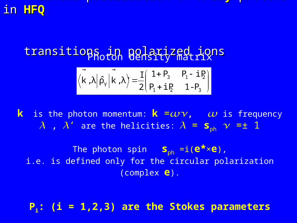
3.3 Linear polarization of Linear polarization of X-rayX-ray photons in photons in HFQHFQ transitions in polarized ions transitions in polarized ions

Photon density matrix

k is the photon momentum: k =𝜔𝜈, 𝜔 is frequency𝜆 , 𝜆‘ are the helicities: 𝜆 = sph 𝜈 =± 1The photon spin sph =i(e*×e),

i.e. is defined only for the circular polarization (complex e).

Pi: (i = 1,2,3) are the Stokes parameters

321

213γ P - 1iPP

iPPP 1

2

I λ' , k ρ λ , k

3.4 Stokes parameters

900

9001 II

IIP

13545

135452 II

IIP

P3 - circular polarization

Iα – intensity of the light, polarized along

the axis α.Stokes parameters via photon density

matrix:

1kρ1k1kρ1k

1kρ1k1kρ1kP

γγ

γγ

1

1kρ1k1kρ1k

1kρ1k1kρ1kiP

γγ

γγ

2

Schematic position of the axes in the X-ray polarization observation

experiment

3.5 Rotation of the photon density matrix of the photon density matrix

Choice of the quantization axis: along IQAIQA (beam polarization).

The photon density matrix is written with the quantization axis ν. It is necessarynecessary to rotate this matrix by an angle 𝜃.The result for the transition between two bound states with the total electron momentum j, j‘

Here: A𝜆 LML - photon wave function, LML – photon angular momentum and projection, 𝛼 – Dirac matrices njm – occupation numbers for the initial electron states (define electron polarization)D𝜈0𝜇(𝜃) – Wigner function; in our case 𝜃=450

jmLL'

m'mL-L

MLLMmm'νμ

ν0μγ n1)(i(θθDConstj',λ,kρjλ,,k

LL

*λLM

λ''ML'

LLνμLL

LLν0 m'j'Aαjmm'j'Aαjm)λλ(C)M'M(C

LL

3.6 Application to the 2211SS00→1→111SS00 HFQ transition (magnetic dipole photons)FF – total angular momentum of an ion; nFMF

– occupation numbers

Nonplarized ions: nFMF = const: PPMM

11=0=0;

PPMM22=0=0 independent on the polarization.

Hence, the photons are nonpolarized if they are emitted by nonpolarized by

nonpolarized ions.

For 2211SS00 state of 1511516363EuEu61+ 61+ : F=I=5/2, n5/2 5/2 = 5/6, n5/2 3/2 = 1/6

𝜆 F = 𝜆I = (1/F) ΣMF nFMF

MF = 0.93

PPMM11 = -0.4= -0.4, PPMM

22=0=0

3)1)(2F1)F(F(2F

1)F(F3MnConstP

2F

MFM

M1

F

F

3.7 Polarization and Polarization and alignment

Thus, one cannot extract the degree of polarization 𝜆F from the Stokes parameters

Stokes parameter PM1 defines „the degree of alignmentthe degree of alignment“ which can be

defined as

aaFF = =ΣΣMMFF n nFMFMFF

M MFF22

- a - a00FF

where a0F =ΣMF

(2F+1)-1 MF2

= 1/3 F(F+1)

Then for the fully nonpolarized ions aF=0.

However, using the value of aF (as extracted from PM1) one can check

whether the ion polarization has its maximum value.

For the maximum polarization nFMF = 𝛿 F,MF and

aamaxmaxFF = 1/3 F(2F - 1) = 1/3 F(2F - 1)

3.8 Stokes parameters for the parameters for the 2233PP00→1→111SS0 0 HFQ HFQ

transition (electric dipole photons)transition (electric dipole photons)

For the investigation of the PNC effects in He-like Eu and Gd ions it will be important to know also the Stokes parameters for electric photons

(transition 2233PP00→1→111SS0 0 ).

For Eu ions: PPEE11 = + 0.4= + 0.4, PPEE

22=0=0

The result PPM,EM,E11 = = ∓∓ 0.4 0.4 means that 70% of ions, polarized along I0 axis

are electric ones, and 70% of ions, polarized along I90 axis are magnetic

ones.

3.9 Impossibility to measure the degree of the ion to measure the degree of the ion polarization via linear polarization via linear X-ray polarizationpolarization..

There are general arguments why the beam polarization (i.e. the degree of polarization) cannot be defined via the linear polarization of emitted

photons.

If it would be possible, the probability should contain a pseudeoscalarpseudeoscalar

term, constructed from the vectors 𝜻 and e (for electric photons) or 𝜻 and (e ×k) (for magnetic ones). Moreover, this term should be quadratic

in e or (e ×k). It is easy to check that such constructions, linear in 𝜻, cannot be built, and only quadratic in 𝜻 terms like (𝜻e)2 or (𝜻(e×k))2 can arise. From these quadratic terms one can define the alignment, but

not the polarization.The only possibility to measure the beam polarization via X-ray

polarization is to use the circular polarization. Then

WHFQ = WHFQ0 [1 + Q2 (𝜻 sph)]

sph = i (e*×e) photon spin

44. PARITY NONCONSERVATION EFFECTS IN . PARITY NONCONSERVATION EFFECTS IN HCI

4.1 POSSIBLE PARITY NONCONSERVATION (PNC) EFFECTS IN ONE-PHOTON TRANSITIONS FOR ATOMS AND IONS

WWifif = W = Wifif00 [ 1 + ( [ 1 + (ssphphnn)R)R11 + ( + (ζn)Rζn)R22 + ( + (hnhn)R)R33

+ (+ (ζhζh)Q)Q11 + ( + (ζsζsphph)Q)Q22 ] ]

nn = direction of photon emission = direction of photon emission

ssphph = photon spin = photon spin

ζζ = direction of ion polarization = direction of ion polarization

hh = direction of external magnetic field (unit vector) = direction of external magnetic field (unit vector)

4.2 Parity 4.2 Parity violating coefficients coefficients

RR11 = Re [ -i < i │HW │a > (Ei - Ea - i Γ/2)-1 (Waf / Wif)1/2 ]

HHWW = effective PNC Hamiltonian = effective PNC Hamiltonian

i,f = initial, final statei,f = initial, final state

a = state admixed to state i by Ha = state admixed to state i by HWW

RR22 = = λλRR11 ((λλ = degree of ion beam polarization) = degree of ion beam polarization)

R3*= Re [(< i│μH│i > + < a│μH│a >) (Ei - Ea - i Γ/2) -1] R1

μ = magnetic moment of the electron; H = external magnetic field* Ya. A. Azimov, A. A. Anselm, A. N. Moskalev and R. M. Ryndin

Zh. Eksp. Teor. Fiz. 67 (1974) 17

4.3 Parity 4.3 Parity conserving coefficients coefficients

QQ1 1 = λ Re [ (< i │μH │i > + < b│μH│b >)

· (Ei - Ea - i Γ/2)-1 (Wbf / Wif)1/2 ]

b = level closest to level i of the same parity, b = level closest to level i of the same parity,

admixed by the magnetic field Hadmixed by the magnetic field H

QQ22 = a = a λλ, a ≈ 1, a ≈ 1

Data from:

A.N. Artemyev, V.M. Shabaev,V.A. Yerokhin, G. Plunien andG. Soff,

Phys.Rev. A71 (2005) 062104

4.4 4.4 He-like HCI: level crossings HCI: level crossings

δ(23P0) = [E(21S0) – E(23P0)] / E(21S0)

δ(23P1) = [E(21S0) – E(23P1)] / E(21S0)

ΔE/E

110Z

δ (2 3P1)

5·10-3

10-3

δ (2 3P0)

δ (2 3P0)

δ (2 3P1)

4.5 4.5 PNC effects in effects in He-like HCI: a survey of proposalsHCI: a survey of proposals

V.G. Gorshkov and L.N. LabzowskyV.G. Gorshkov and L.N. Labzowsky

Zh. Eksp. Teor. Fiz. Pis' ma Zh. Eksp. Teor. Fiz. Pis' ma 1919 (1974) 30 (1974) 30

2211SS00 - 2 - 233PP11 crossing Z = 6, 30, nuclear spin-dependent weak constant, R =10 crossing Z = 6, 30, nuclear spin-dependent weak constant, R =10 -4-4

A. Schäfer, G. Soff, P. Indelicato and W. GreinerA. Schäfer, G. Soff, P. Indelicato and W. Greiner

Phys. Rev Phys. Rev A40A40 (1989) 7362 (1989) 7362

2 2 11SS00 – 2 – 2 33PP00 crossing, Z = 92, two-photon laser excitation crossing, Z = 92, two-photon laser excitation

G. von OppenG. von Oppen

Z. Phys. Z. Phys. D21 (1991) 181 (1991) 181

2 2 11SS00 – 2 – 2 33PP00 crossing, Z = 6, Stark-induced emission, R = 10 crossing, Z = 6, Stark-induced emission, R = 10 -6-6

V.V. Karasiev, L.N. Labzowsky and A.V. Nefiodov V.V. Karasiev, L.N. Labzowsky and A.V. Nefiodov

Phys. Lett. Phys. Lett. A172A172, 62 (1992), 62 (1992)

2 2 11SS00 – 2 – 2 33PP00 crossing in U (Z = 92), HFQ decay R ~ 10 crossing in U (Z = 92), HFQ decay R ~ 10-4-4

R.W. DunfordR.W. Dunford

Phys. Rev. A54 (1996) 3820(1974) 30Phys. Rev. A54 (1996) 3820(1974) 30

2 2 11SS00 – 2 – 2 33PP00 crossing Z = 92, stimulated two-photon emission, R = 3 crossing Z = 92, stimulated two-photon emission, R = 3 ··10 10 -4-4

L.N. Labzowsky, A.V. Nefiodov, G. Plunien, G. Soff, R. Marrus and D. LiesenL.N. Labzowsky, A.V. Nefiodov, G. Plunien, G. Soff, R. Marrus and D. Liesen

Phys. Rev Phys. Rev A63A63 (2001) 054105 (2001) 054105

2211SS00 – 2 – 233PP00 crossing, Z = 63, hyperfine quenching with polarized ions, R = 10 crossing, Z = 63, hyperfine quenching with polarized ions, R = 10 -4-4

A.V. Nefiodov, L.N. Labzowsky, D. Liesen, G. Plunien and G. SoffA.V. Nefiodov, L.N. Labzowsky, D. Liesen, G. Plunien and G. Soff

Phys. Lett. BPhys. Lett. B534 (2002) 52 (2002) 52

2211SS00 – 2 – 233PP11 crossing, Z = 33, nuclear anapole moment, polar. ions, R = 0.6 crossing, Z = 33, nuclear anapole moment, polar. ions, R = 0.6··10 10 -4-4

G.F. Gribakin, E.F. Currell, M.G. Kozlov and A.I. MikhailovG.F. Gribakin, E.F. Currell, M.G. Kozlov and A.I. Mikhailov

Phys. Rev. Phys. Rev. A72A72, 032109 (2005), 032109 (2005)

2 2 11SS00 – 2 – 2 33PP00 crossing Z = 30 – Z = 48, crossing Z = 30 – Z = 48, dielectronic recombinationdielectronic recombination, polarized , polarized

incident electrons, R ~ 10incident electrons, R ~ 10-8-8

A.V. Maiorova, O.I. Pavlova, V.M. Shabaev, C. Kozhuharov, A.V. Maiorova, O.I. Pavlova, V.M. Shabaev, C. Kozhuharov,

G. Plunien and Th. StoelkerG. Plunien and Th. Stoelker

J. Phys. B J. Phys. B 4242 205002 (2009) 205002 (2009)

2 2 11SS00 – 2 – 2 33PP00 crossing, Z = 90, 64 radiative recombination crossing, Z = 90, 64 radiative recombination

linear X-ray polarizationlinear X-ray polarization, polarized electrons, R ~ 10 , polarized electrons, R ~ 10 -8-8

4.6 Energy Level Scheme for 4.6 Energy Level Scheme for He-like Gd

Numbers on the r. h. side:ionization energies in eV

The partial probabilities ofthe radiative transitions: s-1

Numbers in parentheses:powers of 10

Double lines: two-photon transitions

I, g I :nuclear spin, g-factor

157Gd : I =3/2, g I = - 0.3398

4.7 Energy Level Scheme for 4.7 Energy Level Scheme for He-like Eu

Numbers on the r. h. side:ionization energies in eV

The partial probabilities ofthe radiative transitions: s-1

Numbers in parentheses:powers of 10

Double lines: two-photon transitions

I, g I :nuclear spin, g-factor

151Eu : I =5/2, g I = + 3.4717

4.8 4.8 PNC effect in He-like effect in He-like polarized HCI HCI

Basic Basic hyperfine-quenched (HFQ) transition:(HFQ) transition:

││1s2s 1s2s 11SS00 > + > + 11//ΔΔEESS<1s2s <1s2s 11SS00 │ │H hfhf│ 1s2s │ 1s2s 33SS11> > │1s2s │1s2s 33SS11 > >

→ │1s2 1S0 > + γ (M1) where Hhf = hyperfine interaction Hamiltonian, ΔES = [ E(2 3S1) – E(2 1S0) ]

PNCPNC - allowed transition:

││1s2s 1s2s 11SS00 > + > + 11//ΔΔEESPSP<1s2s <1s2s 11SS00 │ │H WW│1s2p │1s2p 33PP00>>

11//ΔΔEEPP<1s2p <1s2p 33PP00 │ │H hfhf│ 1s2p │ 1s2p 33PP11> > · · │1s2p │1s2p 33PP11 > >

→ │1s2 1S0 > + γ (E1)

where ΔESP = [ E(2 3P0) – E(2 1S0) ], ΔEP = [ E(2 3P1) – E(2 3P0) ] ,

R2 = λ [ W HFQ + PNC (E1) / W HFQ (M1)]1/2

4.9 Evaluationt of the 4.9 Evaluationt of the coefficient R2

One-electron One-electron polarized ions: ions:

dWdWjj’ jj’ = dW = dW(0)(0)jj‘ jj‘ + + dWdW(PNC)(PNC)

jj‘ jj‘

dWdW(0)(0)jj‘ jj‘ = = ΣΣλλ <<kk,,λλ,njl,njl │ │ρργγ│ 1s2s │ 1s2s 33SS11> > ││ kk,,λλ,n’j’l’,n’j’l’ >>

Parity Parity nonconservation:

││ njlmnjlm > → │> → │ njlmnjlm > + [ E> + [ En’’jl’’ n’’jl’’ – E– Enjlnjl]]-1-1<njlm│<njlm│H WW│n‘‘jl‘‘m>│n‘‘jl‘‘m> │ │ n’’jl’’mn’’jl’’m > >

H W = - GF/2√2 QWρN(r)γ5 , QW = - N + Z (1 – 4sin2θW),

GF - Fermi constant , ρN(r) – charge density distribution in the nucleus

After rotating the photon quantization axis to the direction of the After rotating the photon quantization axis to the direction of the IQA (ion beam polarization axis) and by an angle IQA (ion beam polarization axis) and by an angle θθ

cos cos θθ = (𝜻 = (𝜻νν))

and after summation over the angular momentum projections and after summation over the angular momentum projections

we obtain the following resultwe obtain the following result

4.10 Basic magnetic dipole transition (l = l‘) for 4.10 Basic magnetic dipole transition (l = l‘) for one-electron ionsone-electron ions

dWdWnjl,n’jl njl,n’jl = dW = dWM1M1njl,n‘jl njl,n‘jl [1 + [1 + RR22 ( (𝜻𝜻νν) ) λλ]]

RR22 = - 2 = - 2ηηnjl,n’’jlqnjl,n’’jlq R RE1E1(n’’jlq ;n’j’l)/ R(n’’jlq ;n’j’l)/ RM1M1(njl;n’j’l), lq = 2j - l(njl;n’j’l), lq = 2j - l

ηnjl,n’’jlq = Gnjl,n‘‘jlq / En’’jlq – Enjl

Gnjl,n‘‘jlq = - (GF/2√2) QW ∫[Pnjl(r)Qn’’jlq(r) – Qnjl(r)Pn’’jlq(r)] ρN(r)r2dr

Pnjl(r), Qnjl(r) – upper and lower radial components of the Dirac wave – upper and lower radial components of the Dirac wave

function for the electronfunction for the electron

RE1, RM1 – reduced matrix elements for the electric and magnetic dipole – reduced matrix elements for the electric and magnetic dipole

transitionstransitions

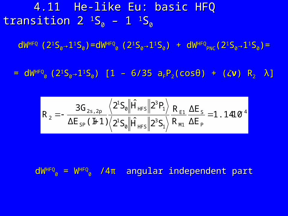
4.11 He-like Eu: basic HFQ transition 2 4.11 He-like Eu: basic HFQ transition 2 11SS00 – 1 – 1 11SS00

dWdWHFQHFQ ((2211SS00→1→111SS00))=dW=dWHFQHFQ

0 0 ((2211SS00→1→111SS00) + ) + dWdWHFQHFQPNCPNC((2211SS00→1→111SS00)=)=

== dW dWHFQHFQ0 0 ((2211SS00→1→111SS00) [1 – 6/35 a) [1 – 6/35 aFFPP22(cos(cosθθ) + () + (𝜻𝜻νν) ) RR22 λλ]]

dWdWHFQHFQ00 = = WWHFQHFQ

0 0 /4 /4ππ angular independent partangular independent part

4

P

S

M1

E1

13

HFS01

13

HFS01

SP

2s,2p2 101.14

ΔE

ΔE

R

R

S2HS2

P2HS2

1)(IΔE

3GR

4.12 Possible determination of the degree of 4.12 Possible determination of the degree of alignment a aFF

The term containing aF gives the possibility to measure the degree of

alignment (or to check whether the maximum polarization is achieved) in a most simple way. This term has no smallness no smallness compared to 1, provided that the polarization (and alignment) is of the order of 1. It is parity conserving parity conserving and corresponds to the scalars of the type (𝜻ν)2, ( ×𝜻 ν)2 in the expression for the probability. It also vanishesvanishes when the polarization is absent, since

then aF = 0.For defining aF one has to measure dWHFQ for two different angles:

dWdWHFQHFQ ( (θθ=0) - =0) - dWdWHFQHFQ ( (θθ==ππ/2) / /2) / dWdWHFQHFQ 00 = - (18/35) = - (18/35) aaFF

4.13 PNC effect in He-like HCI: Gd versus Eu 4.13 PNC effect in He-like HCI: Gd versus Eu

ΔE = E(21S0) – E(23P0) from Artemyev et al. 2005

ΔE (Gd) = + 0.004 ± 0.074 eV Z = 64

ΔE (Eu) = - 0.224 ± 0.069 eV Z = 63Re (ΔE – i Γ/2) -1 = ΔE (ΔE2 + Γ2/4) -1; Γ(Gd) = 0.0016 eV (HFQ E1 23P0→11S0)

Lifetime (s) Lifetime (s) R(max) / λ R(min) / λ Z 2 3P0 (HFQ E1) 2 1S0 (2 E1)

64 4 · 10 -12 1.0 · 10 -12 0.052 (ΔE = Γ) 0 (ΔE = 0)

63 4 · 10 -13 1.2 · 10 -12 1.0 · 10 -4 0.6 · 10 -4

Disadvantage of Gd: Lifetime of 2 3P0 longer than lifetime of 2 1S0

HFQ (E1) transition 2 3P0 → 1 1S0 unresolvable from

HFQ + PNC (E1) transition 21S0 → 11S0 : Background ≈ 105

New, more accurate value for ΔE (Gd) = 0.023 ± 0.074 eV

(Maiorova et al 2009) does not change our conclusions

4.14 PNC experiments: estimates 4.14 PNC experiments: estimates Polarization time for H-like ions: tpol = 0.44 s;

total number of ions in the ring: 1010.

After the time tpol the dressing target should be inserted to produce He-like Eu ions in 21S0 state with polarized nuclei.

Statistical loss: 10-1 assuming the homogeneous distribution of the population among all L12 subshell.

Next the PNC experiment can start: observation of the asymmetry ((𝜻𝜻νν)) in the HFQ probability of decay 21S0→11S0.

Statistical lossesStatistical losses: Efficiency of detector: 10-2

Branching ratio of the HFQ M1 decay to

the main decay channel 21S0→11S0 + 2γ(E1): 10-4

Total statistical loss: 10-7

Number of “interesting events” : 1010 ×10-7 = 103 = Nint

Not enough! After the dressing of ions and the PNC experiments Not enough! After the dressing of ions and the PNC experiments the He-like ions leave the ring. The ring should be filled again!the He-like ions leave the ring. The ring should be filled again!

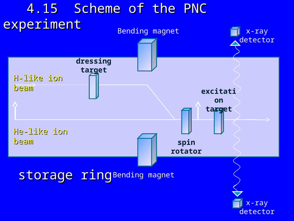
4.15 Scheme of the PNC experiment 4.15 Scheme of the PNC experiment

H-like ion beamH-like ion beam

He-like ion beamHe-like ion beam

Bending magnet

Bending magnet

dressingtarget

excitationtarget

x-raydetector

x-raydetector

storage ring storage ring

spin rotator

4.16 Observation time for the PNC effect4.16 Observation time for the PNC effect

Observation time to fix the PNC effect tobs (fix)

Number of events necessary to fix the PNC effect N(fix) = 108

Revolution time trev = 10-6 s

tobs (fix) · Nint / trev = N(fix)

tobs (fix) = N(fix) · trev / Nint = 108 · 10-6 /103 s = 0.1 s0.1 s

Observation timeObservation time to measure the PNC effect with to measure the PNC effect with accuracy 0.1%: accuracy 0.1%: ttobsobs (0.1%) (0.1%)

Number of eventsNumber of events necessary to measure the PNC effect with accuracy 0.1%: necessary to measure the PNC effect with accuracy 0.1%:

N(0.1%) = 10N(0.1%) = 1014 14

tobs (0.1%) = N(0.1%)·trev /Nint = 1014·10-6/103 s = 105 s ≈ 30 hours30 hours

5. ELECTRIS DIPOLE MOMENT (EDM) OF AN 5. ELECTRIS DIPOLE MOMENT (EDM) OF AN ELECTRON IN H-LIKE IONS ELECTRON IN H-LIKE IONS IN STORAGE RINGS5.1 EDM’S OF THE MUONS AND NUCLEI AT STORAGE

RINGS

I.B. Khriplovich Phys. Lett. B I.B. Khriplovich Phys. Lett. B 444444, 98 (1998), 98 (1998)

I.B. Khriplovich Hyperfine Interactions I.B. Khriplovich Hyperfine Interactions 127127, 365 (2000) , 365 (2000)

Y.K. Semertzidis Proc. of the Workshop on Frontier Tests of Y.K. Semertzidis Proc. of the Workshop on Frontier Tests of

Quantum Electrodynamics and Physics of theQuantum Electrodynamics and Physics of the

Vacuum, Sandansky, Bulgaria (1998)Vacuum, Sandansky, Bulgaria (1998)

F.J.M. Farley, K. Jungmann, J.P. Miller, W.M. Morse, Y.F. Orlov,F.J.M. Farley, K. Jungmann, J.P. Miller, W.M. Morse, Y.F. Orlov,

B.J. Roberts, Y.K. Semertzidis, A. Silenco and E.J. StephensonB.J. Roberts, Y.K. Semertzidis, A. Silenco and E.J. Stephenson

Phys. Rev. Lett. 93, 052001 (2004)

5.2 Spin precession of the particle in the 5.2 Spin precession of the particle in the external magnetic field external magnetic field HH : :Lab. frame: Lab. frame:

gg – gyromagnetic ratio (g=2 for leptons), qq – charge

Rest frame: Rest frame:

ωT - frequency of Thomas precession

(d(dss/dt)/dt)rest rest = = s ×s ×ΩΩμμ

Bargmann-Michel-Bargmann-Michel-

Telegdi (BMT) Telegdi (BMT)

equationequation

a = ½ g -1 For leptons a ≈ a = ½ g -1 For leptons a ≈ αα//ππ ≈ 10 ≈ 10-3-3

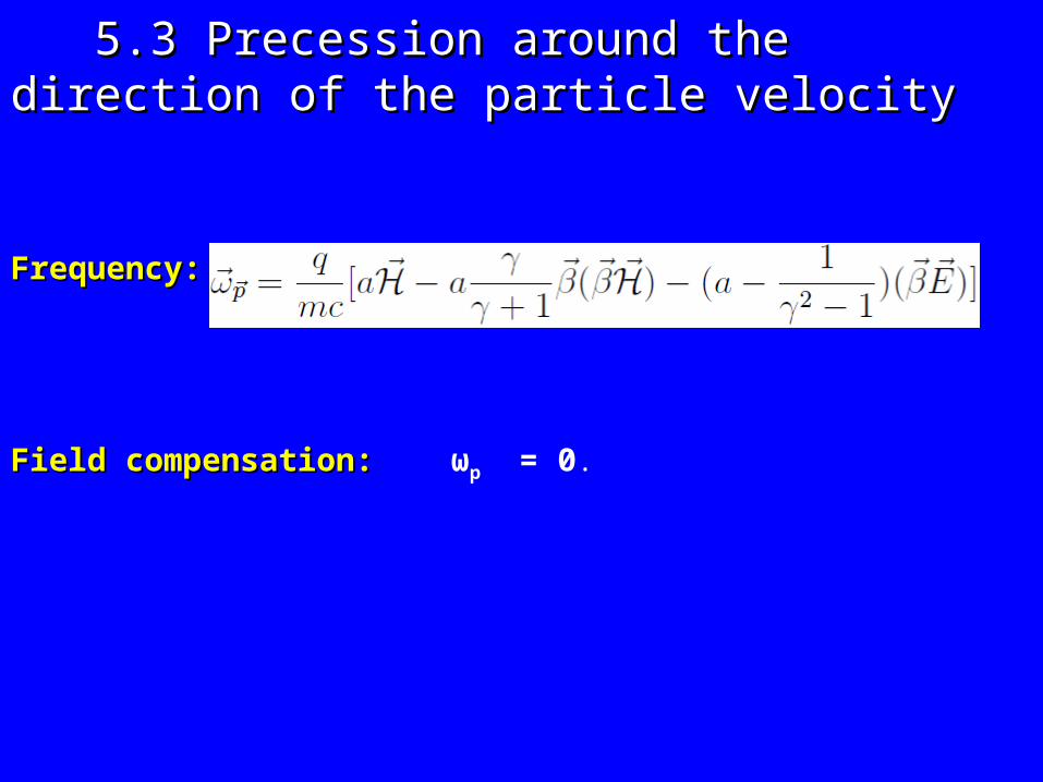
5.5.33 Precession around the direction of the Precession around the direction of the particle velocityparticle velocity

Frequency: Frequency:

Field compensation: Field compensation: ωp = 0.

5.4 Precession of the angular momentum of the 5.4 Precession of the angular momentum of the H-like HCI in storage ring H-like HCI in storage ring

H-like ion: particle with mass M (mass of the nucleus), charge q=Ze

and magnetic moment .

(magnetic moment of the electron)

Thomas precession can be neglected.

BMT equation:BMT equation:

Field compensation is not possible: for the vertical field 1 T the static radial

electric field 107 V/cm is necessary.

H-like ion with nuclear spin I : total angular momentum F

Kinematics will be defined by F

Dynamics will be defined by μ0

BMT equation:BMT equation:

Exact proof: Wigner-Echart theorem

5.5 EDM spin precession for H-like HCI5.5 EDM spin precession for H-like HCI

for any particle

For H-like HCIFor H-like HCI

Frequency of the EDM precession:

EDM:

If d dee ≈ 10 ≈ 10-28-28 e cm, ηη ≈≈ 10 10-17-17

5.6 EDM spin rotation angle 5.6 EDM spin rotation angle

IQA rotation in the plane IQA rotation in the plane xyxy due to the due to the

motional magnetic field motional magnetic field HHmm==ββ××EE

neglecting electron EDM. In theneglecting electron EDM. In the

absence of absence of EE the IQA is directed along the IQA is directed along

yy axis. axis. φφ – electron EDM rotation angle (in the plane – electron EDM rotation angle (in the plane yzyz) averages to zero due to ) averages to zero due to

the the HHmm rotation; compensating magnetic field rotation; compensating magnetic field HHcc is necessary. is necessary.

z

y

x

EHm

IQAy

x

EHm

IQA

z

φ-φ

IQA rotation in the plane IQA rotation in the plane xyxy due to the due to the

motional magnetic field motional magnetic field

+ IQA rotation in the plane + IQA rotation in the plane yzyz due to the due to the electron EDM. electron EDM.

Hc

5.7 Observation of the EDM effect in storage rings 5.7 Observation of the EDM effect in storage rings

A.A. ββ – active bare nuclei or HCI with – active bare nuclei or HCI with ββ – active nuclei and – active nuclei and

closed electron shells:closed electron shells:

Decay process: N* → N + e- + νz e

B. B. muon:muon:

Decay process: μ- → e- + νz e + νμ

Observation: asymmetry ζne

ζ – polarization of the nuclei (muon)

ne – direction of the decay electron emission

Both processes are P – violating. However they are due to the weak interaction.

Therefore no additional smallness

5.8 Observation of the electron EDM with H-like5.8 Observation of the electron EDM with H-like HCI in storage ring HCI in storage ring

Laser excitation of the HF excited level

1s1/2 F=2 → 1s1/2 F=3 for 15163Eu 62+

Decay is observed; decay time ~ 11 ms, then again excitation

sph – photon spin; νph - direction of the photon emission

(sph νph) = ± 1 chirality, or circular polarization

ζ – ion polarization vector; λ – degree of polarization

Qc = const; for 1s1/2 F=3 → 1s1/2 F=2 transition Qc = ½.

Asymmetry observed: Asymmetry observed: ζνζνphph ; ;

ifif circular polarization is fixed, there is no P-violation circular polarization is fixed, there is no P-violation..

Summation over circular polarizations (±) gives zeroSummation over circular polarizations (±) gives zero

Φ-Φ

-φ

φ

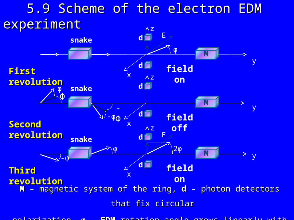
5.9 Scheme of the electron EDM experiment5.9 Scheme of the electron EDM experiment

MM – magnetic system of the ring, – magnetic system of the ring, dd – photon detectors that fix circular – photon detectors that fix circular

polarization, polarization, φφ – – EDM EDM rotation angle grows linearly with timerotation angle grows linearly with time

y

x

Edz

φsnake

d

M

First revolutionFirst revolution

x

dsnake

d

M

x

Ed

2φsnake

d

M

Second revolutionSecond revolution

Third revolutionThird revolution

field on

field off

field on-φ

φ

z

z

y

y

5.10 Estimates for the observation time5.10 Estimates for the observation time

Asymmetry Asymmetry A = A = λλ Q Qcc λ λ = F sin= F sinφφ ≈ F ≈ F φφ ( (φφ « 2 « 2ππ); F=3 for Eu); F=3 for Eu62+62+

φ φ = | = | ωωdd | t | tobsobs p p, p , p is the part of the ring where electric field is appliedis the part of the ring where electric field is applied

ωωd d is the frequency of the EDM caused spin precession is the frequency of the EDM caused spin precession

Numbers: E ≈ 10Numbers: E ≈ 1055 V/cm, p = l/L; l is the length of the field region; V/cm, p = l/L; l is the length of the field region;

L is the ring length; p = 0.001 (L = 100 m, l = 10 cm); HL is the ring length; p = 0.001 (L = 100 m, l = 10 cm); Hcc ≈ 300 gauss ≈ 300 gauss

These fields These fields EE, , HHcc applied within pL, do not disturb essentially the applied within pL, do not disturb essentially the

trajectory trajectory

| | ωωdd | ≈ | ≈ ηη 10 101010 s s-1-1

a)a) Let Let A ~ 10A ~ 10-5-5 ; ; ηη ~ ~ 1010-17-17 ,, dde e ~ 10~ 10-28-28 e cm e cm;; thenthen ttobsobs ~ 10 ~ 1055 ~ ~ 30 hours30 hours

b)b) Let Let A ~ 10A ~ 10-6-6 ; ; ηη ~ ~ 1010-19-19 ,, dde e ~ 10~ 10-30-30 e cm e cm;; thenthen ttobsobs ~ 10 ~ 1066 ~ ~ 1212 days days

6. CONCLUSIONS6. CONCLUSIONS

• PolarizationPolarization: for : for 1511516363EuEu62+ 62+ polarization timepolarization time

for the 100% polarization for the 100% polarization t tpolpol = 0.44 s = 0.44 s

Nuclear polarization, corresponding to Nuclear polarization, corresponding to

100% ion polarization: 100% ion polarization: 93%93%• PNC experimentPNC experiment

Time necessary for the observation of the PNC effect Time necessary for the observation of the PNC effect

ttobsobs PNCPNC ~ 0.1 s ~ 0.1 s

Time necessary for the measurement of the PNC effect Time necessary for the measurement of the PNC effect

with accuracy 0.1% with accuracy 0.1% (higher than in neutral Cs) (higher than in neutral Cs) ttobsobsPNCPNC ~ 30 hours ~ 30 hours

• Time necessary to observe Time necessary to observe electron EDMelectron EDM at the at the

level level 1010-28-28 e cm: t e cm: tobsobsEDM EDM ~~ 30 hours30 hours

Time necessary to observe Time necessary to observe electron EDMelectron EDM at the at the

level level 1010-30-30 e cm: t e cm: tobsobsEDM EDM ~~ 12 days12 days