SOUTHERN JOURNAL OF AGRICULTURAL ECONOMICS DECEMBER, 1985

A BIOECONOMIC SIMULATION APPROACH TO MULTI-SPECIES INSECT MANAGEMENT

William G. Boggess, Dino J. Cardelli, and C. S. Barfield

Abstract to develop and implement a methodologywith which to evaluate multi-species, non-Classical approaches to the economics of with which to evaluate multi-species, non-

pest management have focused almost ex- stochastic, managerial decision variables sub-ject to stochastic elements of weather andclusively on single-species models. This study the plant-sect sys elements of weather and

develops and implements a methodology with task the Florida Soybean Integated opwhich to evaluate multi-species, non-sto- tas, the Flora Soyean Integrated Cropchastic, managerial decisions subject to sto- Management (SICM) Model was used Wilk-chastic elements of the plant-insect system. eon t al. 1983b). Thismodel wasdesignedto integrate the effects of various soybeanMulti-species insect management strategies insect pests at the field level under varying(combinations of scouting interval, threshold w , c a s value, and choice of pesticide) are analyzed using a physiological mechanistic soybeanplant growth model coupled to three insectpopulation dynamics models. Preliminary re- PREVIOUS PEST MANAGEMENTsuits indicate that net returns are maximized MODELING RESEARCHand variance is reduced with lower thresh- Biological simulation models of insects andolds and more frequent scouting than current crops are relatively recent developments.recommendations. Early modeling efforts begun in the mid-Key words: pest management, multi-species, 1970's focused on controlling boll weevils

simulation, stochastic domi- in cotton. Brown et al. provide an excellentnance. overview of the development of the Missis-

,Classical~ apoce sippi cotton growth and insect dynamicClassical approaches to economics have models. Gutierrez et al. were the first to

not focused adequately on development of publish an analysis of cotton pest manage-tools (e.g., models) for agricultural deci- ment based on a detailed biological simu-sionmaking under multiple insect species lation model. Talpaz et al. followed closelyconditions. Far more emphasis has been behind with an economic optimization modelplaced on development of management strat- which incorporated a detailed plant-pest in-*egies for single insect species (Watt; Carlson; teractive system with a pesticide controlHall and Norgaard; Hueth and Regev; Mar- scheme. The model used a temperature de-solan and Rudd; Talpaz et al.). However, in pendent boll weevil model combined withmany production systems, multiple insect a mechanistic fruit drying and cotton fruitingpests are prevalent. In these cases, manage- model.ment may be much more complex than single Marsolan and Rudd developed one of thespecies management since: (1) the pests may earliest soybean insect dynamics models. Theyoccur together or at different times in the used a distributed-parameter population dy-season, (2) the pests may attack the plant in namics model of the southern green stinkbugdifferent ways (e.g., defoliators vs. pod feed- [Nezara viridula (L)] to evaluate optimalers), and (3) the pests may exhibit different control strategies. The model described thelevels of susceptability to controls. mortality, fecundity, and movement as an age

This study represents a first step in multi- dependent function and assumed instanta-species insect management. The objective is neous control by methyl-parathion.

William G. Boggess is an Associate Professor of Food and Resource Economics, University of Florida; Dino J.Cardelli is a Corporate Economist, Tropicana Inc., Bradenton, Florida; and C. S. Barfield is an Associate Professorof Entomology, University of Florida.

Florida Agricultural Experiment Station Journal Series No. 6439. This work was supported by the Institute ofFood and Agricultural Sciences, University of Florida and by EPA Grant No. CR-806277-02-0.

43

Reichelderfer and Bender were the first to the risk associated with alternative control

use biological simulation in the evaluation strategies can be a critical factor in the eval-

of pest control in soybeans. Predator-pest uation and choice of strategies. The simu-

relationships of the Mexican bean beetle were lation model facilitates evaluation of

incorporated into a microanalytic model to alternative strategies under stochastic con-

generate output response surfaces of alter- ditions, allowing empirical derivation of

native biological and chemical control strat- probability distribution functions for each of

egies. The response surfaces were combined the strategies. The various probability distri-

with cost data to construct benefit-cost ratios bution functions can then be compared using

for intraseasonal control options. stochastic dominance procedures in order to

In the 1980s, several articles advanced the determine risk efficient strategies. No distri-

development of dynamic management-ori- butional assumptions are required in order

ented models. Zavaleta and Reusink exam- to apply stochastic dominance rules.

ined potential gains derived from biological Two stochastic dominance rules, first de-

means of control, as well as the introduction gree and second degree are applied in this

of host plant resistance in their model. Shoe- study. First Degree Stochastic Dominance

maker developed a stochastic dynamic pro- (FSD) states, Any alternative B is preferred

gramming model to analyze the integrated to any alternative A if FB(x) • FA(x) for

control of alfalfa weevils in central New York. all values of x, i.e., if the cumulative prob-

The management alternatives considered in- ability of B lies to the right of A. The only

cluded biological control by the parasitoid assumption required to use FSD is that the

Bathyplectes curculionis, cultural control by decisionmaker prefers more to less (Anderson

harvesting, and chemical control by insec- et al.). Second Degree Stochastic Dominance

ticides. Wilkerson et al. (1983a) developed (SSD) states, Alternative B is preferred to

a time-dependent dynamic model for eval- Alternative A for all risk averters if the

uating within-season management decisions cumulative difference between FA(x) and

for velvetbean caterpillars in soybeans. FB(x) is non-negative over the domain ofX. Mathematically, SSD requires that:

xMODEL AND PROCEDURES (1) J [FA(x)-FB(x)] dx > 0

The present study uses a multi-speciesbioeconomic simulation model (Wilkerson for all values of x. The SSD rule assumes that

et al., 1983b) to build on the previous single- the decisionmaker prefers more to less and

species models presented in the literature. is risk averse (Anderson et al.).

This modeling approach avoids two of the Strategies were constructed to illustrate

major limitations of the neoclassical theory how the model may be used to evaluate the

of the firm as it relates to the problem of sensitivity of profit to various combinations

evaluating multiple-species management of population threshold levels, scouting fre-

strategies. First, the plant-insect ecosystem is quencies, and pesticide types and rates. Forty

a complex, dynamic system in which timing strategies were developed to account for five

is a critical element. The SICM simulation threshold levels of total worms (0, 5, 10,

model is essentially a computer model of the 15, and 20 per 3 row feet), four scouting

elementary processes that define the soybean frequencies (3, 5, 7, and 10 days) and two

production system. In this approach, the sim- chemical combinations. These combinations

ulation model replaces the classical produc- were designed to bracket the current rec-

tion function and is used to empirically derive ommendation of 12 worms and a 7-day scout-

the relationships between the various insect ing interval (Johnson et al.). "Total worms"

management strategies, yields, and pesticide is defined as the sum of medium and large

applications. These empirical relationships velvetbean caterpillar larvae plus large corn

are used to determine the profit maximizing earworm larvae. The southern green stinkbug

strategies, the demand for pest control, and treatment threshold was set at 1 adult per 3

the marginal cost of pest control under var- row feet which is the current extension rec-

ious influx and price conditions. ommendation (Johnson et al.).

The second limitation of the classical ap- For each strategy, both an early season and

proach is that it ignores risk. Given the sto- a late season pesticide type were chosen. The

chastic nature of weather and insect influxes, early (pre-bloom) pesticide is used to control

44

foliage feeders while the late (post-bloom) weather, soil, pest and crop conditions, andpesticide is primarily used to control pod are linked mathematically by a series of dif-feeding insects. Two pesticide combinations ferential equations that depend on the phen-were chosen to examine the effects of pes- ological phase of crop development. Becauseticide types. Methomyl was the early pesti- of the length and complexity of the statecide used in both pesticide combinations, equations describing this system, readers in-Methyl-parathion and acephate are both rec- terested in a more detailed explanation areommended by the Extension Service for late referred to Wilkerson et al. (1983c).season stinkbug and corn earworm control The usefulness of the SICM model is ob-(Johnson et al.). Acephate is more expensive viously dependent upon the accuracy of thethan methyl-parathion but has a longer re- crop growth simulation model results. Vali-sidual effect on both the pest and predator dation of the crop growth model was per-populations. formed by comparing simulated yields with

The primary stochastic variables affecting observed experimental yields over a 3-yearthe plant-insect ecosystem are related to period. A correlation between the simulatedweather. The strategies were evaluated over and observed yields of 0.98 was obtained.10 years (1954-1963) of actual daily radia-tion, precipitation, and maximum and min-imum temperatures. Insect Mode

The influx timing and intensity of insect Three insect' models are linked to the croppests are also important stochastic variables, growth model. These models simulate insectHowever, there are insufficient data to sta- population dynamics (fecundity, develop-tistically estimate probability distributions. ment, and mortality) and link the insects toIn order to provide sensitivity analyses, in- the crop via consumption of leaves and pods.dependent, uniform distributions were as-sumed for both influx intensity and initialinflux timing. Three levels of velvetbean cat- Insect Developmenterpillar influx intensity (small, average, and Velvetbean caterpillar populations (VBC)heavy) were specified. The specific values are divided into six developmental stages:were determined from light trap data under eggs, small larvae (instars 1-2), medium lar-actual conditions (Wilkerson et al., 1983b). vae (instars 3-4), large larvae (instars 5-6),In addition, three levels of initial influx tim- pupae, and adults. Within each growth stage,ing of velvetbean caterpillar (early, on-time, an age structure is maintained. Insects moveand late) were specified. Julian dates of the from age block to age block within a giveninfluxes are 179 (June 29), 202 (July 22) growth stage until they have accumulated aand 219 (August 10) (Wilkerson et al., sufficient number of physiological days to1983b). advance to the next developmental state

Current components of the SICM model (Wilkerson et al., 1985).include crop growth, insect, tactics (pesti- The corn earworm (CEW) populationcides and irrigation), and economics. An model developed by Stinner et al. uses aoverview of each of these components fol- variation in development time for a givenlows with the reader being referred to the temperature to simulate the change of gen-appropriate literature for specific details. erations and prevent discrete overlapping.

The model accumulates proportions of in-sects that entered a given stage on previous

Soybean Crop Growth Model dates developing to the next stage on a spe-(SOYGRO) cific later date. In the simulation, insect dens-

ities are calculated daily, starting with theSOYGRO is a process oriented growth and first date of influx.

yield model which comprises the core of the Rudd modeled the emergence of stinkbugSICM model. Physiological processes of pho- individuals from a stage by an emergencetosynthesis, respiration, tissue synthesis, ni- function, which is the fraction or percentagetrogen remobilization, and senescence are of those individuals that have progressed tomodeled. These processes are coupled to the next stage by time t. The derivative of

'Insect components include velvetbean caterpillars, Anticarsia genmatalis [Hubner]; corn earworm, Heliothis zea[Boddie]; and southern green stinkbug, Nezara viridula [L].

45

this function with respect to time is an age- where 1 is the number of pesticide appli-dependent probability distribution that de- cations which have been made to date, andscribes the progression of the individuals siTk (t - tk) is the proportion of the popu-through stages; i.e., the probability of an lation, stage i, present t - tk days after spray-individual emerging from a stage at time t. ing, which survive the effect of pesticide TkThe probability distribution for the southern (applied at time tk). The siTk (t - tk) repre-green stinkbug was obtained from develop- sents input data for each pesticide type andment data by Kiritani et al. and Herzog et al. insect stage.

Predator populations are affected in a sim-ilar manner. First the model computes the

Mortality factor SpTk by which predator populations arereduced below those of an untreated field

At present, mortalities inflicted by preda- (t-t) days after pesticide T, was applied.tors, pesticide applications (also Bacillus Thus, the number of predators present in thethuringiensis Berliner), and food shortage field at time t is calculated as:are incorporated into the model. Function-ally, mortality is represented as: (t t),

(4) PR = PR..x(t) ° SpTk (t - tk),(2) i = (1-SiB)(1-SiF)(1 -Sip)(1 -ST), k=

where it is the proportion of insects in de- where PRm,(t) is the number of predatorsvelopment stage i which die, and the si's which will be present in the field at time t,represent the proportion of the population if the field was not sprayed.in stage i which survive the particular mor-tality factors (background (B), food (F), pre-dators (P), and pesticides (T), respectively). Economics Model

The economics model integrates the effectsConsumption of a particular management strategy on crop

yield and input use with prices to determineThe insect models are tied to the crop net returns. This value is calculated by sub-

model through leaf and pod consumption. tracting the total variable costs incurred dur-Consumption of pods directly reduces crop ing the season from the gross return. Theyield; whereas, leaf consumption (defolia- costs are broken down in the model into: (1)tion) reduces yields via reduced photosyn- variable production costs other than insectthesis. Consumption rates are 0.06, 3.0, and control, (2) scouting costs, and (3) variable48.0 cm2/day for small, medium, and large pest management costs.larvae, respectively. These values were ob- Variable production costs per acre exclud-tained by converting fresh leaf weight con- ing insect control costs are calculated as:sumption from Moscardi to dry weight, andthen to area using relationships developed (5) Cm = 111.50 + [2.98 Pgby Boote. + 9.20 Pd] 1.15,

where Cm = variable production costs ($/acre) excluding insect control costs,

Tactics Model Pg = price of gasoline per gallon andPd = price of diesel fuel per gallon. Equa-Various tactics can be used to control pest = price of diesel fuel per gallon. Equa-

populations and reduce crop stress. In par- tion (5) is derived from a North Florida soy-ticular, pesticides can be used to manage bean cost of production budget prepared byinsect populations and irrigation can be used Hewitt.to control water stress. Pesticides affect pest Scouting costs are based on the commercialinsect mortality directly (Pi T) and also indi- rate of $5 per acre per year for a once-a-rectly by decreasing predator populations. week scouting program. The number of tripsMortality of target insects due to pesticide was divided into the $5 per acre per yearspraying is calculated as: costs to yield a marginal cost of $0.45 per

trip per acre. Total scouting costs are given1 by:

(3) PIT,(t) = 1.0 - sT (t - tk),k= k (6) Cs = $0.45 * number trips made.

46

Variable costs of pest control (pesticide 20 worms, net returns steadily decrease fromand application costs) are calculated as: $83.92 to $58.45 and the standard deviation

7- Cm =P * N) + (P * N, oof net returns increase from $88.95 to $94.96,(7) Cpm = (Pm + N) + (Pap + N), Table 1. In a similar fashion, as the scouting

where Cpm = total seasonal variable costs interval is increased (holding threshold con-of pest control ($/acre), Pm = cost ofchem- stant at 10 worms and using methyl-para-icals applied per acre per spray application, thion), mean net return decreases and thePap = application cost per acre, and standard deviation of net returns increases.N = number of spray applications per acre. As the scouting interval increases from 3 to

5 to 7 to 10 days, mean net return decreasesfrom $78.35 to $72.44 to $71.88 to $69.11,

RESULTS respectively, and the standard deviation ofper acre net returns increases from $92.06

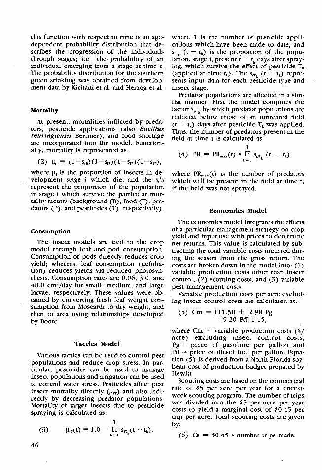
Initially, each of the forty strategies was to $95.02 (strategies 7, 9, 11, and 29, Tablesimulated over all nine insect influx condi- 1). Similar relationships exist between thetions and all 10 weather years. A strategy mean and standard deviation of yields andconsisting of a 3-day scouting interval, 5 scouting interval and between the mean andworms per 3 row feet threshold, and a meth- standard deviation of yields and thresholdomyl, methyl-parathion pesticide combina- level.tion maximizes expected net returns for allstrategies evaluated, Table 1. There is con- Risk Considerationssiderable variation in mean net returns overthe 40 strategies, ranging from a low of The relative magnitude of the standard de-$-15.82 per acre to a maximum of $83.92 vatons of net returns indicates that the sto-viations of net returns indicates that the sto-

per acre. chastic nature of weather, pest levels, andThe top eight strategies had expected net timing greatly influence net returns (i.e., the

returns within 10 percent of the optimal coefficients of variability are greater than 1.0strategy and the top 18 strategies hd ex- for the majority of the strategies). This sug-pected net returns within 20 percent of the t tt risk considetions may play anoptimal strategy Table 1. Ofthe top 10 strat- important role in selecting strategies. For

timl seigy, Tabe threshol ve toexample, it may be desirable to switch strat-egies, eight had a threshold of five worms. e egies once the timing and magnitude to theNote that the yield obtained with treatment once the timing and magnitudeo toe eat a five-worm threshold (Strategy 1) is greater this p ossibility cumulative probailit func

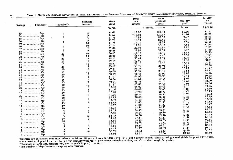
this possibility, cumulative probability func-than the yields obtained with calendar treat- tions of the various strategies were derivedments (strategies 33-40). This is an example from various velvetbean caterpillar influxof the so called "pesticide treadmill." Early conditions. Inapproximately half of the in-and heavy pesticide treatments deplete the flux conditions, the overall "optimum" strat-predator complex. This allows more rapid egy (5 worms, 3 days, methyl-parathion)resurgence of the pest insects as well as dominated the other strategies by second de-secondary breakouts of normally minor pests. gree stochastic dominance. An example isSince the pesticides do not kill all of the the case of a small, late influx, Figure 1.target insects, there continues to be damage. However, under other influx conditions, al-The net effect of the more rapid resurgence ternative strategies outperformed the 5-worm,and secondary outbreaks is a reduction in 3 days, methyl-parathion strategy. In the caseyield. The reduction in yield is greater the of a heavy, on-time influx, the 5-worm, 7longer the scouting interval (interval be- days, methyl-parathion strategy dominated bytween calendar sprays). first degree stochastic dominance, Figure 2.

Results demonstrate a systematic relation- The latter case illustrates the potential valueship between net returns and scouting in- of information about uncertain events (e.g.terval and between net returns and threshold insect influxes). If you know the influx islevel. As the threshold level is increased from heavy and on-time, a 7 day scouting interval5 worms (holding scouting interval and pes- matches up very well with the influx andticide type constant), mean net return de- development of VBC. The crop is scouted atdines and the standard deviation of net returns just the right time to catch the pest at dam-increases. These results can be seen by com- aging levels. This allows very effective con-paring strategies 1, 7, 13, and 21. As the trol with an average of one less pesticidethreshold is increased from 5 to 10 to 15 to application than would be applied under a

47

rP^ ~TABLE 1. MEANS AND STANDARD DEVIATIONS OF YIELD, NET RETURNS, AND PESTICIDE COSTS FOR 40 SIMULATED INSECT MANAGEMENT STRATEGIES, SOYBEANS, FLORIDAa

Mean Mean St. dev.

Scouting Mean net pesticide Std. dev. net

Strategy Pesticideb Thresholdc interval yield returns costs yield returnsbu./ac. - per ac.-

33 .................... Mp 0 3 34.62 -15.82 129.49 11.86 82.2734 ..................... Or 0 3 34.62 -- 15.82 129.49 11.86 82.27

35 ................. Mp 0 5 31.73 10.93 82.50 9.97 69.50

36 ..................... Or 0 5 31.73 10.93 82.50 9.97 69.5039 ................... Mp 0 10 27.74 12.21 53.33 7.54 52.36

40 ..................... Or 0 10 21 53.33 7.4 52.3637 .............. p...... M 0 7 29.88 22.91 57.59 8.87 61.89

38 ..................... Or 0 7 29.88 22.91 5759 8.87 61.8927 .................... Mp 2 0 10 26.65 9527 ...... ·. ········--·- Mp 20 10 26.65 41.12 16.79 13.92 95.53

28 ..................... Or 20 10 28.00 45.88 21.46 12.60 87.94

25 .................... Mp 20 7 28.12 50.44 17.74 13.79 95.17

26 ..................... Or 20 7 29.19 52.99 2270 12.66 88.8131 .................... Mp 15 10 2857 53.16 18.6 13.72 94.4131 .... ··········-·-··- Mp 15 10 28.57 53.16 18.16 13.72 94.41

24 ..................... Or 20 5 29.62 53.72 2495 12.37 87.26

23....................Mp 20 5 29.11 54.21 20.91 13.67 94.27

32 ..................... Or 15 10 29.68 55.94 2315 12.84 88.82

21 .................... Mp 20 3 30.29 58.45 24.94 13.83 94.96

16 ..................... Or 15 5 31.07 61.93 26.90 1274 89.23

17 ..................... Mp 15 7 30.24 63.61 19.43 13.6 93.94

18 ..................... Or 15 7 30.94 6373 24.17 12.69 88.89

30 ..................... Or 10 10 31.32 6500 25.54 12.93 89.6622 ..................... Or 20 3 32.02 65.07 30.43 13.16 89.96

15 .................... Mp 15 5 31.06 66.08 22.66 13.88 95.6010 ..................... Or 10 5 32.20 67.98 28.76 12.42 87.1529 .................... Mp 10 10 31.25 69.11 20.97 13.73 95.02

12 ..................... Or 10 7 32.15 70.08 26.30 1236 86.83

13 .................... Mp 125 3 3.8013 .···.·-- ············ Mp 15 3 32.39 71.10 26.93 13.60 93.80

14 ..................... Or 15 3 33.15 71.45 31.95 13.19 89.88

11 .................... Mp 10 7 31.72 71.8814.00 96.47

9 .................... Mp 10 5 32.23 72.44 24.53 13.56 93.62

4 ..................... Or 5 5 33.65 74.49 32.37 12.17 85.02

6 ..................... Or 5 7 33.48 76.14 29.56 12.25 85.85

20 ..................... Or 5 10 33.63 76.78 29.96 12.80 87.15

8 ..................... Or 10 3 34.20 77.44 33.31 12.59 86.38

7 .................... Mp 10 3 33.66 78.35 28.63 13.35 92.06

5 .................... Mp 5 7 33.20 79.39 24.33 13.71 94.57

2 ..................... Or 5 3 35.09 80.34 36.61 12.05 83.473 .................... MP 5 5 34.15 81.77 28.62 13.23 91.10

19 .................... Mp 5 10 33.70 82.62 24.63 13.20 90.101 .................... Mp 5 3 35.04 83.92 32.66 12.92 88.95

aStatistics are calculated over nine influx conditions, 10 years of weather data (1954-63), and a growth model validated using actual yields for years 1970-1980.bCombination of pesticides used for a given strategy with MP = (Methomyl Methyl-parathion) and Or = (Methomyl, Acephate).cThreshold of large and medium VBC and large CEW per 3 row feet.-'The number of days between sampling observations.

*1 "":A8~0 1(5 worms, 7 days, Methyl-parathion) -- '

0.75-

0- .

0.25f '--- (5 worms, 3 days, Methyl-parathion)

0.00 -——_______ I

-4.80 0.00 40.00 80.00 120.00 160.80 200.00 248.00Net Returns/Acre

Figure 1. Cumulative Probability Functions of Net Returns for a Small Late Influx of VelvetbeanCaterpillars in Soybeans, Florida.

three day scouting interval with an additional effect of scouting, treatment threshold, andsavings of $6.30 in scouting costs. control tactic applied on pest populations.

Various combinations of these parameters willresult in varying degrees of pest controls (e.g.

Pest Control Demand and Marginal different levels of pest populations over time).Cost Curves If any two of these three strategy variables

are held constant, conditional marginal valueDue to the dynamic nature of the soybean product and marginal cost curves can be

production process, there is no single derived derived.demand or marginal cost curve for pest con- For example, the maximum net return istrol. Rather, pest control is the cumulative generated from scouting on a 3 day interval,

49

1 .00 (5 worms, 3 days, Methyl-parathion) -—

J3 |«^^^^ > +-— (5 worms, 7 days, Methyl-parathion)

0.25

g //8

-4.00 0.00 40.80 80.00 120.00 t160.00 20.00 248.00Net Returns/Acre

Figure 2. Cumulative Probability Functions of Net Returns for a Heavy, On-Time Influx of Velvetbean

Caterpillars in Soybeans, Florida.

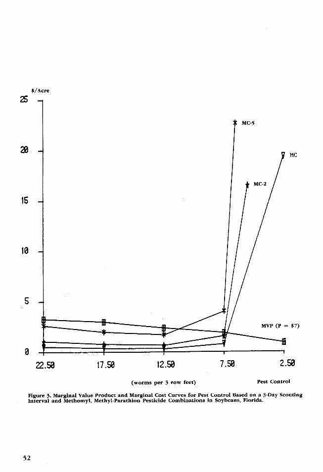
and treating at 5 worms per 3 row feet with The base marginal cost curve (MC) andmethomyl and methyl-parathion. By holding base marginal value product curve (MVP) arethe scouting interval and pesticide type con- illustrated in Figure 3. The maximum netstant, the conditional demand and marginal return threshold is approximately 7 wormscost curves for treatment threshold are de- per 3 row feet. This indicates that the max-rived as a function of insect population. The imum net return occurs between the 5 wormscurves are derived empirically from the sim- per 3 row feet and the 10 worms per 3 rowulation data using discrete interval calcula- feet points that were actually simulated. Usetions of the marginal product and marginal of the MVP and MC curves allows examina-cost relationships, Table 2. tion of the surface in a single dimension

50

TABLE 2. INTERVAL CALCULATIONS OF THE MARGINAL COST AND MARGINAL VALUE PRODUCT OF PEST CONTROL, MULTI-SPECIES INSECT MANAGEMENT MODEL FOR SOYBEANS, FLORIDA

Interval values Mean Internal valuesMean pesticide

Thresholda yield MP MVP-3b MVP-7b MVP-12b costs MCC MC-2c MC-5cbu./ac. bu./ac. ------------------------------------------------------------------------------------ ac---------------

No control(50.0) ............... 13.49 0

.56 1.68 3.92 40.32 .83 1.66 4.1520.0 .............. 30.29 24.94

.43 1.29 3.01 5.16 .40 .80 2.0015.0 ............... 32.38 26.93

.34 1.02 2.38 4.08 .34 .68 1.7010.0 ............... 33.66 28.63

.27 .81 1.89 3.24 .80 1.60 4.005.0 ............... 35.04 32.66

.13 .39 .91 1.56 19.37 38.74 96.850.0 ............... 35.69 131.25

'Number of large and medium VBC and large CEW per 3 row feet.bMarginal value product with soybean prices at $3, $7, and $12 per bushel, respectively.cMarginal cost of pest control averaged over 90 observations (MC), two times the average marginal cost (MC-2), and five times the average marginal cost (MC-5).

,l

$/Acre

25

MC-5

MC

MC-2

15

MVP (P = $7)

22.50 17.50 12.50 7.50 2.50

(worms per 3 row feet) Pest Control

Figure 3. Marginal Value Product and Marginal Cost Curves for Pest Control Based on a 3-Day ScoutingInterval and Methomyl, Methyl-Parathion Pesticide Combinations in Soybeans, Florida.

52

between the simulated reference points with- mum net return strategy of 7 worms and aout the additional expense. If additional re- 3-day scouting interval calls for more fre-finement of the surface is desired, interim quent scouting and treatment at a signifi-points (e.'g. 7 worms per 3 row feet) can be cantly lower threshold than the currentsimulated. Extension Service recommendations (John-

Several factors can affect either the MVP son et al.) of weekly scouting and a treatmentor MC curves causing them to shift upward threshold of 12 worms. The lower thresholdor downward. Factors which affect the mar- results in a 19 percent increase in expectedginal value product curve include: (1) net returns and a 7 percent decrease in thechanges in the basic processes which deter- standard deviation of net returns. However,mine yield (e.g., insect population dynamics, the lower threshold and more frequent scout-scouting interval, or pesticide type) and (2) ing result in approximately a 60 percenta change in the price of the output. The increase in pest control costs. This thresholdmajor act the p of is for factors affecting the position lepidoptera (or larval)marginal cost curve are the price of inputs insects and is defined in conjunction with ainto the pest control process (e.g., chemicals, threshold of 1 adult per 3 row feet for thescouting, and application). An increase (de- p d stem feed southern green stink-crease) in any one of these prices will shift bug. Second, no one strategy is optimal for

bug. Second, no one strategy is optimal forthe MC curve up (down. all VBC influx conditions. This suggests re-

Table 2 presents marginal value productsTable presentsmargalvalueproducts search that enables better prediction for VBCcalculated on the basis of soybean prices of i i ii$3, $7, and $12 per bushel. Note that all gudes and timings could yield

$3, $7, and $12 per bushel. Note that all -sizable returns. Third, as the scouting intervalthree marginal value product curves intersect thre marginal svaue prouct curve inters be- decreased, holding threshold constant, thethe marginal cost curve in the interval be-andard de-tween 10 and 5 worms, indicating that the a net returns creased standard de-maximum net return threshold is quite robust viations of net returns decreased indicatingto changes in output price. that given current prices, the value of ad-

Table 2 also presents marginal cost values ditional information (scouting) exceeds thecalculated on the basis of two- and five-fold cost and that additional information reducesincreases in the prices of all pest control risk Finally, the economic optimal thresholdinputs. These curves are represented as MC- is quite robust with respect to input and2 and MC-5 in Figure 3. As input prices output price changes. The threshold variedincrease, the optimal threshold increases. less than one worm as soybean prices variedHowever, the optimal strategy is quite robust from $3 to $12 or as pest control costs dou-to a twofold increase in pest control costs. bled.The threshold value increases only slightly Research is on-going to refine and validatecompared to the original marginal cost curve. the insect model parameters and to furtherA fivefold increase in all pest control input field test the results. Perhaps the most sig-prices is required before the optimal thresh- nificant aspect of this study is that it dem-old increases significantly from approxi- onstrates the ability of bioeconomicmately 7 worms to approximately 11 worms simulation models to integrate multiple cropper 3 row feet. stresses and to provide a vehicle for evalu-

ating multi-species insect management strat-egies. Initial analyses such as those presented

CONCLUSIONS in this study are particularly useful in dem-

Bioeconomic, process-level simulation onstrating the validity of the approach, gen-models are effective tools for integrating mul- erating research hypotheses for field testing,tiple crop stresses and for evaluating man- and for evaluating the sensitivity of the modelagement strategies. The approach explicitly to various parameters. This provides a frame-recognizes the critical time dependencies of work for more effective use of the limitedthe biological system and facilitates evalua- resources available for biological field re-tion of the profitability and risks of alternative search. Subsequent refinements in and vali-management strategies. dation of the model will provide additional

The results of this particular application confidence in the specific results.yield several preliminary conclusions and re- The results presented in the study are spe-searchable hypotheses. Foremost, the maxi- cific to North Florida conditions. The basic

53

model structure, however, is appropriate for been released to Illinois, Mississippi, Geor-other regions. Versions of the model have gia, Arkansas, Colorado, and Kentucky.

REFERENCES

Anderson, Jock R., John L. Dillion, and Brian Hardaker. Agricultural Decision Analysis,Iowa State University Press, Ames, Iowa, 1977.

Boote, K. J. Unpublished data, Agronomy Department, University of Florida.Brown, L. G., R. W. McClendon, and J. W. Jones. "Cotton and Insect Management Simulation

Model." Chapter 17 in Cotton Insect Management with Special References to theBoll Weevil, Edited by R. L. Ridgway, R. P. Lloyd and W. H. Corss, USDA, ARS, AgriculturalHandbook 589, pp. 437-80, 1983.

Carlson, G. A. "A Decision Theoretic Approach to Crop Disease Prediction and Control."Amer. J. Agr. Econ., 52(1970):216-23.

Gutierrez, A. P., T. F. Leigh, Y. Wang, and R. D. Cave. "An Analysis of Cotton Productionin California: Lygus Hesperus Injury-An Evaluation." Can. Entomol., 109(1977):1,375-86.

Hall, D. C. and R. B. Norgaard. "On the Timing and Application of Pesticides." Amer. J.Agr. Econ., 55(1973):198-201.

Herzog, D. C., L. D. Newsom, and R. M. McPherson. Unpublished data, 1975.Hewitt, Tim. "Budgets Generated for the Farm System Lab." Dept. of Food and Resource

Econ., University of Florida, 1983.Hueth, D. and U. Regev. "Optimal Agricultural Pest Management with Increasing Pest

Resistance." Amer. J. Agr. Econ., 56(1974):543-50.Johnson, F. A., D. C. Herzog, and R. K. Sprenkel. "Soybean Insect Control." Extension

Entomology Report #58, University of Florida, Gainesville, May, 1984.Kiritani, K. N., N. Hokyo, and K. Kiroma. "Survival Rate and Reproductivity of Adult Southern

Green Stinkbug, Nezara viridula, in the Cage." Jap. J. Appl. Entomol., 7(1963):113-8.

Marsolan, N. F. and W. G. Rudd. "Modeling and Optimal Control of Insect Pest Populations."Math Biosciences, 30(1976):231-44.

Moscardi, F. Effect of Soybean Crop Phenology on Development, Leaf Consumption, andOviposition ofAnticarsia gemmatalis Hubner, Ph.D. dissertation, University of Florida,Gainesville, 1979.

Reichelderfer, K. H. and F. E. Bender. "Application of a Simulation Approach to EvaluatingMethods for the Control of Agricultural Pests." Amer. J. Agr. Econ., 61(1979):258-67.

Rudd, W. G. "Status of Systems Approach to Pest Management." Ann. Rev. Entomol.,21(1976):27-44.

Shoemaker, C. A. "Optimization Analysis of the Integration of Biological, Cultural, andChemical Control of Alfalfa Weevil ( Coleoptera curculionidae )." Env. Entomol.,21(1983):286-95.

Stinner, R. E., R. L. Rabb, and J. R. Bradley. "Population Dynamics of Heliothis zea (Boddie)and H. virescens (F.) in North Carolina: A Simulation Model." Env. Entomol.; 3,1(1974):163-8.

Talpaz, H., G. L. Curry, P. J. Sharpe, D. W. DeMichele, and R. E. Frisbie."Optimal PesticideApplication for Controlling the Boll Weevil on Cotton." Amer. J. Agr. Econ.,60(1978):469-75.

Watt, K. E. F. "The Use of Mathematics and Computers to Determine Optimal Strategy andTactics for a Given Insect Pest Control Problem." Can. Entomol., 96(1964):202-20.

Wilkerson, G. G., J. W. Mishoe, J. W. Jones, W. G. Boggess, and D. P. Swaney. "Within-Season Decisionmaking for Pest Control in Soybeans."Agr. Eng. Dep. Paper No. 83-4044, University of Florida, 1983a.

Wilkerson, G. G., J. W. Mishoe, J. W. Jones, J. L. Stimac, D. P. Swaney, and W. G. Boggess."SICM Florida Soybean Integrated Crop Management Model: Model Description User'sGuide." Agr. Eng. Dep. Rpt. AGE 83-1, University of Florida, November, 1983b.

54

Wilkerson, G. G., J. W. Jones, K. J. Boote, K. T. Ingram, and J. W. Mishoe."Modeling SoybeanGrowth for Crop Management." Transac. ASAE; 26, 2(1983c):562-8.

Wilkerson, G. G., J. W. Mishoe, andJ. L. Stimac. "Modeling Velvetbean Caterpillar Populationsfor Crop Management." 1985 (In Review).

Zavaleta, Luis R. and William G. Ruesink. "Expected Benefits from Non-chemical Methodsof Alfalfa Weevil Control." Amer. J. Agr. Econ., 62(1980):801-5.

55

56