A better method to enforcemonotonic constraints in

regression and classification trees

Auguste, Charles1, Smirnov, Ivan2, and Malory, Sean2

1IMI - Departement Ingenierie Mathematique et Informatique,Ecole des Ponts ParisTech2Independent Researcher

November 1, 2020

Abstract

In this report we present two new ways of enforcing monotone con-straints in regression and classification trees. One yields better resultsthan the current LightGBM, and has a similar computation time. Theother one yields even better results, but is much slower than the cur-rent LightGBM. We also propose a heuristic that takes into account thatgreedily splitting a tree by choosing a monotone split with respect to itsimmediate gain is far from optimal. Then, we compare the results withthe current implementation of the constraints in the LightGBM library,using the well known Adult public dataset. Throughout the report, wemostly focus on the implementation of our methods that we made forthe LightGBM library, even though they are general and could be imple-mented in any regression or classification tree.

The best method we propose (a smarter way to split the tree coupledto a penalization of monotone splits) consistently beats the current imple-mentation of LightGBM. With small or average trees, the loss reductioncan be as high as 1% in the early stages of training and decreases toaround 0.1% at the loss peak for the Adult dataset. The results would beeven better with larger trees. In our experiments, we didn’t do a lot oftuning of the regularization parameters, and we wouldn’t be surprised tosee that increasing the performance of our methods on test sets.

1

1 Results

1.1 Summary of the important results

Figure 1: Loss and AUC vs. number of iterationsrelative to the constrained LightGBM baseline, forour best method and the unconstrained method, on

the train and test sets

On figure 1 are represented the most important results of the report. Overall,our best method generates a consistent and significant loss reduction, whichalso helps us improve common metrics. Therefore we think our method shouldbecome the standard for enforcing monotone constraints, and replace the currentLightGBM method.

2

1.2 Dataset and preprocessing

The Adult dataset is a well known public dataset extracted by Barry Beckerfrom the 1994 Census database 1. The task of this dataset is classification. Weneed to classify individuals depending on whether or not they earn more than50,000$ a year. The dataset is fairly imbalanced as for around 75% of entries,people earn less than 50,000$ a year (which doesn’t mean that around 75% ofpeople earned less than 50,000$ in 1994, because entries have to be weighted bythe survey weights). If a person earns more than 50,000$ a year, its label willbe 1. Otherwise, it will be 0.

Description of the data The description of the data is extremely importantas we need to know which variable are locally monotone. Table 1 summarizesfor each variable its type (continuous or discrete) and if the labels should belocally monotone with respect to it.

Variable Type Labels’ relationship to the variableage continuous Monotonically increasing

workclass discrete Nonefnlwgt continuous None

education discrete Noneeducation num continuous Monotonically increasingmarital status discrete Noneoccupation discrete Nonerelationship discrete None

race discrete Nonesex discrete None

capital gain continuous Nonecapital loss continuous Nonehours per week continuous Monotonically increasingnative country discrete None

Table 1: Summary of the Adult dataset variables

Treatment of the data The variables education and education num arebijective. We chose to remove the education variable as the labels are mono-tonically increasing with respect to the other one. Then, we chose to one-hotencode all the categorical variables.

In order to test the different algorithms, de decided to perform Monte-Carlocross validation (or repeated random sub-sampling validation). For each exper-

1Adult data set Dua, D. and Graff, C. (2019). UCI Machine Learning Repository[http://archive.ics.uci.edu/ml]. Irvine, CA: University of California, School of Informationand Computer Science.

3

iment, we perform N trials where we randomly split the set into a training setand a testing set. The results are then averaged across all the trials. The ratioswe are using are shown on table 2.

Set Ratio Number of data pointsTraining set 65% 31747Testing set 35% 17095

Total 100% 48842

Table 2: Split ratio of the data into training and testing

Parameters used The parameters we used for our experiments were set asstated in table 3. The remaining parameters not mentioned in table 3 were set toLightGBM’s default values2. Finally, we set the variables age, education num

and hours per weeks to be monotonically increasing. We decided to performgradient boosting. We picked the specific depth 5 to have trees that wouldn’toverfit too much, otherwise it would make our new methods perform better thanwhat they actually do on the training set and worse on the test set (becausethey will be able to overfit better as they are less ”constraining”).

Parameter Valueobjective "binary"

boosting "gbdt"

num leaves 32depth 5

min data in leaf 100seed 42

bagging seed 42feature fraction seed 42

drop seed 42data random seed 42

Table 3: Parameters chosen

1.3 Loss and metrics vs. iterations

The unconstrained method represents an upper bound of the achievable per-formance on the training set (we cannot learn better with constraints thanwithout). We use the current constrained LightGBM implementation as a base-line and plot our results according to it.

2LightGBM parameters

4

On figure 2, it can be seen that our new methods learn more efficiently thanthe LightGBM baseline and consistently beat it on the training set for the lossand for all metrics. On the testing set, we also mostly beat the baseline. How-ever, with many iterations we start to overfit, and therefore some metrics canget below the baseline, but this could be offset by tuning the regularizationparameters of the gradient boosting scheme.

On these figures, it seems like the slow method is not that useful as a com-bination of the fast method and penalization achieves almost the same results.However, for different datasets, and different parameters, especially if we weretrying to build bigger trees, then the slow method could achieve significantlybetter results.

1.4 Stability of the loss for with respect to the penaliza-tion parameter

On figure 3, it can be observed that our heuristic penalty is able to reduce theloss when it is set correctly. Precise tuning is not required as the results seempretty stable, and the improvement is consistent (even though it is offset bythe boosting effect). However, one must be careful to not set the penalizationparameter too high, otherwise, it may prevent any monotone split in the wholetree. Figure 3 only depicts the results for the fast method. However, the slowmethod yields very similar results.

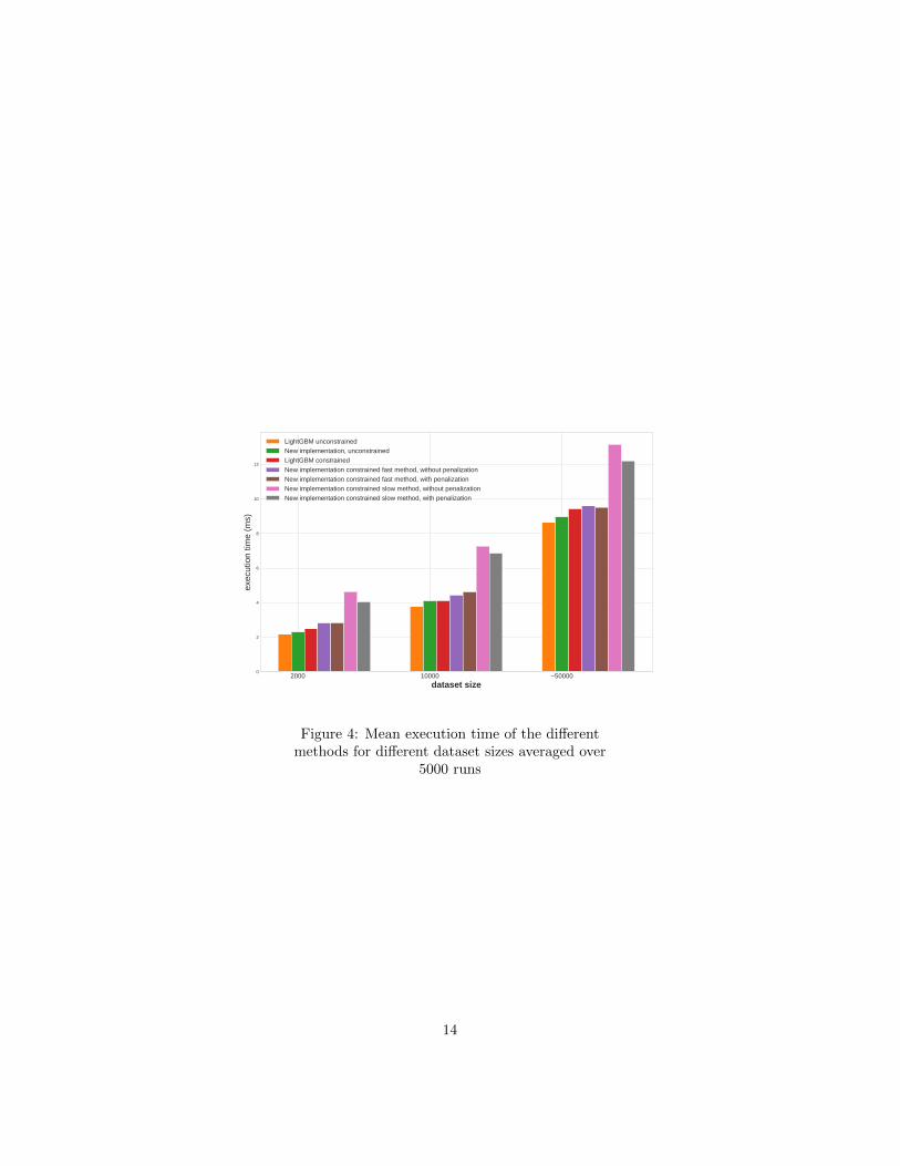
1.5 Computation time for each method

On figure 4, we report the computational cost for each method. We measuredit using the timeit module in Python (so the results are not very precise, asthe standard deviation can be as high as 1ms). These statistics were createdusing either 2000, 10000, or close to 50000 random entries. The execution timeswere measured over 1 boosting iteration, using a maximum depth of 10 and amaximum number of leaves of 40, and the trees were filled with the maximumnumber of leaves every time. The results are averaged across 5000 runs.

Even though these results are a bit noisy, we can draw very useful insightsfrom them. Overall, whether we are using LightGBM or our new fast method,the difference in computational costs is not very significant. The slow method is,however, much slower than the current LightGBM. Nonetheless, the differencemitigates when the dataset is bigger and building histogram is a more importanttask.

1.6 Plots of the first trees generated by each method

On figures 5, 6, 7, 8, 9 and 10, we plotted the first trees generated by ourdifferent methods to see how they would differ. Here are a few things to noticeto understand the tree visualizations,

5

• The trees are all compared to the unconstrained tree. A red leaf meansthat the leaf does not appear in the unconstrained tree. A red nodemeans that the node does not appear in the unconstrained tree (either thesplitting feature is different or the threshold is different, or the parent ofthe node is different). A red gain means that the gain for the same nodein the unconstrained tree is different;

• A green node means that the node is monotonically increasing;

• Blue numbers on the nodes show the order in which the nodes have beensplit.

Here are a few observations coming from the comparison of the trees,

• As anticipated, the monotone features are extremely important, becausethey appear in many nodes in the first trees;

• Up to a certain point (until the first monotone split), all trees are similarto the unconstrained tree;

• For the penalized method, we can indeed see that no monotone split hap-pened in the first levels of the tree;

• The outputs of the first tree are all negative because the dataset is imbal-anced and there are a lot more 0’s than 1’s;

• The trees get even more different as the algorithms keep running;

• Gains for the unconstrained method seem generally greater than for therest of the methods, which makes sense. Also, the unconstrained methodhas more leaves on this example, which is also coherent.

2 Explanations of the new methods

2.1 New ways of constraining trees

We developed 2 new ways of constraining trees. Both yield better results thanthe current LightGBM constraining method. One of the method is about as fastas the current LightGBM. The other method is much slower (can be as muchas twice as slow in extreme worst case scenarii), but is also more accurate. Inthis section, we will present both.

Both methods originally stem from the observation that the current Light-GBM constraining method is over-constraining the trees. In our methods, whenwe make a monotone split, instead of imposing constraints on both childrenthat make the outputs of all their descendants mutually exclusive, as LightGBMcurrently does by setting a mid point, we chose to set up only the necessary con-straints every time so that the next split would not break the monotone rules.

6

More precisely, this means that if the split is monotonically increasing, then theleft child gets the right output as a maximum constraint, and the right childgets the left output as a minimum constraint. However, is the split is mono-tonically decreasing, then it means that the left child gets the right output asa minimum constraint and the right child gets the left output as a maximumconstraint constraint.

Then, when we make any split (monotone or not) in a branch having amonotone node as a parent somewhere, after making the split, we need to checkthat the new outputs are not violating any constraint on other leaves of thetree. The general idea is that we should start from the node where a split wasjust made, go up the tree, and every time a monotone node is encountered,we should go down in the opposite branch and check that the constraints andthe new outputs from the new split are compatible. If they are not, then theconstraints need to be updated. Therefore making a split in a branch can verywell update the constraints of other leaves in another branch.

2.1.1 The computationally efficient way of constraining trees

In this method, only one minimum constraint and one maximum constraintneed to be stored for each leaf. A constraint is computed as the extremum ofall constraints applied sequentially on a leaf during the construction of the tree.That makes the constraints very easy to compute, because when a constraintof a leaf has to be updated, it can be done only by performing a minimumor a maximum. This method is better than the current LightGBM because itdoesn’t create ”gaps” between leaves, and it is still efficient, because the onlyadditional thing we need is going through the tree and recomputing some splitsometimes, but usually not that much (especially when we compare it to thetime spent building histograms).

2.1.2 The slower yet more accurate way of constraining the trees

This method is based on the same principle except that for each leaf, for eachfeature, for each threshold, we are going to store one minimum and one maxi-mum constraints. By doing that, we are going to have many different constraintsfor every leaf (at most number of features times number of thresholds times 2for minimum and maximum constraints per leaf, but usually, it is quite a lotless than that). Then when a split has to be made with respect to a feature,we can have different left and right constraints for the children depending onwhere the constraints were applied on the original leaf. Additionally, when asplit is made, and we start updating the constraints of other leaves, we takeinto account the fact that the split may very well have ”unconstrained” someleaves (as well as constrained others). By doing that we are sometimes able tosplit leaves that would not be splittable using the previous methods. Moreover,since we compute the exact constraints needed everywhere at every iteration ofbuilding the trees, we are not over-constraining any leaf, and therefore trees can

7

get much more accurate. However, when using this method, we need to storelots of constraints that are going to be updated very often. Furthermore, whena leaf is ”unconstrained”, then all the constraints need to be computed fromthe beginning (otherwise we would need to store which leaves the constraintscome from, and keep them sorted, which, in our opinion, would not be better).Because of that, this method is quite a lot slower, even though we tried toimplement many optimizations so that it would remain tractable.

2.2 Theoretical example

On figure 11, we imagined a simple situation demonstrating the improvementsof our methods. Let’s imagine that we have a regression problem, with the databeing represented on figure 11a. The only constraint is that the output hasto be monotonically increasing horizontally. The true labels of the points aregiven on the right of figure 11a. On figure 11a, we take it as given that the firstsplit is the same with all methods and that it yields the values written on thegraph. On figure 11b, we assume that the second split is again the same withall methods and that it yields the values written on the graph. The 3 followingfigures depict what would happen for the following split with each method.

• On figure 11c, with LightGBM, since the values on the graph from figure11a were 0.3 and 0.6, the mid point is 0.45. Therefore, the blue dots areupper bounded and labelled as 0.45.

• On figure 11d, with the fast method, once the first split is made, the leafon the left is given an upper bound of 0.6. Once the second split is made,every leaf on the left is given an upper bound of 0.5. Therefore, the bluedots are labelled as 0.5

• On figure 11e, with the slow method, once the first split is made, the leafon the left is given an upper bound of 0.6. Once the second split is made,the top part of the left leaf is given an upper bound of 0.5, and the lowerpart of the left leaf is given an upper bound of 0.8. Therefore, the bluedots are labelled as 0.7, their true value.

We can therefore see that our methods are better at this specific regressionproblem, the slow method achieving optimal results with only one tree. Similarexamples happen very often both in regression and classification tasks, whenbuilding trees. Therefore, our methods should consistently yield better resultsthan the current LightGBM implementation.

2.3 A heuristic penalty for monotone splits

2.3.1 Why penalizing monotone splits is a good idea

The main drawback of adding monotone constraints to a tree is that it may endup over-constraining the tree because of the greediness of the tree splitting al-gorithm, and therefore loose in predictive power. By building a tree in a greedy

8

fashion, we don’t know how much the constraints of monotone splits are goingto affect the following nodes (it may reduce the gain of the children by a lot).For our new methods, we don’t know either by how by much a new split is go-ing to constrain other surrounding leaves and their future children (in the eventthat the leaf we are splitting is part of a branch growing from a monotone node).

When using our new method, even though it already yields good results aswe will see in section 1, both these effect happen in almost any tree with rea-sonable depth when making at least one monotone split. However, we do notquantify or take into account any of these 2 drawbacks at all in the algorithm.Yet they can be huge at the first levels of the trees, because the constraintsare going to affect most of the leaves. Therefore, amongst other things, we arevery likely to overestimate the gain generated by splitting a leaf on a monotonefeature; especially early in the trees, where the constraints are going to impactmany leaves.

Unfortunately, this reduction of gain can’t be computed greedily. Indeed, wewould need to know what is going to happen after to quantify it (or we couldtry to predict it but that is not an easy task either). However, we were ableto develop a simple heuristic that improves the results, by penalizing monotonesplits early when building trees.

The general idea of the heuristic is that we are likely to not want to make amonotone split in the first levels of a tree because this is going to constrain toomany leaves. Then, generally, the deeper we go, the more inclined to monotonespits we are. This is a very general rule than can have many exceptions, but webelieve it is true more often than not. Therefore, we designed a penalty functionthat is a function of depth, that will multiply the gain of monotone splits at agiven depth. It is parametrised by only one parameter that we will call γ herefor simplicity, and that allows monotone splits to be penalized the higher theyappear in a tree.

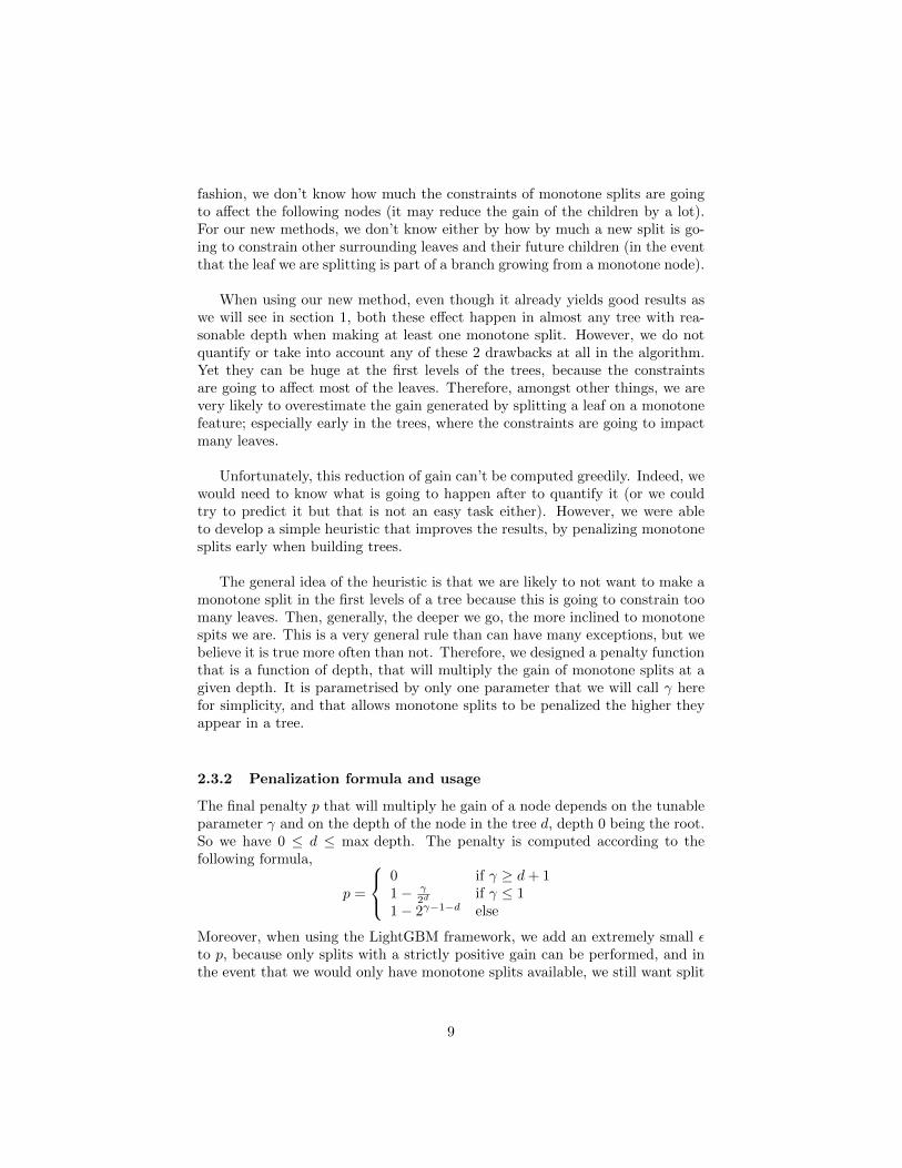
2.3.2 Penalization formula and usage

The final penalty p that will multiply he gain of a node depends on the tunableparameter γ and on the depth of the node in the tree d, depth 0 being the root.So we have 0 ≤ d ≤ max depth. The penalty is computed according to thefollowing formula,

p =

0 if γ ≥ d+ 11− γ

2dif γ ≤ 1

1− 2γ−1−d else

Moreover, when using the LightGBM framework, we add an extremely small εto p, because only splits with a strictly positive gain can be performed, and inthe event that we would only have monotone splits available, we still want split

9

one of them.

On figure 12 we plotted what the penalty looks like for different penalizationparameters, as a function of depth. There are some important things to mentionabout this penalty function:

• When γ = 0, then there is no penalty at all;

• When γ ∈ [0; 1], then we gradually penalize all depths, and the closer to1 they are, the more they are penalized;

• When γ ∈ [1; 2], then the penalty for the first level is 0 (we prohibit anymonotone split on this level), and we keep gradually penalizing monotonesplits at all depths, and the closer to depth 2 they are, the more they arepenalized;

• When γ ∈ [2; 3], then the penalty for the first two levels is 0 (we prohibitany monotone split on these levels), and we keep gradually penalizingmonotone splits at all depths, and the closer to depth 3 they are, themore they are penalized;

• ...

Therefore, the parameter γ is a very intuitive parameter that shouldn’t confusethe end user.

2.3.3 Penalization vs. depth plot

On figure 12, we plot the penalty factor that will multiply the gain of monotonesplits, for different depths and penalization parameters.

10

3 Conclusion

In this report, we propose two new methods to enforce monotonic constraintsin regression and classification trees, as well as a heuristic to improve the re-sults. During our tests, we found that our new methods consistently achievebetter results than the current LightGBM constraining method. Our fastestmethod does not generate significant additional computational cost comparedto the current LightGBM. Therefore, we believe that our work should replacethe current LightGBM implementation. Finally, as mentioned previously, ourwork is not LightGBM-specific and could be implemented in any regression orclassification tree.

11

Figure 2: Loss and metrics vs. number of iterationsrelative to the constrained LightGBM baseline, for

all methods, on the train and test sets

12

Figure 2: Loss and metrics vs. number of iterationsrelative to the constrained LightGBM baseline, for

all methods, on the train and test sets

0 0.5 1 1.5 2 2.5 3 3.5 4 4.5 5

penalization parameter

1020

3040

5075

100

150

200

300

400

500

num

ber 

of tr

ees

­0.00% 0.17% 0.26% 0.31% 0.33% 0.15% 0.07% ­1.12% ­1.54% ­2.16% ­4.23%

­0.00% 0.43% 0.44% 0.45% 0.41% 0.23% ­0.04% ­1.25% ­1.70% ­2.46% ­6.73%

­0.00% 0.46% 0.51% 0.62% 0.55% 0.47% 0.23% ­0.69% ­1.20% ­1.98% ­7.97%

­0.00% 0.51% 0.62% 0.66% 0.68% 0.52% 0.39% ­0.41% ­0.91% ­1.67% ­8.87%

­0.00% 0.67% 0.75% 0.78% 0.81% 0.70% 0.57% ­0.07% ­0.64% ­1.36% ­9.32%

­0.00% 0.50% 0.64% 0.71% 0.70% 0.65% 0.63% 0.21% ­0.34% ­0.95% ­10.50%

­0.00% 0.42% 0.56% 0.63% 0.61% 0.55% 0.57% 0.33% ­0.07% ­0.57% ­11.04%

­0.00% 0.35% 0.46% 0.50% 0.53% 0.49% 0.48% 0.40% 0.12% ­0.20% ­11.60%

­0.00% 0.33% 0.45% 0.50% 0.54% 0.50% 0.46% 0.42% 0.15% ­0.06% ­11.81%

­0.00% 0.34% 0.40% 0.43% 0.51% 0.42% 0.43% 0.35% 0.01% ­0.09% ­12.30%

­0.00% 0.28% 0.38% 0.45% 0.36% 0.38% 0.31% 0.26% ­0.11% ­0.17% ­12.66%

­0.00% 0.18% 0.38% 0.41% 0.41% 0.28% 0.27% 0.15% ­0.20% ­0.25% ­12.91%

Loss reduction generated by the penalized splits relative to the unpenalized splits, on the train set

­2%

­2%

­1%

0%

1%

Figure 3: Relative loss reduction for penalizedmonotone splits, compared to unpenalized splits, for

different penalization parameters, fot the fastmethod

13

2000 10000 ~50000dataset size

0

2

4

6

8

10

12

execution tim

e (m

s)

LightGBM unconstrainedNew implementation, unconstrainedLightGBM constrainedNew implementation constrained fast method, without penalizationNew implementation constrained fast method, with penalizationNew implementation constrained slow method, without penalizationNew implementation constrained slow method, with penalization

Figure 4: Mean execution time of the differentmethods for different dataset sizes averaged over

5000 runs

14

Figure 5: First two trees generated by theunconstrained method15

Figure 6: First two trees generated by the baselineLightGBM method

16

Figure 7: First two trees generated by our new slowmethod, with no penalization

17

Figure 8: First two trees generated by our new slowmethod, with a penalization parameter of 2

18

Figure 9: First two trees generated by our new fastmethod, with no penalization

19

Figure 10: First two trees generated by our new fastmethod, with a penalization parameter of 2

20

True values

0.7

0.5

0.8

0.2

monotone increasing

unconstrained

0.3 0.6

(a) First split

0.3

0.5

0.8

(b) Second split

0.2

0.45

0.5

0.8

(c) Third split LightGBM

0.2

0.5

0.5

0.8

(d) Third split fast method

0.7

0.2 0.5

0.8

(e) Third split slow method

Figure 11: Theoretical example of the behavior of the different constrainingmethods

21

0 1 2 3 4 5

Depth

0.0

0.2

0.4

0.6

0.8

1.0

Pen

alization factor

Penalization of monotone splits vs. depth for different values of γ

Penalization parameter=0.0Penalization parameter=0.25Penalization parameter=0.5Penalization parameter=0.75Penalization parameter=1.0Penalization parameter=1.25Penalization parameter=1.5Penalization parameter=1.75Penalization parameter=2.0Penalization parameter=2.25Penalization parameter=2.5Penalization parameter=2.75Penalization parameter=3.0Penalization parameter=3.25Penalization parameter=3.5Penalization parameter=3.75Penalization parameter=4.0Penalization parameter=4.25Penalization parameter=4.5Penalization parameter=4.75Penalization parameter=5.0

Figure 12: Penalty function for differentpenalization parameters

22