c©2017 IEEE. Personal use of this material is permitted. Permission from IEEE must be obtained for all other uses, in anycurrent or future media, including reprinting/republishing this material for advertising or promotional purposes, creating newcollective works, for resale or redistribution to servers or lists, or reuse of any copyrighted component of this work in otherworks.

This is a preprint version. The final version of this paper is available at http://ieeexplore.ieee.org/document/8280935/(DOI:10.1109/SSCI.2017.8280935).

.

A Benchmark Environment Motivated byIndustrial Control Problems

Daniel Hein∗†§, Stefan Depeweg∗†§, Michel Tokic†, Steffen Udluft†,Alexander Hentschel‡, Thomas A. Runkler∗† and Volkmar Sterzing†

∗Technische Universitat Munchen, Department of Informatics, Boltzmannstr. 3, 85748 Garching, Germany†Siemens AG, Corporate Technology, Otto-Hahn-Ring 6, 81739 Munich, Germany

‡AxiomZen, 980 Howe St #350, Vancouver, BC V6Z 1N9, Canada

Abstract—In the research area of reinforcement learning (RL),frequently novel and promising methods are developed andintroduced to the RL community. However, although manyresearchers are keen to apply their methods on real-world prob-lems, implementing such methods in real industry environmentsoften is a frustrating and tedious process. Generally, academicresearch groups have only limited access to real industrial dataand applications. For this reason, new methods are usuallydeveloped, evaluated and compared by using artificial softwarebenchmarks. On one hand, these benchmarks are designed toprovide interpretable RL training scenarios and detailed insightinto the learning process of the method on hand. On theother hand, they usually do not share much similarity withindustrial real-world applications. For this reason we used ourindustry experience to design a benchmark which bridges the gapbetween freely available, documented, and motivated artificialbenchmarks and properties of real industrial problems. Theresulting industrial benchmark (IB) has been made publiclyavailable to the RL community by publishing its Java and Pythoncode, including an OpenAI Gym wrapper, on Github. In thispaper we motivate and describe in detail the IB’s dynamics andidentify prototypic experimental settings that capture commonsituations in real-world industry control problems.

I. INTRODUCTION

Applying reinforcement learning (RL) methods to industrialsystems, such as in process industry like steel processing [1],pulp and paper processing [2], and car manufacturing [3],or power generation with gas or wind turbines [4], [5], isan exciting area of research. The hope is that an intelligentagent will provide greater energy efficiency and, desirably, lesspolluting emissions. However, the learning process also entailsa significant amount of risk: we do not know beforehand howa particular learning algorithm will behave, and with complexand expensive systems like these, experiments can be costly.

§ Equal contributions.

Therefore, there is high demand in having simulations thatshare some of the properties that can be observed in theseindustrial systems.

The existing simulation benchmarks have lead to greatadvancements in the field of RL. Traditionally simple dy-namical systems like pendulum dynamics are studied, whereasnowadays the focus has shifted towards more complex sim-ulators, such as video game environments [6]. Also in thefield of robotics very sophisticated simulation environmentsexist, on which new learning algorithms can be tested [7], [8].The existence of such benchmarks has played a vital role inpushing the frontier in this domain of science.

For industrial control, however, such a test bed is lacking.In these systems we observe a combination of propertiesthat usually are not present in existing benchmarks, such ashigh dimensionality combined with complex heteroscedasticstochastic behavior. Furthermore, in industrial control differentexperimental settings are of relevance, for instance, the focus isusually less on exploration, and more on batch RL settings [9].

To this end, we recently developed the industrial bench-mark (IB), an open source software benchmark1, with bothJava and Python implementations, including an OpenAI Gymwrapper, available. Previously, this benchmark has alreadybeen used to demonstrate the performance of a particle swarmbased RL policy approach [10]. The contribution of thispaper lies in presenting the complete benchmark frameworkas well as mathematical details, accompanied by illustrationsand motivations for several design decisions. The IB aimsat being realistic in the sense that it includes a variety ofaspects that we found to be vital in industrial applicationslike optimization and control of gas and wind turbines. It isnot designed to be an approximation of any real system, but

1Java/Python source code: http://github.com/siemens/industrialbenchmark

arX

iv:1

709.

0948

0v2

[cs

.AI]

6 F

eb 2

018

to pose the same hardness and complexity. Nevertheless, theprocess of searching for an optimal action policy on the IB issupposed to resemble the task of finding optimal valve settingsfor gas turbines or optimal pitch angles and rotor speeds forwind turbines.

The state and action spaces of the IB are continuous andhigh-dimensional, with a large part of the state being latent tothe observer. The dynamical behavior includes heteroscedasticnoise and a delayed reward signal that is composed of multipleobjectives. The IB is designed such that the optimal policy willnot approach a fixed operation point in the three steerings. Allof these design choices were driven by our experience withindustrial challenges.

This paper has three key contributions: in Section II, wewill embed the IB in the landscape of existing benchmarksand show that it possesses a combination of properties otherbenchmarks do not provide, which makes it a useful additionas a test bed for RL. In Section III we will give a detaileddescription of the dynamics of the benchmark. Our thirdcontribution, described in Section IV, is to define prototypeexperimental setups that we find relevant for industrial control.Our goal is to encourage other researchers to study scenarioscommon in real-world situations.

II. PLACEMENT OF THE INDUSTRIAL BENCHMARK IN THERL BENCHMARK DOMAIN

In the RL community numerous benchmark suits exist,on which novel algorithms can be evaluated. For researchin industrial control we are interested in a particular set ofproperties, such as stochastic dynamics with high dimensionalcontinuous state and action spaces. We argue that only fewfreely available benchmarks exist fulfilling these properties,thereby making our contribution, the IB, a useful addition. Tothat end, we want to briefly review existing benchmarks inRL.

Classic control problems in RL literature [11], such as thecart-pole balancing and mountain car problems, usually havelow dimensional state and action spaces and deterministicdynamics. In the field of robotics more complex and high-dimensional environments exist with a focus on robot locomo-tion, such as the MuJoCo environment [7], [8]. Other examplesare helicopter flight2 [12] or learning to ride a bicycle [13].These systems, while complex, usually have deterministicdynamics or only limited observation noise.

Utilizing games as RL benchmarks recently brought promis-ing results of deep RL into the focus of a broad audience.Famous examples include learning to play Atari games3 [6],[14] based on raw pixels, achieving above-human performanceplaying Ms. Pac-Man [15], and beating human experts in thegame of Go [16]. In these examples, however, the action spaceis discrete and insights from learning to play a game may nottranslate to learning to control an industrial system like gas orwind turbines.

2https://sites.google.com/site/rlcompetition2014/domains/helicopter3https://github.com/mgbellemare/Arcade-Learning-Environment

Stat

edi

men

sion

s

Stochasticity

• IB

• Helicopter

• MuJoCo

• Cart-pole• Bicycle

• Mountain Car• Wet Chicken

Fig. 1. Qualitative comparison of different RL benchmarks with continuousactions. The state space of the wet chicken 2D benchmark [17] is rather low,but it is highly stochastic which makes it a challenging RL problem. Cart-poleand mountain car are deterministic benchmarks with few state dimensionsand only a single action variable. The bicycle benchmark introduces somenoise to simulate imperfect balance. The helicopter software simulation hasa 12-dimensional state space and a 4-dimensional continuous action space.Stochasticity is introduced to simulate wind effects on the helicopter. Thestate space of the IB is high, since multiple past observations have to be takeninto account to approximate the true underlying Markov state. Stochasticityis not only introduced by adding noise on different observations, but also bystochastic state transitions on hidden variables.

In Figure 1 we give a qualitative overview on the placementof the proposed IB with respect to other RL benchmarks forcontinuous control. Here, we focus on stochasticity and dimen-sionality of the benchmarks at hand. Note that by stochasticitywe do not only refer to the signal to noise ratio, but also to thestructural complexity of the noise, such as heteroscedasticityor multimodality. We conclude that the IB is a useful additionto the set of existing RL benchmarks. In particular, Figure 1illustrates that the combination of high dimensionality andcomplex stochasticity appears to be novel compared to existingenvironments. In the following section, a detailed descriptionand motivation for the applied IB dynamics is presented.

III. DETAILED DESCRIPTION

At any time step t the RL agent can influence the environ-ment, i.e., the IB, via actions at that are three dimensionalvectors in [−1, 1]3. Each action can be interpreted as threeproposed changes to the three observable state variables calledcurrent steerings. Those current steerings are named velocityv, gain g, and shift h. Each of those is limited to [0, 100] asfollows:

at = (∆vt,∆gt,∆ht), (1)

vt+1 = max(0,min(100, vt + dv∆vt)), (2)gt+1 = max(0,min(100, gt + dg∆gt)), (3)ht+1 = max(0,min(100, ht + dh∆st)), (4)

with scaling factors dv = 1, dg = 10, and dh = 5.75. The stepsize for changing shift is calculated as dh = 20 sin(150)/0.9 ≈5.75.

After applying action at, the environment transitions to thenext time step t + 1 in which it enters internal state st+1.State st and successor state st+1 are the Markovian states ofthe environment that are only partially observable to the agent.

An observable variable of the IB, setpoint p, influencesthe dynamical behavior of the environment but can neverbe changed by actions. An analogy to such a setpoint is,for example, the demanded load in a power plant or thewind speed actuating a wind turbine. As we will see inthe upcoming description, different values of setpoint p willinduce significant changes to the dynamics and stochasticityof the benchmark. The IB has two modes of operation: a)fixing the setpoint to a value p = const, thereby acting as ahyperparameter or b) as a time-varying external driver, makingthe dynamics become highly non-stationary. We give a detaileddescription of setting b) in Subsection III-D.

The set of observable state variables is completed by tworeward relevant variables, consumption ct and fatigue ft. In thegeneral RL setting a reward rt+1 for each transition t→ t+1from state st via action at to the successor state st+1 is drawnfrom a probability distribution depending on st, at, and st+1.In the IB, the reward is given by a deterministic function ofthe successor state rt+1 = r(st+1), i.e.,

rt+1 = −ct+1 − 3ft+1. (5)

In the real-world tasks that motivated the IB, the rewardfunction has always been known explicitly. In some cases ititself was subject to optimization and had to be adjusted toproperly express the optimization goal. For the IB we thereforeassume that the reward function is known and all variablesinfluencing it are observable.

Thus the observation vector ot at time t comprises currentvalues of the set of observable state variables, which is a subsetof all the variables of Markovian state st, i.e.,

1) the current steerings, velocity vt, gain gt, and shift ht,2) the external driver, setpoint pt,3) and the reward relevant variables consumption ct and

fatigue ft.Appendix A gives a complete overview on the IB’s state space.

The data base for learning comprises tuples(ot, at, ot+1, rt). The agent is allowed to use all previousobservation vectors and actions to estimate the Markovianstate st.

The dynamics can be decomposed into three different sub-dynamics named operational cost, mis-calibration, and fatigue.

A. Dynamics of operational cost

The sub-dynamics of operational cost are influenced bythe external driver setpoint p and two of the three steerings,velocity v and gain g. The current operational cost θt iscalculated as

θt = exp

(2pt + 4vt + 2.5gt

100

). (6)

The observation of θt is delayed and blurred by the followingconvolution:

θct =

1

9θt−5 +

2

9θt−6 +

3

9θt−7 +

2

9θt−8 +

1

9θt−9. (7)

The convoluted operational cost θct cannot be observed di-rectly, instead it is modified by the second sub-dynamic,called mis-calibration, and finally subject to observation noise.The motivation for this dynamical behavior is that it is non-linear, it depends on more than one influence, and it isdelayed and blurred. All those effects have been observedin industrial applications, like the heating process observableduring combustion. In Figure 4b we give an example trajectoryof the convolution process over a rollout of 200 time steps.The delayed and blurred relations between operational cost θtand the convoluted costs θct are clearly visible.

B. Dynamics of mis-calibration

The sub-dynamics of mis-calibration are influenced byexternal driver setpoint p and steering shift h. The goal isto reward an agent to oscillate in h in a pre-defined frequencyaround a specific operation point determined by setpoint p.Thereby, the reward topology is inspired by an example fromquantum physics, namely Goldstone’s ”Mexican hat” potential.

In the first step, setpoint p and shift h are combined to aneffective shift he calculated by:

he = max

(−1.5,min

(1.5,

h

20− p

50− 1.5

)). (8)

Effective shift influences three latent variables, which aredomain δ, response ψ, and direction φ. Domain δ can enter twodiscrete states, which are negative and positive, representedby integer values −1 and +1, respectively. Response ψ canenter two discrete states, which are disadvantageous andadvantageous, represented by integer values −1, and +1,respectively. Direction φ ∈ {−6,−5, . . . , 6} is a discrete indexvariable, yielding the position of the current optima in the mis-calibration penalty space.

Figure 2 is a visualization of the mis-calibration dynamicsintroduced in equation form in the following paragraphs. Ineach time step t → t + 1 the mis-calibration dynamics aretransitioned starting with δ and ψ as follows:

δt+1 =

{δt if |he| ≤ zsgn(he) else,

(9)

ψt+1 =

{1 if δt 6= δt+1

ψt else,(10)

where safe zone z (area in the center of Figure 2) is calculatedusing z = sin(π · 15/180)/2 ≈ 0.1309. Note that the policyitself is allowed to decide when to leave the safe zone.

In the next step, direction index φ is updated accordingly:

φt+1 = φt + ∆φt+1,with (11)

he

φ

1.5

1.0

0.0

-1.0

-1.5-6 -5 -4 -3 -2 -1 0 1 2 3 4 5 6

decreasesφ

increasesφ

constantφ

constantφ

reset

decreasesφincreasesφsafe zone−z

+z

δ = +1

δ = −1

positive domain

negative domain

advantageous response…………..ψ = +1

disadvantageous response…………..

ψ = +1

disadvantageous response…………..ψ = −1

advantageous response…………..

ψ = −1

Fig. 2. Visual description of the mis-calibration dynamics. Blue colorrepresents areas of low penalty (-1.00), while yellow color represents areasof high penalty (1.23). If the policy keeps he in the so-called safe zone, φis driven towards 0 stepwise. When φ = 0 is reached the mis-calibrationdynamics are reset, i.e., domain δ = 1 and response ψ = 1. The policy isallowed to start the rotation cycle at any time by leaving the safe zone andentering the positive or the negative domain. Consider positive domain δ = 1:After initially leaving the safe zone, response is in the state advantageous, i.e.,φ is increased stepwise. The upper right area is a reversal point for φ. As soonas φ = 6, response switches from advantageous ψ = 1 to disadvantageousψ = −1. In the subsequent time steps φ is decreased until either the policybrings he back to the safe zone or φ reaches the left boundary at -6. If thelatter occurs, phi is kept constant at -6, i.e., the policy yields a high penaltyin each time step. Since the mis-calibration dynamics are symmetric around(φ, he) = (0, 0), opposite dynamics are applied in the negative domain atthe lower part of the plot.

∆φt+1 =

− sgn(φt) if |he| ≤ z0 if |he| > z ∧ φt = −6δt+1

ψt+1 · sgn(he) else.(12)

The first option realizes the return of φ if the policy returnsinto the safe zone. The second option stops the rotation ifφ reaches the opposite domain bound (upper left and lowerright area in Figure 2). The third option implements the cyclicmovement of φ depending on response ψ and the direction ofeffective shift he.

If, after this update, the absolute value of direction index φreaches or exceeds the predefined maximum index of 6 (upperright and lower left area in Figure 2), response enters statedisadvantageous and index φ is turned towards 0.

ˆψt+1 =

{−1 if |φt+1| ≥ 6

ψt+1 else.(13)

φt+1 =

{12− ((φt+1 + 24) mod 24) if |φt+1| ≥ 6

φt+1 else.(14)

In the final step of the mis-calibration state transition, it ischecked if effective shift he has returned to safe zone z whileat the same time direction index φ has completed a full cycle(reset area in the center of Figure 2). If this is the case, domainδ and response ψ are reset to their initial states positive andadvantageous, respectively:

δt+1 =

{1 if φt+1 = 0 ∧ |he| ≤ zδt+1 else.

(15)

ψt+1 =

{1 if φt+1 = 0 ∧ |he| ≤ zˆψt+1 else.

(16)

Note that in this state the policy can again decide to start anew cycle (positive or negative direction) or to remain in stateφ = 0.

The penalty landscape of mis-calibration is computed asfollows. Based on the current value of φ, the penalty functionm(φ, he) computes the performance of maintaining shift in thebeneficial area. The penalty function m is defined as a linearlybiased Goldstone potential computed by

m = −αω2 + βω4 + κρsω. (17)

The definition of radius ω can be found in Appendix B. Fromdirection index φ the sine of direction angle ρ is calculated asfollows:

ρs = sin( π

12φ). (18)

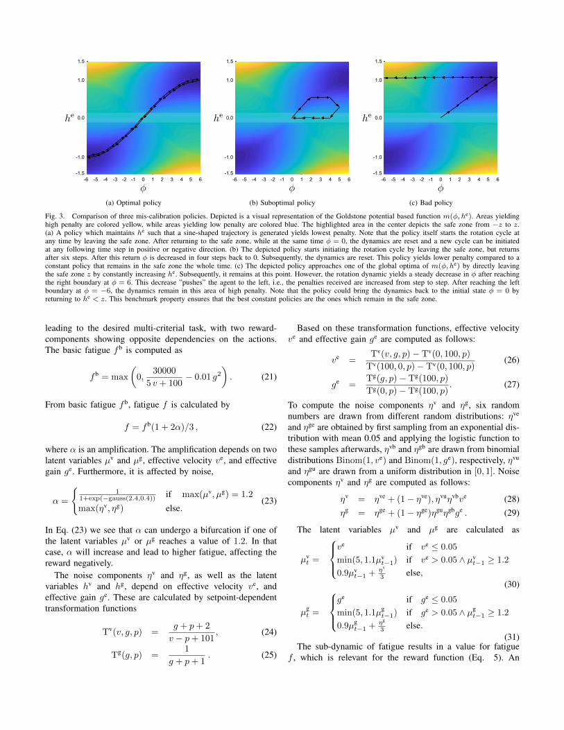
Note that this sine function represents the optimal policy forthe mis-calibration dynamics. Exemplary policy trajectoriesthrough the penalty landscape of mis-calibration are depictedand described in Figure 3.

The resulting mis-calibration mt is added to the convolutedoperational cost θc

t , giving ct,

ct = θct + 25mt. (19)

Before being observable as consumption ct, the modifiedoperational cost ct is subject to heteroscedastic observationnoise

ct = ct + gauss(0, 1 + 0.02 ct) , (20)

i.e., a Gaussian noise with zero mean and a standard deviationof σ = 1+0.02 ct. In Figure 4c we show in an example rolloutof 200 steps how both convoluted operational cost θct and mis-calibration mt affect consumption ct.

C. Dynamics of fatigue

The sub-dynamics of fatigue are influenced by the samevariables as the sub-dynamics of operational cost, i.e., setpointp, velocity v, and gain g. The IB is designed in such away that, when changing the steerings velocity v and gaing as to reduce the operational cost, fatigue will be increased,

he

φ

1.5

1.0

0.0

-1.0

-1.5-6 -5 -4 -3 -2 -1 0 1 2 3 4 5 6

(a) Optimal policy

he

φ

1.5

1.0

0.0

-1.0

-1.5-6 -5 -4 -3 -2 -1 0 1 2 3 4 5 6

(b) Suboptimal policy

he

φ

1.5

1.0

0.0

-1.0

-1.5-6 -5 -4 -3 -2 -1 0 1 2 3 4 5 6

(c) Bad policy

Fig. 3. Comparison of three mis-calibration policies. Depicted is a visual representation of the Goldstone potential based function m(φ, he). Areas yieldinghigh penalty are colored yellow, while areas yielding low penalty are colored blue. The highlighted area in the center depicts the safe zone from −z to z.(a) A policy which maintains he such that a sine-shaped trajectory is generated yields lowest penalty. Note that the policy itself starts the rotation cycle atany time by leaving the safe zone. After returning to the safe zone, while at the same time φ = 0, the dynamics are reset and a new cycle can be initiatedat any following time step in positive or negative direction. (b) The depicted policy starts initiating the rotation cycle by leaving the safe zone, but returnsafter six steps. After this return φ is decreased in four steps back to 0. Subsequently, the dynamics are reset. This policy yields lower penalty compared to aconstant policy that remains in the safe zone the whole time. (c) The depicted policy approaches one of the global optima of m(φ, he) by directly leavingthe safe zone z by constantly increasing he. Subsequently, it remains at this point. However, the rotation dynamic yields a steady decrease in φ after reachingthe right boundary at φ = 6. This decrease ”pushes” the agent to the left, i.e., the penalties received are increased from step to step. After reaching the leftboundary at φ = −6, the dynamics remain in this area of high penalty. Note that the policy could bring the dynamics back to the initial state φ = 0 byreturning to he < z. This benchmark property ensures that the best constant policies are the ones which remain in the safe zone.

leading to the desired multi-criterial task, with two reward-components showing opposite dependencies on the actions.The basic fatigue f b is computed as

f b = max

(0,

30000

5 v + 100− 0.01 g2

). (21)

From basic fatigue f b, fatigue f is calculated by

f = f b(1 + 2α)/3 , (22)

where α is an amplification. The amplification depends on twolatent variables µv and µg, effective velocity ve, and effectivegain ge. Furthermore, it is affected by noise,

α =

{1

1+exp(−gauss(2.4,0.4)) if max(µv, µg) = 1.2

max(ηv, ηg) else.(23)

In Eq. (23) we see that α can undergo a bifurcation if one ofthe latent variables µv or µg reaches a value of 1.2. In thatcase, α will increase and lead to higher fatigue, affecting thereward negatively.

The noise components ηv and ηg, as well as the latentvariables hv and hg, depend on effective velocity ve, andeffective gain ge. These are calculated by setpoint-dependenttransformation functions

Tv(v, g, p) =g + p+ 2

v − p+ 101, (24)

Tg(g, p) =1

g + p+ 1. (25)

Based on these transformation functions, effective velocityve and effective gain ge are computed as follows:

ve =Tv(v, g, p)− Tv(0, 100, p)

Tv(100, 0, p)− Tv(0, 100, p)(26)

ge =Tg(g, p)− Tg(100, p)

Tg(0, p)− Tg(100, p). (27)

To compute the noise components ηv and ηg, six randomnumbers are drawn from different random distributions: ηve

and ηge are obtained by first sampling from an exponential dis-tribution with mean 0.05 and applying the logistic function tothese samples afterwards, ηvb and ηgb are drawn from binomialdistributions Binom(1, ve) and Binom(1, ge), respectively, ηvu

and ηgu are drawn from a uniform distribution in [0, 1]. Noisecomponents ηv and ηg are computed as follows:

ηv = ηve + (1− ηve), ηvuηvbve (28)ηg = ηge + (1− ηge)ηguηgbge . (29)

The latent variables µv and µg are calculated as

µvt =

ve if ve ≤ 0.05

min(5, 1.1µvt−1) if ve > 0.05 ∧ µv

t−1 ≥ 1.2

0.9µvt−1 + ηv

3 else,(30)

µgt =

ge if ge ≤ 0.05

min(5, 1.1µgt−1) if ge > 0.05 ∧ µg

t−1 ≥ 1.2

0.9µgt−1 + ηg

3 else.(31)

The sub-dynamic of fatigue results in a value for fatiguef , which is relevant for the reward function (Eq. 5). An

0 25 50 75 100 125 150 175 200t

30

40

50

60

70

80

90

100ft

ft

µgt

0

1

2

3

4

5

µg t

(a) Fatigue dynamics

0 25 50 75 100 125 150 175 200t

20

30

40

50

60

70

Op

erat

iona

lC

ost

θtθct

(b) Operational cost

0 25 50 75 100 125 150 175 200t

−20

0

20

40

60

80

100

120

140

Con

sum

ptio

n

25mt

θct

ct

(c) Consumption dynamics

0 25 50 75 100 125 150 175 200t

50

100

150

200

250

300

350

−rt

ct3ft−rt

(d) Reward dynamics

Fig. 4. Visualization of relevant variables of the IB in a rollout using random actions over 200 time steps. (a): Shown are latent variable µg and fatigue f .As seen in Eq. (23), the latent variable can lead to a bifurcation of the dynamics. In the scenario shown at t = 90, we observe the beginning of a runawayeffect that originates from the second case in Eq. (31). (b): Shown are operational cost θt and convoluted sigma θc

t given by Eq. (7). At around t = 10 thedelayed effect of the convolution is clearly visible: θt decreases sharply while θc

t is still ascending. (c): Shown is the composition of visible consumptionc(t) (purple) by the two components σc

t and mis-calibration mt. (d): Shown is the composition of final negative reward −rt by its two components, fatigue(blue) and consumption (red). In this case, the runaway effect from Figure (a) has the most prominent effect on the reward signal.

example interplay of the components of the fatigue dynamicsis visualized in Figure 4a. From t = 0 up to t = 80 we seethe effect of the noise components described in Eq. (28): thecombination of binomial and exponential noise componentsyields heterogeneous spike-like behavior. From t = 80 tot = 100 we observe a self-amplifying process in µg. This self-amplification originates from the second case of Eq. (31). Ataround t = 100, the fatigue dynamics rapidly change towardshigher, less noisy regions. This change originates from thebifurcation in α in Eq. (23), which we pointed out earlier.

D. Setpoint dynamics

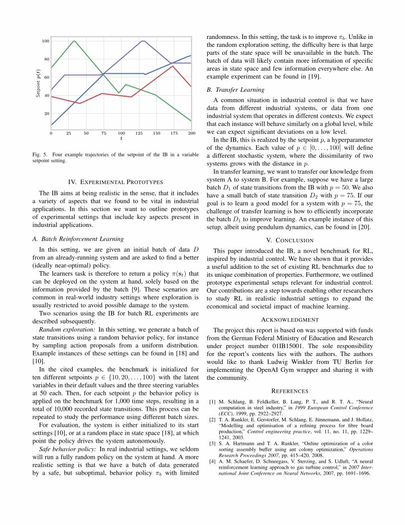
Setpoint p can either be kept constant or it is variable overtime. In the variable setting, it will change by a constantvalue b over a fixed period of l time steps in the benchmarkdynamics. Afterwards, a new sequence length and change rateis determined.

We sample sequence length l uniformly from U{1, 100} anddraw rate b from a mixture of a uniform distribution U(0, 1)and a delta distribution δ(x) with weighting probabilities 0.9and 0.1. For each time step t + 1 we update the setpointaccording to:

pt+1 = max(0,min(100, pt + bt+1)), (32)

bt+1 =

{−bt if (pt = 0 ∨ pt = 100) ∧ z < 0.5

bt else,(33)

where z ∼ U(0, 1) will flip change rate b with a probabilityof 50% if the setpoint reaches one of the two bounds atp = 0 or p = 100. Note that the equation above producespiecewise linear functions of constant change. We visualizedfour example trajectories in Figure 5.

0 25 50 75 100 125 150 175 200t

20

40

60

80

100S

etp

ointp(t

)

Fig. 5. Four example trajectories of the setpoint of the IB in a variablesetpoint setting.

IV. EXPERIMENTAL PROTOTYPES

The IB aims at being realistic in the sense, that it includesa variety of aspects that we found to be vital in industrialapplications. In this section we want to outline prototypesof experimental settings that include key aspects present inindustrial applications.

A. Batch Reinforcement Learning

In this setting, we are given an initial batch of data Dfrom an already-running system and are asked to find a better(ideally near-optimal) policy.

The learners task is therefore to return a policy π(st) thatcan be deployed on the system at hand, solely based on theinformation provided by the batch [9]. These scenarios arecommon in real-world industry settings where exploration isusually restricted to avoid possible damage to the system.

Two scenarios using the IB for batch RL experiments aredescribed subsequently.

Random exploration: In this setting, we generate a batch ofstate transitions using a random behavior policy, for instanceby sampling action proposals from a uniform distribution.Example instances of these settings can be found in [18] and[10].

In the cited examples, the benchmark is initialized forten different setpoints p ∈ {10, 20, . . . , 100} with the latentvariables in their default values and the three steering variablesat 50 each. Then, for each setpoint p the behavior policy isapplied on the benchmark for 1,000 time steps, resulting in atotal of 10,000 recorded state transitions. This process can berepeated to study the performance using different batch sizes.

For evaluation, the system is either initialized to its startsettings [10], or at a random place in state space [18], at whichpoint the policy drives the system autonomously.

Safe behavior policy: In real industrial settings, we seldomwill run a fully random policy on the system at hand. A morerealistic setting is that we have a batch of data generatedby a safe, but suboptimal, behavior policy πb with limited

randomness. In this setting, the task is to improve πb. Unlike inthe random exploration setting, the difficulty here is that largeparts of the state space will be unavailable in the batch. Thebatch of data will likely contain more information of specificareas in state space and few information everywhere else. Anexample experiment can be found in [19].

B. Transfer Learning

A common situation in industrial control is that we havedata from different industrial systems, or data from oneindustrial system that operates in different contexts. We expectthat each instance will behave similarly on a global level, whilewe can expect significant deviations on a low level.

In the IB, this is realized by the setpoint p, a hyperparameterof the dynamics. Each value of p ∈ [0, . . . , 100] will definea different stochastic system, where the dissimilarity of twosystems grows with the distance in p.

In transfer learning, we want to transfer our knowledge fromsystem A to system B. For example, suppose we have a largebatch D1 of state transitions from the IB with p = 50. We alsohave a small batch of state transition D2 with p = 75. If ourgoal is to learn a good model for a system with p = 75, thechallenge of transfer learning is how to efficiently incorporatethe batch D1 to improve learning. An example instance of thissetup, albeit using pendulum dynamics, can be found in [20].

V. CONCLUSION

This paper introduced the IB, a novel benchmark for RL,inspired by industrial control. We have shown that it providesa useful addition to the set of existing RL benchmarks due toits unique combination of properties. Furthermore, we outlinedprototype experimental setups relevant for industrial control.Our contributions are a step towards enabling other researchersto study RL in realistic industrial settings to expand theeconomical and societal impact of machine learning.

ACKNOWLEDGMENT

The project this report is based on was supported with fundsfrom the German Federal Ministry of Education and Researchunder project number 01IB15001. The sole responsibilityfor the report’s contents lies with the authors. The authorswould like to thank Ludwig Winkler from TU Berlin forimplementing the OpenAI Gym wrapper and sharing it withthe community.

REFERENCES

[1] M. Schlang, B. Feldkeller, B. Lang, P. T., and R. T. A., “Neuralcomputation in steel industry,” in 1999 European Control Conference(ECC), 1999, pp. 2922–2927.

[2] T. A. Runkler, E. Gerstorfer, M. Schlang, E. Junnemann, and J. Hollatz,“Modelling and optimisation of a refining process for fibre boardproduction,” Control engineering practice, vol. 11, no. 11, pp. 1229–1241, 2003.

[3] S. A. Hartmann and T. A. Runkler, “Online optimization of a colorsorting assembly buffer using ant colony optimization,” OperationsResearch Proceedings 2007, pp. 415–420, 2008.

[4] A. M. Schaefer, D. Schneegass, V. Sterzing, and S. Udluft, “A neuralreinforcement learning approach to gas turbine control,” in 2007 Inter-national Joint Conference on Neural Networks, 2007, pp. 1691–1696.

[5] A. Hans, D. Schneegass, A. M. Schaefer, and S. Udluft, “Safe explo-ration for reinforcement learning,” in 2008 European Symposium onArtificial Neural Networks (ESANN), 2008, pp. 143–148.

[6] M. G. Bellemare, Y. Naddaf, J. Veness, and M. Bowling, “The arcadelearning environment: An evaluation platform for general agents,” Jour-nal of Artificial Intelligence Research, vol. 47, pp. 253–279, 2013.

[7] E. Todorov, T. Erez, and Y. Tassa, “Mujoco: A physics engine formodel-based control,” in 2012 IEEE/RSJ International Conference onIntelligent Robots and Systems (IROS). IEEE, 2012, pp. 5026–5033.

[8] T. P. Lillicrap, J. J. Hunt, A. Pritzel, N. Heess, T. Erez, Y. Tassa,D. Silver, and D. Wierstra, “Continuous control with deep reinforcementlearning,” arXiv preprint arXiv:1509.02971, 2015.

[9] S. Lange, T. Gabel, and M. Riedmiller, “Batch reinforcement learning,”in Reinforcement Learning. Springer, 2012, pp. 45–73.

[10] D. Hein, S. Udluft, M. Tokic, A. Hentschel, T. A. Runkler, andV. Sterzing, “Batch reinforcement learning on the industrial benchmark:First experiences,” in 2017 International Joint Conference on NeuralNetworks (IJCNN), 2017, pp. 4214–4221.

[11] R. S. Sutton and A. G. Barto, Reinforcement Learning: An Introduction.Cambridge, MA: MIT Press, 1998.

[12] P. Abbeel, A. Coates, and A. Y. Ng, “Autonomous helicopter aerobaticsthrough apprenticeship learning,” The International Journal of RoboticsResearch, vol. 29, no. 13, pp. 1608–1639, 2010.

[13] J. Randløv and P. Alstrøm, “Learning to drive a bicycle using reinforce-ment learning and shaping,” in Proceedings of the Fifteenth InternationalConference on Machine Learning (ICML 1998), J. W. Shavlik, Ed. SanFrancisco, CA, USA: Morgan Kauffman, 1998, pp. 463–471.

[14] V. Mnih, K. Kavukcuoglu, D. Silver, A. A. Rusu, J. Veness, M. G.Bellemare, A. Graves, M. Riedmiller, A. K. Fidjeland, G. Ostrovski,S. Petersen, C. Beattie, A. Sadik, I. Antonoglou, H. King, D. Kumaran,D. Wierstra, S. Legg, and D. Hassabis, “Human-level control throughdeep reinforcement learning,” Nature, vol. 518, no. 7540, pp. 529–533,2015.

[15] H. van Seijen, M. Fatemi, J. Romoff, R. Laroche, T. Barnes, andJ. Tsang, “Hybrid reward architecture for reinforcement learning,” arXivpreprint arXiv:1706.04208, 2017.

[16] D. Silver, A. Huang, C. J. Maddison, A. Guez, L. Sifre, G. van denDriessche, J. Schrittwieser, I. Antonoglou, V. Panneershelvam, M. Lanc-tot, S. Dieleman, D. Grewe, J. Nham, N. Kalchbrenner, I. Sutskever,T. P. Lillicrap, M. Leach, K. Kavukcuoglu, T. Graepel, and D. Hassabis,“Mastering the game of Go with deep neural networks and tree search,”Nature, vol. 529, no. 7587, pp. 484–489, 2016.

[17] A. Hans and S. Udluft, “Efficient uncertainty propagation for rein-forcement learning with limited data,” in 2009 Proceedings of theInternational Conference on Artificial Neural Networks (ICANN 2009),2009, pp. 70–79.

[18] S. Depeweg, J. M. Hernandez-Lobato, F. Doshi-Velez, and S. Udluft,“Learning and policy search in stochastic dynamical systems withBayesian neural networks,” arXiv preprint arXiv:1605.07127, 2016.

[19] ——, “Uncertainty decomposition in Bayesian neural networks withlatent variables,” arXiv preprint arXiv:1706.08495, 2017.

[20] S. Spieckermann, S. Dull, S. Udluft, A. Hentschel, and T. A. Runkler,“Exploiting similarity in system identification tasks with recurrent neuralnetworks,” Neurocomputing, vol. 169, pp. 343–349, 2015.

APPENDIX ASTATE DESCRIPTION

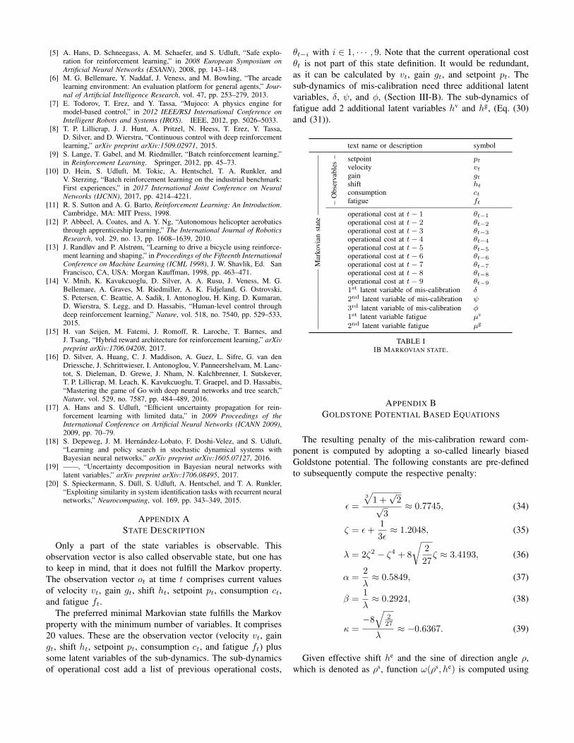
Only a part of the state variables is observable. Thisobservation vector is also called observable state, but one hasto keep in mind, that it does not fulfill the Markov property.The observation vector ot at time t comprises current valuesof velocity vt, gain gt, shift ht, setpoint pt, consumption ct,and fatigue ft.

The preferred minimal Markovian state fulfills the Markovproperty with the minimum number of variables. It comprises20 values. These are the observation vector (velocity vt, gaingt, shift ht, setpoint pt, consumption ct, and fatigue ft) plussome latent variables of the sub-dynamics. The sub-dynamicsof operational cost add a list of previous operational costs,

θt−i with i ∈ 1, · · · , 9. Note that the current operational costθt is not part of this state definition. It would be redundant,as it can be calculated by vt, gain gt, and setpoint pt. Thesub-dynamics of mis-calibration need three additional latentvariables, δ, ψ, and φ, (Section III-B). The sub-dynamics offatigue add 2 additional latent variables hv and hg, (Eq. (30)and (31)).

text name or description symbol

——

——

——

——

Mar

kovi

anst

ate

——

——

——

——

–O

bser

vabl

es– setpoint pt

velocity vtgain gtshift htconsumption ctfatigue ft

operational cost at t− 1 θt−1

operational cost at t− 2 θt−2

operational cost at t− 3 θt−3

operational cost at t− 4 θt−4

operational cost at t− 5 θt−5

operational cost at t− 6 θt−6

operational cost at t− 7 θt−7

operational cost at t− 8 θt−8

operational cost at t− 9 θt−9

1st latent variable of mis-calibration δ2nd latent variable of mis-calibration ψ3rd latent variable of mis-calibration φ1st latent variable fatigue µv

2nd latent variable fatigue µg

TABLE IIB MARKOVIAN STATE.

APPENDIX BGOLDSTONE POTENTIAL BASED EQUATIONS

The resulting penalty of the mis-calibration reward com-ponent is computed by adopting a so-called linearly biasedGoldstone potential. The following constants are pre-definedto subsequently compute the respective penalty:

ε =3√

1 +√

2√3

≈ 0.7745, (34)

ζ = ε+1

3ε≈ 1.2048, (35)

λ = 2ζ2 − ζ4 + 8

√2

27ζ ≈ 3.4193, (36)

α =2

λ≈ 0.5849, (37)

β =1

λ≈ 0.2924, (38)

κ =−8√

227

λ≈ −0.6367. (39)

Given effective shift he and the sine of direction angle ρ,which is denoted as ρs, function ω(ρs, he) is computed using

the following set of equations:

ω =

{(h

e|rmin|)|ropt| if |he| ≤ |ropt|

sgn(he) · ω else,(40)

ω = |rmin|+ 2− |rmin|(2− |ropt|) ˆω

· (|he| − |ropt|) ˆω, (41)

ˆω =2− |ropt|2− |rmin|

, (42)

ropt = % ·max(|ρs|, 2z), (43)

rmin =

{u+ 1

3u if q < −√

1/27

%√

43 cos

(13 · acos(−q

√27))

else,(44)

u =3

√−%q +

√q2 − 1

27, (45)

q =κ|ρs|8β

, (46)

% = sgn(ρs). (47)