arX

iv:1

410.

5820

v1 [

astr

o-ph

.SR

] 21

Oct

201

4DRAFT VERSIONOCTOBER23, 2014Preprint typeset using LATEX style emulateapj v. 5/2/11

HUBBLE SPACE TELESCOPE PROPER MOTION (HSTPROMO) CATALOGS OF GALACTIC GLOBULAR CLUSTERS∗.I. SAMPLE SELECTION, DATA REDUCTION AND NGC 7078 RESULTS

A. BELLINI 1, J. ANDERSON1, R. P.VAN DER MAREL1, L. L. WATKINS1, I. R. KING2, P. BIANCHINI 3, J. CHANAMÉ 4, R. CHANDAR5, A.M. COOL6, F. R. FERRARO7, H. FORD8, D. MASSARI7

Draft version October 23, 2014

AbstractWe present the first study of high-precision internal propermotions (PMs) in a large sample of globular

clusters, based onHubble Space Telescope(HST) data obtained over the past decade with the ACS/WFC,ACS/HRC, and WFC3/UVIS instruments. We determine PMs for over 1.3 million stars in the central regionsof 22 clusters, with a median number of∼60,000 stars per cluster. These PMs have the potential to significantlyadvance our understanding of the internal kinematics of globular clusters by extending past line-of-sight (LOS)velocity measurements to two- or three-dimensional velocities, lower stellar masses, and larger sample sizes.We describe the reduction pipeline that we developed to derive homogeneous PMs from the very heterogeneousarchival data. We demonstrate the quality of the measurements through extensive Monte-Carlo simulations. Wealso discuss the PM errors introduced by various systematiceffects, and the techniques that we have developedto correct or remove them to the extent possible. We provide in electronic form the catalog for NGC 7078(M 15), which consists of 77,837 stars in the central 2.′4. We validate the catalog by comparison with existingPM measurements and LOS velocities, and use it to study the dependence of the velocity dispersion on radius,stellar magnitude (or mass) along the main sequence, and direction in the plane of the sky (radial/tangential).Subsequent papers in this series will explore a range of applications in globular-cluster science, and will alsopresent the PM catalogs for the other sample clusters.Subject headings:Proper motions – Techniques: photometric – Stars: kinematics and dynamics, Population

II – (Galaxy): globular clusters: individual (NGC 104 (47 Tuc), NGC 288, NGC 362,NGC 1851, NGC 2808, NGC 5139 (ω Cen), NGC 5904 (M 5), NGC 5927, NGC 6266(M 62), NGC 6341 (M 92), NGC 6362, NGC 6388, NGC 6397, NGC 6441,NGC 6535,NGC 6624, NGC 6656 (M 22), NGC 6681 (M 70), NGC 6715 (M 54), NGC 6752,NGC 7078 (M 15), NGC 7099 (M 30))

1. INTRODUCTION

Globular clusters (GCs) are the oldest surviving stellar sys-tems in galaxies. As such, they provide valuable informationon the earliest phases of galactic evolution, and have been thetarget of numerous studies during the past century. Measuresof the stellar motions in GCs, for instance, allow us to con-strain the structure, formation, and dynamical evolution ofthese ancient stellar systems, and in turn, that of the MilkyWay itself.

Almost all of what is known about the internal motionswithin GCs is based on spectroscopic line-of-sight (LOS) ve-

bellini@stsci.edu∗ Based on proprietary and archival observations with the NASA/ESA

Hubble Space Telescope, obtained at the Space Telescope Science Insti-tute, which is operated by AURA, Inc., under NASA contract NAS 5-26555.

1 Space Telescope Science Institute, 3700 San Martin Drive, Baltimore,21218, MD, USA

2 Department of Astronomy, University of Washington, Box 351580,Seattle, WA 98195, USA

3 Max Planck Institute for Astronomy, Königstuhl 17, 69117 Heidel-berg, Germany

4 Istituto de Astrofísica, Pontificia Universidad Católica de Chile, Av.Vicuña Mackenna 4860, Macul 782-0436, Santiago, Chile

5 Department of Physics and Astronomy, The University of Toledo,2801 West Bancroft Street, Toledo, 43606, OH, USA

6 Department of Physics and Astronomy, San Francisco State Univer-sity, 1600 Holloway Avenue, San Francisco, CA 94132, USA

7 Dipartimento di Fisica e Astronomia, Università di Bologna, via Ran-zani 1, 40127 Bologna, Italy

8 Department of Physics and Astronomy, The Johns Hopkins University,3400 North Charles Street, Baltimore, 21218, MD, USA

locity measurements. Observations of the kinematics of GCshave come a long way since, e.g., Illingworth (1976) mea-sured the velocity dispersions of 10 clusters using the broad-ening of absorption lines in integrated-light spectra and DaCosta et al. (1977) measured the velocities for 11 stars inNGC 6397. The largest published samples today have ve-locities for a few thousand stars (e.g., Gebhardt et al. 2000;Malavolta et al. 2014, Massari et al. 2014).

Despite the major improvements provided by LOS-basedstudies on our understanding of the dynamics of GCs, thereare some intrinsic limitations. First of all, the need for spec-troscopy implies that only the brighter (more massive) starsin a GC can be observed. Moreover, in the crowded centralregions of the cluster core, spectroscopy is limited by sourceconfusion. Even integral-field spectroscopy is affected bytheshot noise from the brightest sources. Moreover, LOS mea-surements are limited to measure only one component of themotion, and therefore several model-dependent assumptionsare required to infer the three-dimensional structure of GCs.

A significant improvement in data quality is possible withproper-motion (PM) measurements. Indeed, PMs have the po-tential to provide several advantages over LOS velocity stud-ies: (1) No spectroscopy is required, so the more plentifulfainter stars can be studied, which yields better statistics onthe kinematical quantities of interest. (2) Stars are measuredindividually, in contrast with integrated-light measurements,which contain a disproportionate contribution from brightgi-ants. (3) Two components of velocity are measured insteadof just one. More importantly, it directly reveals the velocity-

2

dispersion anisotropy of the cluster, thus removing the mass-anisotropy degeneracy (Binney & Mamon 1982).

PMs are small, and difficult to measure with ground-basedtelescopes, where they require an enormous effort to achieveonly a modest accuracy, particularly for faint stars in crowdedfields (e.g., van Leeuwen et al. 2000; Bellini et al. 2009). Onthe other hand, the stable environment of space makes theHubble Space Telescope(HST) an excellent astrometric tool.Its diffraction-limited resolution allows it to distinguish andmeasure positions and fluxes for stars all the way to the cen-ter of most globular clusters. Apart from small changes dueto breathing, its point spread function and geometric distor-tion have been extremely stable over the two decades sincethe repair mission.

HST has the ability to measure PMs of unmatched qual-ity compared with any ground-based facility, and even in themost-crowded central regions of GCs. Our team has devel-oped methods to do this accurately (e.g., Anderson & King2003a; Bellini, Anderson & Bedin 2011). For instance, for aGC 5 kpc from the Sun, a dispersion of 10 kms−1 correspondsto∼ 0.42 masyr−1; with a WFC3/UVIS scale of 40 maspix−1

this gives∼ 0.1 pixel over a 10-year time baseline. Sinceour measurement techniques reach a precision of∼0.01 pixelper single exposure for bright, unsaturated sources, a tenthof a pixel is easy game, even for rather faint stars, so thatlarge numbers of proper motions depend only on the avail-ability of archival data. To date, detailedHST internal PMdynamics of GCs have been studied for only a handful of clus-ters: NGC 104 (47 Tuc, McLaughlin et al. 2006), NGC 7078(M 15, McNamara et al. 2003), NGC 6266 (McNamara et al.2011, 2012), and NGC 5139 (ω Cen, Anderson & van derMarel 2010) – but a deluge is now imminent; the project isdescribed by Piotto et al. (2014), and the first result paper hasbeen submitted (Milone et al. 2014).

With high-quality PM catalogs it will be possible to ad-dress, for a large number of GCs, many important topics: (1)Cluster-field separation, for a better identification of bona-fide cluster members for luminosity- and mass-function anal-yses and the study of binaries and exotic stars, and to provideclean samples of targets for spectroscopic follow-up. (2)In-ternal motions, to study in detail the kinematics and the dy-namics of GCs in general, and of each population componentin particular (with the aim of looking for fossil signaturesof distinct star-formation events). (3)Absolute motions, byestimating an absolute proper-motion zero point using back-ground galaxies as a reference frame (e.g., the series of papersstarting with Dinescu et al. 1997 and continuing as Casetti-Dinescu, and Bellini et al. 2010 using ground-based observa-tions, and Bedin et al. 2003, Milone et al. 2006, and Massariet al. 2013 usingHST). Absolute PMs, in conjunction withradial velocities, allow calculation of Galactic orbits ofGCs;At the same time the orbits that they exhibit are an indicatorof the shape of the Galactic potential. (4)Geometric distance,by comparing the LOS velocity dispersion with that on theplane of the sky (Rees 1995, 1997). This will provide a scaleof GC distances that is independent of those based on stel-lar evolution or RR Lyrae stars. (5)Cluster rotation on theplane of the sky, from the measure of the stellar velocities asa function of the position angle at different radial distances(e.g., Anderson & King 2003b).10 (6) Energy equipartition,from the analysis of stellar velocity dispersion as a function

10 Cluster rotations can also be measured spectroscopically,see, e.g., Pe-terson & Cudworth (1994); Bianchini et al. (2013).

of the stellar mass (e.g., Trenti & van der Marel 2013). (7)Mass segregation, by studying the stellar velocity dispersionas a function of the distance from the cluster center for differ-ent stellar masses. (8)(An)isotropy, by comparing tangentialand radial components of the stellar motion. (9)Full three-dimensional cluster dynamics, when also LOS velocities areknown. The availability of all the three components of themotion will directly constrain the three-dimensional velocityand phase-space distribution functions. (10)Constraints onthe presence of an intermediate-mass black hole, by lookingfor both fast-moving individual stars and for a sudden increasein the velocity-dispersion-profile near the center (e.g., van derMarel & Anderson 2010).

Unfortunately,HSThas executed only a very limited num-ber of programs specifically aimed at the study of internal PMdynamics of GCs. Even so, many GCs have been observedwith HST for dozens of different studies, and several of theseclusters have been observed on multiple occasions. Motivatedby the enormous scientific potential offered by high-precisionPM measurements of stars in GCs, we started a project toderive high-precision PM catalogs for all GCs with suitablemulti-epoch image material in theHSTarchive. This projectis part of – and uses techniques developed in the context of– the HST proper-motion (HSTPROMO) collaboration11, aset ofHSTprojects aimed at improving our dynamical under-standing of stars, clusters, and galaxies in the nearby Universethrough the measurement and interpretation of PMs (e.g., vander Marel et al. 2013).

The paper is organized as follows. In Section 2 we presentthe sample of GCs and data sets used for our study. In Sec-tions 3, 4 and 5 we describe our detailed procedures for rawdata reduction, astrometry, and PM measurements, respec-tively. In Section 6 we test the accuracy of our procedureson simulated data. Section 7 describes the effects of system-atic errors and how we mitigate their effects. In Section 8 wediscuss some of the kinematical quantities implied by the cat-alog of PMs for the GC NGC 7078 (M 15). Conclusions arepresented in Section 9. Appendices present tables (availableelectronically) with listings of theHSTdata sets we used foreach cluster, and with the NGC 7078 PM catalog.

This is the first of a series of several papers. Future papersin this series will present the PM catalogs for the other GCs inour sample, will discuss the kinematical quantities they implyfor these GCs, and will address many of the scientific topicslisted above.

2. SAMPLE SELECTION

This work is based on archivalHST images taken withthree different cameras: (1) the Ultraviolet-Visible channel ofthe Wide-Field Camera 3 (WFC3/UVIS); (2) the Wide-FieldChannel of the Advanced Camera for Surveys (ACS/WFC);and (3) the High-Resolution Channel of ACS (ACS/HRC).

The physical characteristics of these cameras are as fol-lows: the WFC3/UVIS camera is made up of two 4096×2048-pixel chips, with a pixel-scale of about 40 maspixel−1;ACS/WFC has the same number of resolution elements as theWFC3/UVIS , but it has a larger sampling of 50 maspixel−1;ACS/HRC is theHST instrument with the finest resolution,being about 25 maspixel−1, and it is made up of a single chipof 1024 pixels on each side.

Wide-Field Planetary Camera 2 (WFPC2) exposures were

11 For details see the HSTPROMO home page athttp://www.stsci.edu/~marel/hstpromo.html.

3

TABLE 1GLOBULAR CLUSTERS AND THEIRPARAMETERS

Cluster ID R.A.⊲ Dec.⊲ D⊙∗ [Fe/H]∗ E(B−V)∗ σVLOS

∗ rc∗ rh

∗

(h:m:s) (◦:′:′′) kpc kms−1 ′ ′

NGC 104 (47 Tuc) 00:24:05.71 −72:04:52.7 4.5 −0.72 0.04 11.0±0.3 0.36 3.17NGC 288 00:52:45.24 −26:34:57.4 8.9 −1.32 0.03 2.9±0.3 1.35 2.23NGC 362 01:03:14.26 −70:50:55.6 8.6 −1.26 0.05 6.4±0.3 0.18 0.82NGC 1851 05:14:06.76 −40:02:47.6 12.1 −1.18 0.02 10.4±0.5 0.09 0.51NGC 2808 09:12:03.10 −64:51:48.6 9.6 −1.14 0.22 13.4±1.2 0.25 0.80

NGC 5139 (ω Cen) 13:26:47.24⋄ −47:28:46.45⋄ 5.2 −1.53 0.12 16.8±0.3 2.37 5.00NGC 5904 (M 5) 15:18:33.22 +02:04:51.7 7.5 −1.29 0.03 5.5±0.4 0.44 1.77

NGC 5927 15:28:00.69 −50:40:22.9 7.7 −0.49 0.45 8.8† 0.42 1.10NGC 6266 (M 62) 17:01:12.78‡ −30:06:46.0‡ 6.8 −1.18 0.47 14.3±0.4 0.22 0.92NGC 6341 (M 92) 17:17:07.39 +43:08:09.4 8.3 −2.31 0.02 6.0±0.4 0.26 1.02

NGC 6362 17:31:54.99 −67:02:54.0 7.6 −0.99 0.09 2.8±0.4 1.13 2.05NGC 6388 17:36:17.23 −44:44:07.8 9.9 −0.55 0.37 18.9±0.8 0.12 0.52NGC 6397 17:40:42.09 −53:40:27.6 2.3 −2.02 0.18 4.5±0.2 0.05 2.90NGC 6441 17:50:13.06 −37:03:05.2 11.6 −0.46 0.47 18.0±0.2 0.13 0.57NGC 6535 18:03:50.51 −00:17:51.5 6.8 −1.79 0.34 2.4±0.5 0.36 0.85NGC 6624 18:23:40.51 −30:21:39.7 7.9 −0.44 0.28 5.4±0.5 0.06 0.82

NGC 6656 (M 22) 18:36:23.94 −23:54:17.1 3.2 −1.70 0.34 7.8±0.3 1.33 3.36NGC 6681 (M 70) 18:43:12.76 −32:17:31.6 9.0 −1.62 0.07 5.2±0.5 0.03 0.71NGC 6715 (M 54) 18:55:03.33 −30:28:47.5 26.5 −1.49 0.15 10.5±0.3 0.09 0.82

NGC 6752 19:10:52.11 −59:59:04.4 4.0 −1.54 0.04 4.9±0.4 0.17 1.91NGC 7078 (M 15) 21:29:58.33 +12:10:01.2 10.4 −2.37 0.10 13.5±0.9 0.14 1.00NGC 7099 (M 30) 21:40:22.12 −23:10:47.5 8.1 −2.27 0.03 5.5±0.4 0.06 1.03

⊲ From Goldsbury et al. (2010), unless stated otherwise.∗ From Harris 1996 (2010 edition), unless stated otherwise.D⊙ is the GC distance from the Sun.⋄ From Anderson & van der Marel (2010).† From Gnedin et al. (2002).‡ From Beccari et al. (2006).

not taken into account because, despite the larger time base-line they can generally provide, there would be only amarginal increase in PM accuracy, due primarily to the largerpixel size (larger position uncertainties) and the smallerdy-namical range of the WFPC2 chips (fewer well-measuredstars), particularly in the crowded cores, which is the focusof this study.

Ten GCs were specifically observed withHST by some ofus to study their internal motions, namely:

• NGC 362, NGC 6624, NGC 6681, NGC 7078,NGC 7099 (GO-10401, PI: R. Chandar);

• NGC 2808, NGC 6341, NGC 6752 (GO-10335 andGO-11801, PI: H. Ford);

• NGC 6266, (GO-11609, PI: J. Chanamé);

• NGC 6715 (GO-12274, PI: R. P. van der Marel).

In January 2011 we searched through theHSTarchive to lookfor other suitable data and additional GCs, imaged with thethree aforementioned cameras and with a total time baselineof at least 2 years. Twelve GCs were found satisfying thesetwo criteria, and we successfully submitted an archivalHSTproposal (AR-12845, PI: A. Bellini) to analyze them. Theclusters are: NGC 104, NGC 288, NGC 1851, NGC 5139,NGC 5904, NGC 5927, NGC 6362, NGC 6388, NGC 6397,NGC 6441, NGC 6535 and NGC 6656. A summary of thegeneral properties for all 22 GCs is given in Table 1. A com-plete list of observations used for our analysis of each clustercan be found in the appendix.

3. DATA REDUCTION

3.1. Measuring Stellar Position and Fluxes in each Exposure

This work is based solely on_flt or _flc type images.These images are produced by the standardHST calibrationpipeline CALWF3 (for WFC3) or CALACS(for ACS). Im-ages of type_flt are dark- and bias-subtracted and flat-fielded, but not resampled (like the_drz type images);_flcimages are_flt exposures that are also charge-transfer-efficiency (CTE) corrected (see below). The choice to usenon-resampled images is motivated by the fact that we needto retain information about where exactly a photon hit the de-tector in order to minimize systematic errors in the PMs.

3.1.1. Charge-Transfer Efficiency Corrections

Charge-transfer errors arise from the damaging effects ofcosmic rays on the detectors. CTE losses affect both the shape(and therefore, position) and the measured flux of stars, andthese errors increase over time (see, e.g., Anderson & Bedin2010). CTE effects are more severe when the image back-ground is low, e.g. for short-exposures or when bluer filtersare used. It is a crucial step to properly model and correctthese CTE losses if we want to measure high-quality PMs.

The CTE correction for ACS is especially important onexposures taken after the camera was repaired in 2009 (7years after its installation), while CTE damage is only mildormarginal on earlier exposures. For the WFC of ACS, the CTEcorrection is already included in theCALACSpipeline (_flcextension). The correction is not available for the HRC ofACS, but this is only a minor issue, as the HRC stopped op-erating in 2006 and it was not repaired during the lastHSTService Mission 4 (SM4). Moreover, the HRC read-out alsohas a maximum of 1024 transfers, so that at its worst its CTElosses are only half as bad as the WFC.

An official CTE correction for WFC3/UVIS has been re-

4

cently made available, but it had not been implemented withinthe WFC3 calibration pipeline at the time of our reduc-tions. So we manually corrected each individual WFC3/UVIS_flt exposure with the stand-alone CTE correction routineavailable on the official UVIS website12 to create_flc im-ages.

3.1.2. ACS/WFC

All ACS/WFC _flc images were reduced us-ing the publicly-available FORTRAN programimg2xym_WFC.09x10, which is described in detailin Anderson & King (2006a).13 The program does a singlepass of finding and measures each star in each exposure byfitting a spatially-varying effective point spread function(PSF), ignoring any contribution from neighbors.

Library PSFs for several filters are provided along withthe reduction software. To take into account the variation ofthe PSF across the Field-of-View (FoV), the library PSFs aremade up of an array of 9×10 PSFs across the detector. At anygiven location on the detector, the local PSF is then obtainedthrough a bi-linear interpolation of the four surrounding li-brary PSFs.

During its∼ 90 min. orbital period around the Earth,HSTis cyclically heated by the Earth and Sun. As a result, the focallength changes slightly during each orbit. This effect, knownas “telescope breathing”, affects the shape of the PSF in anon-constant way across the field of view (FoV). To take intoaccount the time-dependent variations of the PSFs, for eachindividual exposure we derived an additional array of up to5×5 perturbation PSFs by modeling the residuals of library-PSF-subtracted stars across the detector. These perturbationPSFs were then interpolated into the 9×10 array of the libraryPSFs and added to them. The final set of PSFs (one set foreach exposure) was then used to fit stellar profiles.

3.1.3. WFC3/UVIS

Star positions and fluxes on WFC3/UVIS images were mea-sured with the softwareimg2xym_wfc3uv, adapted mostlyfrom img2xym_WFC.09x10. Library, spatially-varyingPSFs are available also for this detector (in an array of 7×8PSFs). As done for the ACS/WFC, we derived an additionalarray of perturbation PSFs for each WFC3/UVIS exposureand combined it with the library PSFs to fit stellar profiles.(For a more comprehensive analysis of spatial and time vari-ations of UVIS PSFs see Sabbi & Bellini 2013).

3.1.4. ACS/HRC

The measurement of stellar fluxes and positions in eachACS/HRC image was performed by using the publicly avail-able routineimg2xym_HRC and library PSFs. Because ofthe small FoV of HRC, there was no need to create spatially-varying PSFs, and a constant PSF for each filter is adeguate toproperly represent stellar profiles all across the detector. Weinvestigated the possibility of taking into account the time-dependent part of the PSFs but found that perturbation PSFswere able to provide only a negligible improvement in mod-eling stellar profiles.

3.2. Single-Exposure Catalogs

12 http://www.stsci.edu/hst/wfc3/tools/cte_tools.13 http://www.stsci.edu/~jayander/ACSWFC_PSFs/.

Theimg2xym-routine family used here produces a catalogof positions and fluxes of each measured star in each individ-ual exposure, together with some other additional quantitiesand diagnostics, such as the quality-of-fit (QFIT) parameter,which tells us how well a source has been fit with the PSFmodel (Anderson et al. 2008).

Neighbor subtraction was not taken into account, so starswere measured as they are on the exposures. Our aim is tomeasure PMs as precisely as possible, so we decided to focusour attention on relatively isolated stars, for which positionscan be reliably measured on individual exposures. The posi-tions of blended stars, or stars for which the profile is impairedby brighter neighbors, would be affected by systematics inany case (see Section 7.5).

The precision with which we are able to measure positionsfor well-exposed stars on a single image is of the order of. 0.01 pixels (See Section 5.2). This level of precision can beachieved thanks to the high quality of the carefully-modeled,fully-empirical PSFs at our disposal.

3.3. Geometric-Distortion Corrections

Stellar positions in each individual exposure were cor-rected for geometric distortion using the state-of-the-art so-lutions available for ACS/WFC (Anderson & King 2006a),ACS/HRC (Anderson & King 2006b), and WFC3/UVIS(Bellini & Bedin 2009; Bellini, Anderson & Bedin 2011).These corrections are able to provide distortion-free stellarpositions with residuals of the order of. 0.01 pixel (aboutthe same precision offered by the PSF-fitting). This level ofprecision in the distortion solution depends strongly on theadopted PSFs, and cannot be achieved with simple centroid-type approaches, with opticts-based PSFs, or even with empir-ical PSFs that do not adeguately treat the PSF’s spatial varia-tions.

WFC3/UVIS is affected by a chromatic dependence of thegeometric distortion, and the effect is larger for the bluerfil-ters (see, e.g., Fig. 6 of Bellini, Anderson & Bedin 2011).The problem likely resides in the fused-silica CCD windowswithin the optical system, which refract blue and red photonsdifferently and exhibit a sharp increase of the refractive indexin the ultraviolet regime.

We showed in Bellini, Anderson & Bedin( 2011) that thereare negligible color-dependent residuals in the UVIS distor-tion solutions for filters redward of F275W. A similar chro-matic dependence of the distortion solution might also bepresent for the bluer filters of ACS/HRC. To minimize thissubtle systematic effect, we decided to exclude any exposuretaken through filters bluer than F336W for UVIS, and F330Wfor HRC.

The bluest filter available for ACS/WFC peaks at 435 nm(F435W), and no chromatic dependence of the distortion solu-tion has been reported for this camera. The ACS/WFC, how-ever, experienced a slight change in the geometric-distortionsolution after it was repaired during SM4. Post-SM4 posi-tional residuals obtained with pre-SM4 geometric-distortionsolutions can be of the order of 0.05 pixels, and therefore needto be corrected. We carefully modeled the post-SM4 deviationof the distortion solution with a look-up table of residuals.14

The accuracy of the post-SM4 geometric-distortion solutionsfor the ACS/WFC are comparable with the pre-SM4 solution,and is of the order of. 0.01 pixels.

14http://www.stsci.edu/~jayander/ACSWFC_PSFs/POST-SM4/.

5

4. THE MASTER FRAME

The 22 GCs for which we want to measure PMs all have dif-ferent apparent size and core density. Moreover, most of thearchival data come from projects with scientific goals otherthan high-precision astrometry. As a result, the data sets at ourdisposal are extremely heterogeneous in terms of used cam-eras, filters, chosen exposure time, dither strategy, number ofexposures and time baseline.

Despite the severe lack of similarity among the data sets, itis important to be able to measure PMs for all 22 clusters ina homogeneous and standardized fashion. This eases subse-quent analyses and comparisons of the dynamical propertiesof each cluster. To obtain a homogeneous set of PM catalogswe had to address several issues.

The first issue concerns the definition of the reference sys-tem (master frame) on which to register the stellar positions.The master frame needs to be defined in a consistent way foreach cluster, and to have the same properties. Luckily, there isone data set in common between all but one GC (NGC 6266):GO-10775, PI: A. Sarajedini. This data set has been reducedwith software tools similar to the ones we employed here (formore details see Anderson et al. 2008). Its astro-photometriccatalogs are publicly available15, and their high quality andreliability are supported by several dozens of papers. More-over, the GO-10775 data were taken in 2006, and usually liein between the time baseline of the data sets of each cluster,thus limiting bias effects in computing PMs.

The GO-10775 catalogs have stellar positions in equato-rial units and in ACS/WFC pixels (rescaled to be exactly 50maspixel−1). The pixel-based reference frame has North upand East to the left, and places the center of each GC (asdefined in Harris 1996) at location (3000, 3000). To betterexploit the GO-10775 catalogs as our reference systems, weapplied the following three changes:

1. We modified the pixel scale from 50 to 40 maspixel−1,which is the WFC3/UVIS pixel scale, and represents acompromise between the ACS/HRC and the ACS/WFCpixel scales).

2. We shifted the cluster-center positions to location(5000, 5000), in order to accommodate all overlappingdata sets with GO-10775 (which have different point-ings and orientations) without having to deal with neg-ative coordinates.

3. We removed from the GO-10775 catalogs those starsfor which the position was not well measured, follow-ing the prescriptions given in Anderson et al. (2008).In addition, we removed stars belonging to any of thefollowing cases: (1) saturated stars; (2) stars fainterthan instrumental magnitude16 −5.7 in either F606Wor F814W; (3) stars with positional error larger than 5

15http://www.astro.ufl.edu/~ata/public_hstgc/data-bases.html.

16 The instrumental magnitude is defined as−2.5× log(flux), where theflux in counts is the volume under the PSF that best fits a stellar profile.Wewill use instrumental magnitudes extensively throughout this paper, as theyoffer an immediate sense of the signal-to-noise ratio of measured sources.As a reference, a typicalHST central PSF value is∼ 0.2 (i.e., 20% of thesource flux is in its central pixel): this means that saturated stars (central pixel≥ 55000 counts) will have magnitudes brighter than instrumental magnitude−2.5× log(55000/0.2) =−13.6. Moreover, stars with instrumental magnitude−10 will have a signal-to-noise ratio of 100.

mas in either coordinate; (4) stars with photometric er-ror larger than 0.2 mag in either filter; and (5) stars withoV or oI , i.e. the ratio of neighbor vs. star light in theaperture greater than 1.

Although a GO-10775 catalog is available forω Cen, wedecided instead to base its reference system on the GO-9442data set (PI: A. Cool). The reason for this is twofold: (1)the GO-9442 field of view is nine times larger than that ofGO-10775, and there are other projects (such as GO-10252)that overlap with GO-9442 but not with GO-10775, thus al-lowing PM measurements at larger radial distances; and (2)the GO-9442 observation strategy was very similar to that ofGO-10775 in terms of dithering scheme, number of exposuresand exposure time. Only the chosen filters are different, onaccount of the different scientific goals. Moreover, data ofGO-9442 were reduced by one of us (J. Anderson) with apreliminary version of the same software used to create theGO-10775 database. To transform the GO-9442 catalog intoour reference system, we applied the same aforementionedchanges applied to GO-10775 catalogs.

In order to obtain a reference system for NGC 6266, wenoted that the data of GO-10210 were taken following a verysimilar observing strategy to that of GO-9442 forω Cen.Therefore we reduced GO-10120 following the prescriptionsgiven in Anderson et al. (2008) to produce a star catalog anal-ogous to those of GO-10775, and we applied the same threechanges as for the GO-10775 data sets.

5. PROPER MOTIONS

In the simple situation of repeated observations taken inonly two epochs, one can simply measure the average posi-tion of stars within each epoch, and then obtain PMs as thedifference in position between the second and the first epoch,divided by the time baseline. In reality, our data sets gen-erally contain a varying number of epochs, sometimes withone exposure only. Even when there are multiple exposureswithin a given epoch (which may span several weeks), starsare usually measured through different filters and with differ-ent exposure times –and hence different signal-to-noise–,andit is not trivial to properly determine an average position forthem within each epoch. Therefore, we decided to treat eachindividual exposure as a stand-alone epoch, and to measurePMs by fitting a straight line to the data in the position versusepoch space (essentially the so-calledcentral overlapmethod,first proposed by Eichhorn & Jefferys 1971).

Our general strategy for measuring PMs can be summarizedinto five main steps: (1) measure stellar positions in each in-dividual exposure; (2) cross-identify the same stars in alltheexposures where they can be found; (3) define a reference net-work of stars with respect to which we can compute PMs; (4)transform stellar positions onto a common reference frame;(5) fit straight lines to the reference-frame-position-versus-epoch data to obtain PMs.

Steps (3), (4) and (5) are nested into each other, and eachof them requires some iteration in order to reject discrepantobservations and improve the PM measurements. The basicscheme of the iterative process is summarized in the flow-chart of Fig. 1. We have already discussed step (1) in Section3; the following subsections will provide a comprehensive ex-planation of the subsequent steps.

5.1. Linking master-frame to single-catalog stellar positions

6

Figure 1. Flow chart illustrating the adopted scheme to compute PMs. The three main steps discussed in the text are marked as (S3), (S4) and (S5). See Sections5.3, 5.4 and 5.5, respectively, for details.

First of all, each star in the master-frame list needs to beidentified in each individual exposure where it can be found.The cross-identification is performed by means of general six-parameter linear transformations. These allow us to transformstellar positions as measured in the individual exposures ontothe reference system, and associate them with the closest starof the master frame list.

We are matching up stars that have moved in random di-rections as time has passed. To limit the number of mis-matches, we considered only stars from which master-framematches are within 2.5 pixels (0.′′1). This criterion neces-sarily limits our ability to measure the motion of very-fast-moving stars. As an example, let us take the NGC 5927data set. The time baselines to the reference dataset (GO-10775) is 3.87 years for GO-9453 and about 4.38 years forGO-11664 and GO-11729. The fastest motion we can mea-sure for stars present only in the GO-10775 and GO-9453 datais µ = 2.5×40/3.87 mas yr−1 = 25.84 mas yr−1. This limit isfurther reduced to 22.83 masyr−1 if stars are measured in theGO-11664 and/or GO-11729 data sets but not in the GO-9453one (see also Table A8). These PMs correspond to∼ 940kms−1 and 830 kms−1 at the distance of NGC 5927, but wouldcorrespond to smaller velocities for foreground stars.

At the initial stage, there is no need to fine-tune the lin-ear transformations, so long as we are able to identify master-frame stars in each exposure. We will later compute improvedtransformations to precisely place single-exposure stellar po-sitions onto the master frame.

5.2. Expected errors

Since each exposure corresponds to a stand-alone epoch,we cannot directly measure stellar positional errors from theRMS of the residuals around an epoch-averaged position, asin the case of multiple exposures per epoch. Instead, we needto assign an a-priori expected error based on some assump-tions.

We reduced thousands ofHST images and found as ex-pected that there is a general trend of increasing positionalRMS as a function of the instrumental magnitude. This trendis stable over time and has little dependence on the filter used.For this reason, we decided to model this trend for the three

Figure 2. Modeling of the expected errors for the ACS/WFC camera. Thetop three panels show the 1D positional RMS as a function of the instrumen-tal magnitude for three filters of the central field ofω Cen. We computedthe 68.27 percentile of these RMS in bins of 0.2 mag, and fitteda 5th-orderpolynomial to them. The bottom two panels show the binned RMSin linearand logarithmic units, together with the fitted function.

HST detectors employed here and assign an expected posi-tional error to each star of each individual catalog accordingto its instrumental magnitude.

To model the ACS/WFC expected-error trend, we chose theexposures of the core ofω Cen, a moderately-crowded fieldcontaining several thousand stars, and imaged through sev-eral dithered exposures in the F435W, F606W and F814W fil-ters (to sample the available wavelength coverage). For eachfilter, we computed average star magnitudes and positions,and measured the positional RMS of the residuals about themean. Stars brighter than instrumental magnitude∼ −13.7are saturated and were not taken into account. Stars fainterthan∼ −5.7 are generally close to the shot-noise level for

7

single-exposure measurements, and define the faint limit ofthe model.

The top three panels of Fig. 2 show one-dimensional posi-tional RMS as a function of the instrumental magnitude forF814W, F606W and F435W from top to bottom. We dividedeach sample of points in bins of 0.2 mag, and computed a 3σ-clipped 68.27 percentile of the positional RMS within eachbin (full colored circles). The bottom two panels of the figureshow sampled values of the three filters, in linear and logarith-mic units, as a function of the instrumental magnitude. Thelogarithmic units allow one to better distinguish the sampledvalues in the bright regime, while the linear units work betterfor the faint regime. A least-squares 5th-order polynomialisfit to the points in the log plane to model the positional RMStrend. This model provides our expected errors for the ACS/WFC camera.

For the ACS/HRC and the WFC3/UVIS cameras we usedthe central fields of 47 Tuc andω Cen, respectively17, andfollowed the same procedures used for the ACS/WFC camerato model the positional RMS, and thus the expected errors,as a function of the instrumental magnitude. For these twodetectors we again modeled the expected errors using threefilters: a blue, an intermediate and a red filter. As for theACS/WFC, the intermediate and red filters are the F606Wand the F814W. As the blue filter for ACS/HRC we choseF475W instead of the ACS/WFC F435W, because F475W ex-posures are more numerous and have longer exposure times.Because the WFC3/UVIS detector covers bluer wavelengthsthan the ACS/WFC, the adopted blue filter was the F336W(which is also the bluest filter used to compute PMs). The av-erage modeled curves of the expected errors for the ACS/HRCand the WFC3/UVIS cameras are very similar to those for theACS/WFC shown in Fig. 2.

5.3. The Reference-Star List

At this stage in the reduction process, we are ready to startmeasuring PMs. We want to stress here that we will com-puterelative and notabsolutePMs. The main reason is thatthe cores of GCs are so dense that the light of a backgroundgalaxy can hardly push itself above the scattered light of thecluster. (One of the few clusters in which there are enoughgalaxies to actually measure absolute PMs is NGC 6681,see Massari et al. 2013.) Therefore, in general we need tochoose a reference set of objects other than background galax-ies against which to measure motions. This leaves the clusterstars and the field stars. The cluster stars have a much tighterPM distribution, so they are the obvious choice. Our motionswill thus be in a frame that moves and rotates with the cluster.

We want to use only the best-measured, unsaturated master-frame stars in order to minimize transformation residuals.Master-frame magnitudes are rezo-pointed with respect to thedeep exposures of GO-10775, therefore the short-exposuresaturation limit in instrumental magnitudes is about−16.5,and the long-exposure limit is about−13.5. Stars between−16.5 and−13.5 mag are measured only in the short expo-sures. Generally, the best-measured stars lie within∼ 3 magof the saturation limit. Therefore, in principle we could con-sider all stars between instrumental magnitude−16.5 and−10in our reference list. However, because of the large varietyofexposure times in our data sets, it could be that these brightstars are too bright (i.e., saturated) in some exposures. We

17 No suitable ACS/HRC exposures of the core ofω Cen have been taken,while the core of 47 Tuc was used as ACS/HRC calibration field.

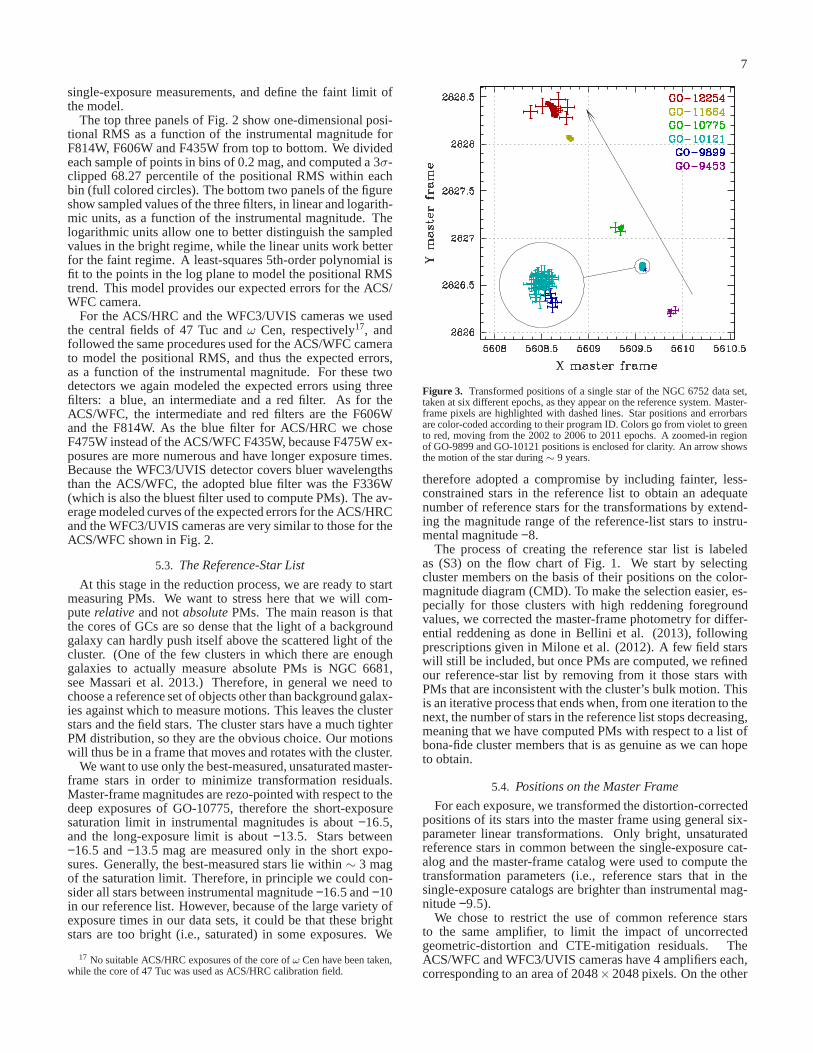
Figure 3. Transformed positions of a single star of the NGC 6752 data set,taken at six different epochs, as they appear on the reference system. Master-frame pixels are highlighted with dashed lines. Star positions and errorbarsare color-coded according to their program ID. Colors go from violet to greento red, moving from the 2002 to 2006 to 2011 epochs. A zoomed-in regionof GO-9899 and GO-10121 positions is enclosed for clarity. An arrow showsthe motion of the star during∼ 9 years.

therefore adopted a compromise by including fainter, less-constrained stars in the reference list to obtain an adequatenumber of reference stars for the transformations by extend-ing the magnitude range of the reference-list stars to instru-mental magnitude−8.

The process of creating the reference star list is labeledas (S3) on the flow chart of Fig. 1. We start by selectingcluster members on the basis of their positions on the color-magnitude diagram (CMD). To make the selection easier, es-pecially for those clusters with high reddening foregroundvalues, we corrected the master-frame photometry for differ-ential reddening as done in Bellini et al. (2013), followingprescriptions given in Milone et al. (2012). A few field starswill still be included, but once PMs are computed, we refinedour reference-star list by removing from it those stars withPMs that are inconsistent with the cluster’s bulk motion. Thisis an iterative process that ends when, from one iteration tothenext, the number of stars in the reference list stops decreasing,meaning that we have computed PMs with respect to a list ofbona-fide cluster members that is as genuine as we can hopeto obtain.

5.4. Positions on the Master Frame

For each exposure, we transformed the distortion-correctedpositions of its stars into the master frame using general six-parameter linear transformations. Only bright, unsaturatedreference stars in common between the single-exposure cat-alog and the master-frame catalog were used to compute thetransformation parameters (i.e., reference stars that in thesingle-exposure catalogs are brighter than instrumental mag-nitude−9.5).

We chose to restrict the use of common reference starsto the same amplifier, to limit the impact of uncorrectedgeometric-distortion and CTE-mitigation residuals. TheACS/WFC and WFC3/UVIS cameras have 4 amplifiers each,corresponding to an area of 2048×2048 pixels. On the other

8

hand, the ACS/HRC camera has only one amplifier, thereforethis restriction does not apply.

The geometric distortion has a smooth variation across thedetectors, and therefore it can be considered locally flat. If wewere to use the local-transformation approach (see, e.g., An-derson et al. 2009; Bellini et al. 2009), we would have min-imized the impact of uncorrected geometric-distortion resid-uals. However, the adopted amplifier-type restriction (a sortof semi-local approach) allows us to limit these effects. Wewill henceforth refer to the PMs thus obtained as "amplifier-based". This in contrast to "locally-corrected" PMs, whichare discussed in Section 7.3. Both types of PMs are listedin our catalogs. Which PMs are best depends on the specificscientific application.

Concerning CTE-correction residuals, y-CTE effects (i.e.,trails along the Y axis of the detector), vary as a function oftheir distance from the register. Each amplifier has its ownregister. To date, there is no pixel-based x-CTE correction(i.e.,trails along the X axis) available forHST. However, theimpact of x-CTE effects is order of magnitudes smaller thanthat of y-CTE, and to the first order, it should be compensatedfor by our amplifier-based approach.

Since all the stars in our reference list are moving in ran-dom directions with respect to each other with some disper-sion, each and every transformed star position is affected bya systematic error of err∝

√

σref/Nref, whereNref is the to-tal number of reference stars used for the transformation andσref their PM dispersion. This implies that a large number ofreference stars is best to minimize this source of error. Onthe other hand, it is not uncommon to have only a handfulof reference stars to use for the transformations, especiallyin partially-overlapping data sets, or when the image depthis very different. A good compromise for the used data setswas found by rejecting all transformed stars that had less than75 reference stars within their amplifier for ACS/WFC andWFC3/UVIS exposures, and less than 50 for ACS/HRC ex-posures. In the vast majority of cases, the typical number ofreference stars used for the transformations is larger than300.

As mentioned, the reference stars do also move themselves.As a result, when we transform stellar positions of exposurestaken years apart from the master-frame epoch, we will neces-sarily have to deal with larger transformation residuals. Theseresiduals will in turn translate into larger uncertaintiesin thetransformed positions of stars. We can bypass this problem bycorrecting the positions of the reference stars to correspond tothe epoch of the single-exposure catalog that we want to trans-form.

Obviously, we need to know the PM of the reference stars tocompute their position adjustments. As a consequence, com-puting positions on the master frame is an iterative process.With improved transformations we will be able to measuremore precise PMs, and with them obtain even better transfor-mations. We found that 5 iterations were enough to minimizethe transformation residuals.

Once all the stars of all the exposures are transformed intothe master frame, each master-frame star will be characterizedby several slightly different positions, each of them referringto a different exposure (i.e., a different epoch). In Fig. 3 weillustrate this concept for a rapidly-moving star in the fieldof NGC 6752. On the master frame (the pixels of which arehighlighted by dashed lines), each point represents a trans-formed single-exposure position. Errorbars are obtained us-ing expected errors (from Sectio. 5.2), sp that larger errorbars

refer to shorter exposure times. For clarity, we color-codedstar positions according to their program number. The epochsof the observations go from 2002 (GO-9453, purple data) to2011 (GO-12254, red data). We recall that the master-frameepoch is defined by the GO-10775 observations (in green).The actual master-frame position of this star lies underneaththe green points (not shown). Data of GO-9899 and GO-10121 are separated by less than 3 months, and their positionis magnified in the enclosed circle. An arrow indicates themotion of the star over∼ 9 years.

5.5. Proper-Motion Fitting and Data Rejection

Let us suppose that for a given star we haveN total positionsin the master frame. Each position has an associated expectedone-dimensional error and an epoch of observation, and istherefore characterized by the quadruplet (xN,yN,eN, tN). Tomeasure the motion of this star along the X and Y axes, weused a weighted least-squares to fit a straight line to the datapoints (xN, tN) and (yN, tN). We progressively improve the fitby rejecting outliers or badly-measured observations. This it-erative straight-line-fitting process is marked as (S5) in theflow chart of Fig. 1.

We require that a star have at least 4 data points, with atleast 6 months of time baseline between the second and thesecond-from-last point, in order for its PM to be measured.These conditions must be satisfied at every stage of the fit-ting/rejection process.

Before starting with the iterative process, we identify andreject obvious outliers. This task is done by removing onepoint at a time, then fitting the straight lines to the remainingN − 1 points. If the distance of a removed point from its as-sociated fitted line is larger than 10 times its expected error,the point is rejected immediately. Such data points generallycome from objects with a cosmic-ray event within their fittingradius. As a result, the centroid is shifted toward the cosmicray, and their measured luminosity is enhanced by the cosmic-ray counts.

Let us suppose that a star still hasN data points after thesepreliminary selections. We fit two weighted straight lines tothe points (xN, tN) and (yN, tN). An example of these fits for thesame star used in Fig. 3 is illustrated in Fig. 4. Data points arecolor-coded as in Fig. 3. Panel (a) of Fig. 4 shows the fittedline in the X-position versus epoch plane, where the epochof each point is expressed relative to the master-frame epoch(T=0, in years). Panel (c) shows the fit for the Y-positionversus epoch. Panels (b) and (d) show the residuals (dxN,dyN)of the points around the straight-line fits.

To identify and reject the marginal outliers we adoptedthe one-point-at-a-time approach as follows: We define error-normalized quantitiesdx′N = dxN/eN, dy′N = dyN/eN, and their

sum in quadraturerN =√

dx′N2 + dy′N

2. For a Gaussian distri-bution, the cumulative probability distribution ofrN is P[rN] =1− exp(−r2

N/2). Alternatively, if the enclosed probability ispN, thenrN =

√−2× ln(1− pN). For example, forp = 0.6 (the

reference value we adopted)r = 1.3537. This means that ina two-dimensional Gaussian distribution 60% of the pointsshould be within 1.3537σ. Let the 60th percentile value ofrNof the data points beM. Then, to ensure that our residualsare consistent with the expected Gaussian, we would need tomultiply all our eN values by a factor 1.3537/M. We let therescaled, normalized residuals be (sxN,syN)18.

18 The rescaling can be done in principle using any percentile value. Our

9

Figure 4. Illustrative example of the least-squares straight-line fitting proce-dure. The chosen star is the same shown in Fig. 3 (and points are color-codedaccordingly). Panel (a) shows the X positions versus the epoch of the obser-vations with respect to the master-frame epoch, in Julian years. The fitted lineis marked in grey. The residuals of the fit are in Panel (b). Panels (c) and (d)show the same for the Y positions. Panel (e) illustrates the adopted rejectioncriterion. In the normalized and rescaled residual plane (sx, sy) (where pointsresemble a two-dimensional Gaussian), we identify the outermost point, andcheck whether its probability of being that far out is inconsistent with that ofa two-dimensional Gaussian distribution at a confidence level of 97.5%. Ifnot, the data point is rejected (as in the example), and the straight-line fittingprocess is repeated without it.

After the rescaling, to lowest order the cloud of data pointsshould be consistent with a two-dimensional Gaussian. Panel(e) of Fig. 4 shows the distribution of the normalized andrescaled residuals (sxN,syN). A circle of radius 1.3537 en-closes 60% of the points (in grey). We now identify the out-

choice of usingp = 0.6 is motivated by the fact thatp needs to be smallenough so that the distribution is not sensitive to outliers, but p also needs tobe large enough to guarantee good statistics.

ermost data point, at distanceR. The probability that onedata point has such a high value ofR is P[1/1] = exp(−R2/2).Since there areN total points in the distribution, the prob-ability of finding 1 data point out ofN with such a highRis P[1/N] = 1 − (1 − P[1/1])N. For example, ifR = 3 thenP[1/1] ∼ 1%, andP[1/3] ∼ N×P[1/1]. So, forN = 10 datapoints, there is a 10% chance of having a≥ 3σ outlier.

We set a confidence thresholdQ for accepting data pointsat 2.5%. If the data point with the highestR hasP[1/N] <Q, then the data point is rejected and the straight-line fittingprocess is repeated. The iterations stop when all the remainingdata points are consistent with a two-dimensional Gaussiandistribution. At this point we also compute the errors of theslopes (proper motions) and intercepts of the fitted lines, andthe reducedχ2 values. We report PM errors measured in twodistinct ways: (1) using the estimated errors as weights; and(2) using the actual residuals of the data points around thefitted lines, as described in the Section 6.1. It would also bepossible to compute PM errors in a third, independent way,by multiplying the expected errors by the square root of thereducedχ2 values, as all these quantities are included in ourPM catalogs.

To summarize, our rejection algorithm works as follows:

1. Preliminary rejection of obvious outliers;

2. Straight-line fitting to X and Y positions versus epoch;

3. Rescaling of normalized residuals to be consistent witha two-dimensional Gaussian distribution;

4. Checking whenever the outermost data point hasP[1/N] < Q:

: YES: reject the outermost data point, return to 2.

: NO: continue.

5. Final straight-line fitting with the final set of acceptabledata points to obtain the final straight-line-fit parame-ters and errors.

6. SIMULATIONS

In order to test the performance, accuracy and reliability ofour PM measurements, we carried out two types of simula-tions. The first simulation is based on a series of Monte-Carlotests that focus on our ability to reject outliers and obtainac-curate values for the PMs and their errors. The second simula-tion tests our PM measurements in an artificial-star field rep-resenting a typical case, with globular-cluster stars and sev-eral field-star components, each of which has its own spatialdensity, bulk motion and velocity dispersion.

6.1. Single-Star Monte-Carlo Simulations

Our Monte-Carlo tests focus on the PM measurement ofone single star, in cases where we have 10, 50 or 200 datapoints. For each case we run 100000 random realizationsin which data points span a time baseline of 5 years. Twothirds of the points are at t=0, and the remaining are eitherrandomly distributed or placed at the ends of the time baseline(±2.5 years). Most of the data points have an assigned posi-tional displacement that follows a Gaussian distribution withσ = 0.01 pixel. Five percent of the points are displaced witha dispersion 10 times larger, to mimic a population of out-lier measurements, while an additional 5% of the points aremisplaced by up to±5 pixels, to mimic possible mismatches.

10

TABLE 2RESULTS OFMONTE-CARLO SIMULATIONS†

Type errx erry errµx errµy

10 data pointsMonte-Carlo RMS 5.68 5.60 1.61 1.61

Average expected errors 5.09 5.13 1.46 1.47Average residual-based 5.94 5.92 1.71 1.73

50 data pointsMonte-Carlo RMS 1.89 1.90 0.64 0.64

Average expected errors 1.87 1.86 0.63 0.63Average residual-based 1.90 1.90 0.66 0.66

200 data pointsMonte-Carlo RMS 0.93 0.93 0.32 0.32

Average expected errors 0.92 0.92 0.32 0.32Average residual-based 0.92 0.93 0.32 0.32† Units of 0.001 pixels for errx and erry, and 0.001

pixelyr−1 for errµx and errµy .

In each Monte-Carlo run, individual observations were re-jected based on the procedures described in Section 5.5, butthe least-square fits for the slope (the PM componentsµx andµy) and the intercepts (the positions at t=0:x andy) are com-puted with weights from the signal-to-noise-based error esti-mates from Section 5.2. The error estimates from each pointare also used to compute errors in the motions and positions.For various reasons (cosmic rays, bad pixels, neighbors, etc.),individual observations can have errors that are larger than theexpected errors, but not large enough to cause the observationto be rejected. To estimate the influence of these points onthe errors in the measurements, we determine a residual forevery point (using a fit to the four parameters that excludesthat point) and adopt that residual as the estimate for the er-ror in that determination. We then redetermine the errors inthe slopes and intercepts using the same procedure as before.Since different observations have different impact on the slopeand intercept determinations, this allow us to construct a moreempirical estimate of the errors in the derived parameters.

Finally, for each of the three cases we computed the Monte-Carlo RMS of the measured−true residual distribution foreach of the derived quantities (errx, erry, errµx and errµy), andcompared them with the average of the two different error es-timates. The results are shown in Table 2. In the case with10 points, which resembles those data sets with few observa-tions, the expected errors tend to underestimate the true errors,while the residual-based error estimates are more consistentwith the true errors, although slightly larger. When more datapoints are available, both ways of computing the errors are invery good agreement with the Monte-Carlo RMS.

These results suggest that our fitting, rejection and error-estimation algorithms are working well. Note that we did notsimulate here the potential of small systematic errors (such asimperfect CTE corrections) in the bulk of the measurements.In reality, such errors will always be present at some level.The residual-based PM errors should therefore generally bemore accurate than the PM errors based on assumed error es-timates. The latter propagate only the random error in indi-vidual exposures, and are unable to take into account smallbut present systematic errors.

6.2. Comprehensive Data Simulations

In order to test the automated procedure of convergingon cluster-member-based PMs, The second simulation con-

cerns the PM measurement and analysis of a field containing∼ 19 000 simulated stars resembling cluster stars, field starsand stars of two Milky-Way satellite galaxies. Each star com-ponent has its own spatial density, proper motion and velocitydispersion. We started by setting up the input master framecatalog, and then we extracted from it single-exposure cata-logs simulating different exposure times, dithers, roll-angleorientations, cameras and epochs.

6.2.1. The Input Master Frame

The spatial extension of the input master frame is 8000×8000 pixels, and allows us to fully populate single-exposurecatalogs with different dithers and roll-angle orientations. TheCMD of cluster stars resembles that of a real cluster, but it wasdrawn by hand without aiming to be a reliable, physical rep-resentation of the real CMD of any actual GC. Panel (a) ofFig. 5 shows the input CMD for cluster stars in instrumentalmagnitudes that for simplicity are called V and I. As for thereal data sets, we run the simulation using instrumental-likemagnitudes. All the main evolutionary sequences are traced.We generated a total of 12074 cluster stars, divided as fol-lows: 9964 main-sequence (MS) stars (more numerous at in-creasing magnitudes), 350 sub-giant-branch (SGB) stars, 651red-giant-branch (RGB) stars, 1078 horizontal-branch (HB)stars and 31 white-dwarf (WD) stars.

Cluster stars have a Gaussian-like distribution on the masterframe (centered at position (5000,5000)), to mimic the typicalcrowding conditions of the center of GCs. Moreover, theirpositional dispersion is larger at fainter magnitudes, to mimicsome sort of mass segregation. The dispersion of MS starsgrows from 344 to 600 pixels, while evolved stars have thesame 344-pixel spatial dispersion of the bright MS stars.

The cluster’s bulk motion is null by construction, as allmeasured proper motions will be computed with respect tothe bulk motion of the cluster. To resemble some sort of en-ergy equipartition and test the quality of measured PM errorswe divided the MS into 5 groups, and assigned to each of theman increasing velocity dispersion with fainter magnitudes. Ve-locity dispersions go from 0.01 pixelyr−1 for the brighter MSstars to 0.03 pixelyr−1 at the faint end. Evolved stars all havethe same velocity dispersion as the bright MS stars. Panels(b1) to (b5) of Fig. 5 show the vector-point diagrams of clus-ter stars for the 5 different values of input velocity dispersion.

Since it is not uncommon to have Milky-Way-satellitestars superimposed on GC fields (e.g., Small-Magellanic-Cloud stars in NGC 104 and NGC 362, or Sagittarius-Dwarf-Spheroidal stars in NGC 6681 and NGC 6715), we includedthe presence of two such nearby galaxies. Panel (c) of Fig. 5shows their CMD. Galaxy stars are placed randomly with aflat distribution on the master frame. The brighter galaxy(GAL1) has 1126 stars and a bulk motion of (−0.12,−0.17)pixelyr−1. We set its internal velocity dispersion to be smallbut still measurable: 5 milli-pixelyr−1(i.e., 0.2 masyr−1). Thefaint galaxy (GAL2) has 685 stars and a bulk motion of(−0.25,0.2) pixelyr−1. We assigned no internal velocity dis-persion to its stars: this way, we are able to obtain an exter-nal estimate of our measurement errors. Panel (e1) of Fig. 5shows the vector-point diagram of GAL1 stars; the black crossmarks the location of the cluster’s bulk motion. An arrow inPanel (e2) points to the bulk motion of GAL2.

We generated three sets of field stars, named FS1 (1516stars), FS2 (1273 stars) and FS3 (2057 stars). Each set hasits own ridge line on the CMD (see Panel (d) of Fig. 5).

11

Figure 5. Color-magnitude and vector point diagrams of the stars usedfor our comprehensive simulation. The CMD of cluster stars is in Panel (a). All the mainevolutionary sequences have been included. We assigned to MS stars an increasing internal velocity dispersion at increasing magnitudes, to mimic some sort ofenergy equipartition. Panels (b2) to (b5) show the vector-point diagram of MS stars for 4 different values of the velocity dispersion. Bright MS stars and moreevolved stars all have the same (smaller) velocity dispersion, as shown in Panel (b1). We also simulated 2 Milky-Way dwarf galaxies (GAL1 and GAL2, in azureand blue) and 3 components of field stars (FS1, FS2 and FS3, in red, magenta and yellow, respectively). Their CMDs are in Panel (c) and (d), respectively. Weassigned a very small velocity dispersion (0.005 pixel yr−1, 0.2 masyr−1) to GAL1 stars (Panel (e1)), and no velocity dispersion at all to GAL2 stars (Panel (e2)).Field stars have the largest velocity dispersion. We assigned a bulk motion (black triangle) to field stars in such a way that they partially overlap to cluster starsin the vector-point diagram (Panels (e3), (e4) and (e5)).

While cluster and galaxy stars do not have a color spread byconstruction (mimicking single-stellar populations), weintro-duced a Gaussian scatter (σ ∼ 0.5 mag) to the color of fieldstars to resemble the fact that they are not at the same distance,or do not have the same chemical composition.

The field FS1 has a bulk motion of (0.2,0.05) pixelyr−1,with a round velocity dispersion of 0.13 pixelyr−1. The bulkmotion of field FS2 is (0.25,0.0) pixelyr−1, with a X-velocitydispersion of 0.12 pixelyr−1 and a Y-velocity dispersion of0.14 pixelyr−1. For the field FS3, these three quantities are,respectively: (0.3,−0.05) pixelyr−1, 0.14 pixelyr−1 and 0.12pixelyr−1. The vector-point diagrams of field stars are shownin Panels (e3), (e4) and (e5) of Fig. 5). The bulk motion ofeach field component is marked by a triangle.

For clarity, Figure 6 shows the complete simulated vector-point diagram. Each component is color-coded as in Fig. 5.The location of the bulk motion of GAL2 stars is highlightedby an open circle.

6.2.2. Single-exposure catalogs

Now that the input master frame has been defined, we canextract from it single-exposure catalogs as follows. We setup5 data sets spanning a total time baseline of 3.18 years. Eachepoch has its own orientation angle, offset (i.e., the center ofthe cluster is not always at the center of the pointing), ditherpattern, magnitude zero point and pixel scale (to simulate thethree cameras (ACS/WFC, ACS/HRC and WFC3/UVIS). Inaddition, we added small random variations to all these quan-tities: up to 0.2% variation for orientation angle, scale (tomimic focus changes) and observing time (to mimic expo-sures taken within a few days), and up to±40 pixels in etherdirection to resemble a dither pattern.

Table 3 lists the parameters adopted for each data set. Thefirst two data sets mimic ACS/WFC exposures (and the sec-ond one is designed to be similar to GO-10775), the thirdrefers to ACS/HRC exposures, while WFC3/UVIS exposuresare in data sets number 4 and 5. The magnitude zero point∆mag listed in Table 3 is the difference in instrumental mag-nitude between input master stars and deep-exposure stars.Stars in the short exposures are 2.2 mag fainter than thosein the deep ones. Offsets are in units of pixels in the raw-

12

TABLE 3SIMULATED SINGLE -EXPOSURE-CATALOG PARAMETERS

Data set ∆time (yr) Filter Exposures ∆mag Roll angle Scale (maspixel−1) X offset (pix) Y offset (pix)1 −1.78 V 5 long, 2 short −0.1 130◦ 50 2100 1900

I 5 long, 2 short +0.1 −190◦ 50 2200 18002 0.0 V 5 long, 2 short +0.05 20◦ 50 1900 2100

I 5 long, 2 short −0.5 85◦ 50 1800 22003 0.7 V 4 medium +1.5 80◦ 28.27 500 500

I 4 medium +1.5 80◦ 28.27 500 5004 +1.3 I 5 long, 2 short −0.07 210◦ 40 2030 20205 +1.4 V 5 long, 2 short +0.1 60◦ 40 2020 2030

Figure 6. The vector-point diagram of all the population components of ourcomprehensive simulation, color-coded as in Fig. 5. The GAL2 stars havezero PM dispersion, so they fall underneath the cross insidethe blue circle.The means of the three field components are marked by black crosses.

coordinate system of each catalog. We generated a total of 50single-exposure catalogs.

Stars of each single-exposure catalog are selected from theinput master frame according to their positional parameters(roll angle, scale, offsets) and a magnitude zero point is ap-plied. Stars’ positions are then de-corrected for geometricdistortion and put into their raw-coordinate system. Finally,to resemble positional uncertainties, an additional Gaussian-like shift in a random direction is added to each star’s position(with a dispersion equal to its expected error; see Section 5.2).A similar method was used to introduce scatter in the magni-tudes."

6.2.3. Results of the Full Simulation

We now have at our disposal single-exposure catalogs con-structed as if they were the result of reduced images. We de-rived from them an output master frame using exposures ofdata set 2 for positions, and using all the exposures for pho-tometry. The recovered master frame is necessarily differ-ent from the input master frame: it contains uncertainties inthe transformation parameters (because of the position shiftadded to each star related to its PM plus measurement er-ror), and it has errors in the average position and errors inthe magnitude of its stars. The recovered master frame CMDis shown on Panel (a) of Fig. 7. It contains only unsaturatedstars. Stars measured in deep exposures have a magnitude

TABLE 4MEASURED VELOCITY DISPERSIONS OF SIMULATED

GAL1 AND GAL2 STARS

Mag range GAL1σµ GAL2 σµ

pixelyr−1 pixelyr−1

(−12,−11) 0.0068 0.0029(−11,−10) 0.0066 0.0034(−10,−9) 0.0071 0.0048(−9,−8) 0.0102 0.0062(−8,−7) 0.0226 0.0087(−7,−6) 0.0282 0.0252

value up to∼ −13.5, while brighter stars are measured only inshort exposures.

The input master frame was not used beyond this. The re-covered master frame was the one used to compute propermotions. For simplicity, hereafter we refer to the recoveredmaster frame simply as the master frame.

Because of the different pointings and orientation of eachdata set, there will be master-frame stars present in some butnot all of the exposures. As a consequence, the time baselineavailable for some stars will be shorter than 3.18 years.

We treated our master frame as if it came from the officialGO-10775 release, and our simulated single-exposure cata-logs as if they were the output of our reduction routines. Wemeasured PMs in the exact same way that we do for real datasets. Panels (b1) to (b5) of Fig. 7 show the recovered vector-point diagrams for 5 different magnitude bins, highlightedbygrey horizontal lines in Panel (a), from the bright bin to thefaint one, respectively.

As expected, the velocity dispersion of GAL1 stars is foundto be larger than that of GAL2 stars (see, e.g., the differentsize of the GAL1 and GAL2 clouds of points in Panels (b2)to (b5) of Fig.7). The one-dimensional velocity dispersionofGAL2 stars, i.e. the estimate of our internal errors, goes from∼ 3 milli-pixelyr−1 at V = −11.5 to ∼ 25 milli-pixelyr−1 atV = −6.5. In the same magnitude interval, GAL1 stars havea measured velocity dispersion (i.e., without subtractingtheerror in quadrature) ranging from∼ 7 milli-pixelyr−1 to∼ 28milli-pixelyr−1, and is systematically larger than that of GAL2stars. Table 4 lists velocity-dispersion values for both galaxiesin 6 magnitude ranges.

Panel (c) of Fig. 7 illustrates the trend of PM errors as afunction of the instrumental magnitude. We can distinguishtwo tails of errors at fainter magnitudes: a more populated,smaller error trend, corresponding to stars with motions mea-sured using the full 3.18 years of time baseline, and a second,less populated tail that corresponds to stars with a time base-

13

Figure 7. Results of our comprehensive-data simulation. The recovered master-frame CMD is shown in Panel (a). Proper motions aredivided into 5 magnitudebins (grey horizontal lines) and displayed in Panels (b1) to(b5), from the brighter to the fainter bin. Proper-motion errors as a function of the instrumentalmagnitude are shown in Panel (c). The input−output difference of stellar PMs along the X and the Y axes, asa function of the instrumental magnitude, are shownin Panels (d) and (e), respectively. Red lines in both panelsmark the 68.27 percentile of the residuals around the medianvalues.

line of 1.78 years. Moreover, there is an increase in the PMerrors for stars brighter than∼ −13.5 mag. These stars aremeasured only in the short exposures (8 out of 50), and there-fore their PMs are less well constrained.

Panels (d) and (e) show the difference (defined asinput−output, I−O) of each component of the motion. Redlines mark the±68.27 percentile (RMS) of the I-O valuesaround the median values. These two plots provide anotherway to estimate the internal errors of our procedure. Forthe particular simulation we set up, theµX I−O RMS isabout 0.0032 pixelyr−1 (0.13 masyr−1) for the short-exposureregime, and goes from 0.0022 pixelyr−1 (0.09 masyr−1) atV = −13 to 0.0024 pixelyr−1 (0.10 masyr−1) at V = −10 to0.006 pixelyr−1 (0.24 masyr−1) at V = −8, and reaching 0.02pixelyr−1 (0.8 maspixel−1) at V = −6. The RMS ofµY I−Ohas a similar behavior. These values are consistent with thevelocity dispersion of GAL2 stars.

The comparison of input and output PMs shows that ourPM-measurement algorithms are highly reliable. There areastrophysical applications for which accurate error estimatesare crucial. For instance, when we want to measure the in-trinsic velocity dispersion of cluster stars, we have to subtractin quadrature the PM measurement errors from the observeddispersion. When the errors contribute a large fraction of theobserved dispersion, a small over- or under-estimate of the

Figure 8. The top panel shows the input (red open circles) and inferred(blackwith errorbars) velocity dispersion of cluster stars in ourcomprehensive sim-ulation, as a function of the instrumental magnitude. The bottom panel showsthe residuals between the input and the output values.

errors leads to biased results.To test this, we compute the intrinsic velocity dispersion of

cluster stars from the PM catalog (as done in van der Marel& Anderson 2010) and check whether it is in agreement withthe input values. The top panel of Fig. 8 shows the inferredvelocity dispersions (in black, with errorbars) as a functionof the instrumental magnitude (0.4 masyr−1 corresponds to

14

Figure 9. The left panel shows the CMD of NGC 7078 around theHB and RGB regions, and the stars used to investigate the presence ofchromatic-induced systematic effects. The right panels show theµαcosδ andµδcomponents of the motion of selected stars as a function of the star colors(top and bottom panels, respectively). We divided and color-coded the se-lected stars into 4 groups according to their color, for clarity. We computedmedian motion and error for each group of stars, and fitted twolines to themedian points (the size of the errors are comparable to, or smaller than, themedian points). The slopes of the fitted lines, consistent with zero, imply nochromatic-induced systematic errors in our measurements.

0.01 pixelyr−1on the master frame). The real (input) velocitydispersion of cluster stars is represented by red open circles.The agreement between input and output velocity dispersions(bottom panel) shows an absence of clear systematic residu-als, meaning that our quoted PM errors are accurate and reli-able.

There is perhaps a marginal discrepancy (at the 1.2σ-level)at the faint-end magnitude limit, where it seems that the PMerrors have been slightly overestimated, with the result thatthe inferred velocity dispersion is lower than the input one.However, this should not come as a surprise. The input veloc-ity dispersion of faint GC stars is 0.03 pixelyr−1, while theirmeasured PM error is almost as large (∼ 0.025 pixelyr−1; seePanel (c) of Fig. 7). One should always be careful in trustingresults that come from the quadrature difference of quantitiesof similar size, especially when one of these quantities is anerror estimate. The fact that even at the faint limit of our simu-lated measurements input and output velocity dispersions arestill quite consistent (at the 1.2σ level) is a further validationof our methodology.

7. MITIGATING SOURCES OF SYSTEMATIC ERROR

In the previous Section we demonstrated that our PM-measurement algorithms are reliable when random errors andmild systematic effects are taken into account. Unfortu-nately, unaccounted for systematic sources of error may alsobe present in real data. In this Section we describe the meth-ods we have adopted to mitigate their effects on our PM mea-surements.

In what follows we will describe as an example the caseof NGC 7078 (M 15). This is the cluster for which we willpresent the PM analysis and catalog in Section 8. NGC 7078is a typical case among the 22 clusters in our study, in thesense that it has an average time baseline and an average num-ber of data sets.

7.1. Chromatic effects

A systematic effect that is always present in ground-basedPM measurements is the so-called differential-chromatic re-fraction (DCR, see., e.g., Anderson et al. 2006; Bellini et

al. 2009). The DCR effect shifts the photon positions onthe CCD, and the displacement is proportional to the pho-ton wavelength and to the zenithal distance of the obser-vations. Space-based telescopes are obviously immune toDCR effects. Nonetheless, as anticipated in Section 3.3, wefound a chromatic-dependentshift of blue and red stellar posi-tions when UV filters are used with the WFC3/UVIS camera(Bellini, Anderson & Bedin 2011), and for this reason we de-cided not to include observations taken with filters bluer than330 nm.

A way to check whether or not our PM measurements arenonetheless affected by some chromatic-induced systematiceffects is to analyze the behavior of the single components ofthe stellar motions as a function of the star colors. The leftpanel of Figure 9 shows the CMD of NGC 7078 around theHB and RGB regions. We selected stars in the magnituderange 15.7< mF606W< 18 in order to cover the largest avail-able color baseline, and divided them into 4 color bins (blue,green, yellow and red in the figure). Theµαcosδ componentof their motions is shown in the top-right panel, as a functionof the star colors. We determined the median color and mo-tion, with error, for each of the four groups of stars (black fullsquares). The same plot for theµδ component of the stellarmotions is shown in the bottom-right panel.

The median motions in each of the two right-hand panelsare fitted with a weighted straight line (in black). Since we areusing cluster members for the test, in principle, the fitted linesshould have no slope. On the other hand, slopes that signifi-cantly differ from zero would immediately reveal the possiblepresence of chromatic-induced sytematic effects. The com-puted slopes and errors are:−0.002± 0.007 mas yr−1 mag−1

for µαcosδ, and 0.000±0.014mas yr−1 mag−1 for µδ. Thesevalues are consistent with zero well within their errors, andtherefore we can rule out any presence of chromatic-inducedsystematic effects in our PMs.

7.2. CTE effects

One problem not addressed by our simulations is that theGO-10775 master frame that was used for the real data is notreally astrometrically flat. At the time the GO-10775 catalogswere released to the public, the pixel-based CTE correctionfor the ACS/WFC was yet not available. Stellar positions inthe catalog thus suffer from this systematic error. As a re-sult, transformed single-exposure star positions onto themas-ter frame are affected by a systematic shift in position thatis afunction of both the location of the stars on the master frameand of their master-frame magnitude.

Our PM-measurement algorithms produce as output thepredicted position (x,y) of each star at the epoch of the mas-ter frame (t=0), obtained as the intercept values of the least-squares fits versus time. This predicted position is based ona large number of (CTE-corrected) exposures, and not justthose from GO-10775, and thus the new master frame shouldprovide a better estimate of the true star position at t=0. Acomparison between the GO-10775 master-frame positionsand the PM-based predicted positions (x,y) should thereforereveal the signature of uncorrected CTE effects in the GO-10775 master-catalog positions.

Panel (a) of Fig. 10 shows the CMD of NGC 7078 for allstars in our PM catalog. We divided the CMD into 4 mag-nitude regions, from the brighter to the fainter, labeled R1to R4. For each star in each magnitude region we computedthe 3σ-clipped averaged difference(∆X, ∆Y) (in pixels) be-

15

Figure 10. Impact of uncorrected CTE effects on the GO-10775 NGC 7078 master frame. Panel (a) shows themF606W vs. mF606W− mF814W CMD. We dividedthe stars into 4 magnitude regions, labeled R1, R2, R3 and R4.For each region we computed the locally-averaged difference between the GO-10775 master-frameX and Y positions and those predicted by our PM fits at the epochof the master frame. Panels (b1) to (b4) illustrate these differences for the X positions (∆X)as a function of the stellar location on the master frame, forthe magnitude regions R1 to R4. Panels (c1) to (c4) similarlyshow the differences in position alongthe Y axis (∆Y). Points are color coded according to the size of the differences. A footprint of the typical location of the GO-10775 ACS/WFC chip placementsis also shown in black, with individual amplifiers separatedby a red line. A strong correlation between the pattern of position differences and the chip layout isevident. Panels (d1) to (d4) illustrate the position differences on a rotated reference system, so that the rotated Y′ axis is parallel to the raw Y direction of theGO-10775 exposures. The averaged∆Y′ residuals are highlighted by a red line. The fact that these residuals are strongly correlated with Y′ and increase atfainter magnitudes is a clear signature of unaccounted for CTE losses.

Figure 11. Rotated∆Y′ position offsets as a function of the Y′ position us-ing the original GO-10775 positions as the master frame (black, same as Pan-els (d) of Fig. 10, but not binned in magnitude) and using the PM-predictedpositions at t=0 (red). The latter are used for all our final PMcatalogs.

tween the master-frame and the PM-predicted positions, lo-cally averaged over its surrounding 200 stars. Panels (b1) to(b4) show the map of the∆X residuals for the magnitude re-gions R1 to R4, respectively. Panels (c1) to (c4) show thesame for the∆Y residuals. Stars are colored according to thesize of the residuals, following the color-coded bar on top ofPanel (c4). In each of these middle panels we overplotted thetypical GO-10775 layout, in which ACS/WFC single chipsare drawn in black, while their amplifier subdivision is in red.

It is clear from Panels (b) and (c) of Fig. 10 that the patternof residuals correlates with position on the master frame inthe manner expected for a master-frame not corrected for CTElosses.

CTE losses occur along the Y-axis direction of the raw GO-10775 exposures, highlighted by a red arrow in Panel (b1).By rotating the master-frame in such a way that its rotated Yaxis Y′ is parallel to the raw Y axis of GO-10775, the positionresiduals∆Y′ directly reveal the impact of CTE losses. Pan-els (d1) to (d4) of Fig. 10 show the∆Y′ residuals as a functionof the Y′ position for the 4 magnitude regions. The red linein each panel indicates the average residual trend. The resultsare remarkably similar to, e.g., Fig. 15 of Anderson & Bedin(2010), and leave no doubt that the source of the systematicerror is CTE losses.

To mitigate the impact of uncorrected CTE losses on themaster-frame positions, we re-measured all stellar PMs us-ing (x,y) values as the new master-frame positions. Figure 11

shows the∆Y′ residuals (not binned in magnitude) as a func-tion of the Y′ positions, obtained by using the original GO-10775 master frame (in black) and the improved master frame(in red). This figure clearly shows that our procedure success-fully eliminates most of the impact of uncorrected CTE lossesin the GO-10775 master-frame positions. We therefore usedthis procedure for all final PM calculations.

7.3. Other Residual Systematics

Even in the ideal case of a systematics-free master frame,imperfectly-corrected geometric-distortion and CTE residualsare always to be expected in our single-exposure star positionsDepending on how a given data set is oriented and ditheredwith respect to the master frame, these uncorrected residualsmay affect the measured PMs.

To assess the extent of any remaining systematic effectsin our catalogs, we considered two-dimensional maps of themean PM of cluster stars. To lowest order, no mean PM isexpected. In the radial direction, any contraction or expan-sion due to core collapse or gravothermal oscillations is tooslow to induce measurable PMs. The same is true for any ap-parent contraction or expansion due to a cluster’s line-of-sightmotion away from or towards us. In the azimuthal direction,there may in principle be non-zero mean PMs due to clusterrotation. However, clusters are generally close to spherical, soany rotation is expected to be small. Moreover, our calibrationprocedure, using 6-parameter linear transformations to alignframes, removes any inherent solid-body rotation componentfrom the mean PM field (see discussion in van der Marel &Anderson 2010). Therefore, the only mean PM componentsthat may be in principle present in our PM catalogs are smalldifferential-rotation components. Such components should beazimuthally aligned, with a well-defined symmetry around thecluster center. Any other mean PM component inherent in ourcatalogs is therefore a likely indication of residual systematicerrors.

We constructed a two-dimensional map for each compo-nent of the average motion by color-coding each star in ourNGC 7078 PM catalog according to average motion of its sur-

16

Figure 12. The top panels show two-dimensional maps of the locally-averagedµα cosδ (a) andµδ (b) components of the PM, as a function of positions withrespect to the cluster center (in units of arcsec). Stars arecolor-coded according to their locally-averaged PM, according to the color bar on the top-right. Bottompanels show the same after we applied our local correction described in Section 7.4.

TABLE 5AMPLIFIER-BASED, LOCAL AVERAGE PM STATISTICAL QUANTITIES

Unit Minimum Median Maximum Semi-inter.µα cosδ

pixelyr−1 −0.0049 0.0003 0.0079 0.0011masyr−1 −0.2017 0.0119 0.3143 0.0444kms−1 −9.9487 0.5867 15.495 2.1914

kms−1/σVLOS −0.7368 0.0405 1.1478 0.1623µδ

pixelyr−1 −0.0042 0.0003 0.0049 0.0008masyr−1 −0.1737 0.0111 0.1948 0.0322kms−1 −8.5683 0.5472 9.6037 1.5875

kms−1/σVLOS −0.6346 0.0405 0.7114 0.1176

rounding 200 stars. We used 3σ-clipping to remove any influ-ence from non-cluster members. The top panels of Fig. 12show the so-derived 2D maps for the X (left) and the Y (right)component of the motion. The color scale is shown in thetop-right panel of the figure, in units of pixelyr−1. The panelsreveal the presence of systematic errors. Transitions betweenlower and higher average PM values happen in proximity tothe detector/amplifier edges of the adopted data sets, namely:GO-10401, GO-10775, GO-11233, and GO-12605 (see Ta-ble A21 for the full list of exposures we used). To quantifythe size of these systematic trends, we computed for eachcomponent of the locally-averaged motion the minimum, me-dian, maximum and semi-interquartile values in four differentPM units: masyr−1, pixelyr−1, kms−1 and kms−1/σVLOS, where

17

TABLE 6LOCALLY-CORRECTED, LOCAL AVERAGE PM STATISTICAL QUANTITIES

Unit Minimum Median Maximum Semi-inter.µα cosδ

pixelyr−1 −0.0024 0.0000 0.0028 0.0004masyr−1 −0.0992 0.0007 0.1100 0.0149kms−1 −4.8954 0.0345 5.4230 0.7345

kms−1/σVLOS −0.3625 0.0026 0.4017 0.0544µδ

pixelyr−1 −0.0026 0.0000 0.0027 0.0004masyr−1 −0.1063 0.0010 0.1063 0.0151kms−1 −5.2454 0.0493 5.2406 0.7444

kms−1/σVLOS −0.3885 0.0037 0.3882 0.0551

σVLOS is from Table 1. Table 5 collects these values.In an absolute sense, the systematic trends are gener-

ally very small. In fact, 50% of the stars in our cataloghave locally-averaged PMs smaller than 0.0011 and 0.0004pixelyr−1 for the X and the Y component, respectively. Asa reference, we recall that we can measure the position ofbright, unsaturated stars in each exposure with an average pre-cision of∼ 0.01 pixel. Nevertheless, there are locations onthe master frame where the systematic trends are as large as∼ 0.008 pixelyr−1. The available time baseline for these loca-tions is about 5.5 years, giving a total displacement of morethan 0.04 pixels.

These systematic trends have the potential to significantlyaffect specific scientific studies. Even though the systematictrends are typically only as large as∼ 15% of the the quotedvelocity dispersionσVLOS (at least for NGC 7078), there are lo-cations on the master frame where the systematic effects areeven larger thanσVLOS, so this may affect dynamical studies ofthe spatially-dependent kinematics. By contrast, other scien-tific studies, e.g. those focusing on differences in kinematicsbetween different sub-populations of the cluster, won’t beaf-fected by these systematic trends. Locally the PM of stars ofdifferent populations will be biased in the same way.

The user of the catalogs can decide to simply not includestars in any high-mean PM regions in the analysis, but it canbe tricky to carefully choose which stars are good and whichstars are not. The choice depends on the specific scientificneeds. In order to make our PM catalogs useful for a widerange of scientific investigations, the PMs in our catalogs areoffered in two ways: the amplifier-based PM measurementsdiscussed so far, and the locally-corrected PM measurementsobtained as described in the following Section.

7.4. Local Corrections

Local PM corrections can be obtained in two ways: (1) “A-priori”, by using a local sample of reference stars to computethe linear transformations from each single-exposure catalogon to the master frame (the so-called local-transformationap-proach, see e.g. Anderson et al. 2006; Bellini et al. 2009);(2) “A-posteriori”, by locally correcting the PM of each starby the net motion of its surrounding neighbors. Our adoptedlocal PM correction is of the latter kind.

Surrounding neighbors are chosen as follows. For each starin the PM catalog, we identify surrounding cluster stars within600 pixels and within±0.5 mF606W magnitudes from the tar-get star (to mitigate the impact of both uncorrected geometric-distortion and uncorrected CTE residuals). Then, we computethe 3.5σ-clipped median value of each component of the mo-tion for these neighbors:µα cosδ andµδ. We correct the mo-

Figure 13. PM components as a function of themF606W magnitude:µαcosδ(top),µδ (bottom). Motions are divided into magnitude bins and their3.5σ-clipped median are shown in red, for each bin. The size of the median errorsare comparable to, or even smaller than, the median points. Rejected pointsare marked with grey crosses. The red horizontal line shows the absence ofany magnitude trend, and is not a fit to the points.

tion of the target star by subtracting these values. If thereareless than 50 neighbor stars, no correction is applied. If thereare more than 150 neighbor stars, we computeµα cosδ andµδ values using only the closest 150 stars.

Panels (c) and (d) of Fig. 12 show the locally-averaged PMsafter our local correction is applied. Points are color-coded inthe same way as for the amplifier-based average motions. Asexpected, all systematic spatial PM trends have been removed.Table 6 collects the same statistical quantities as Table 5,butnow for the local-corrected PMs. The improvement offered bythe local correction with respect to the amplifier-based PMsisevident in all values listed in Table 6.

Because uncorrected CTE residuals are a function of bothstellar positions and magnitudes, a further proof that our localcorrections are able to properly remove any systematic-errorresidual would be the absence of trends in the PM versus mag-nitude plane. The two panels of Figure 13 show each compo-nent of the locally-corrected PMs as a function of the stel-lar magnitude. We computed 3.5σ-clipped median motionsand errors binning every 0.5 mag (red points. Errorbars arecomparable to, or smaller than, the median points). Rejectedpoints are marked with grey crosses. The red horizontal linesindicate the absence of any systematic trend, and are not a fitto the points, which all lie on the lines well within their errors.

It is clear from Figures 12 and 13 that locally-correctedproper motions succesfully correct any spatially- andmagnitude-dependent systematic trends. However, usersshould carefully consider whether it is best to use theamplifier-based PMs or the locally-corrected PMs. The lat-ter have fewer systematics, so they may be best for studiesof, e.g., cluster velocity dispersion profiles. However, locally-corrected PMs have any intrinsic mean motion removed bybrute force. Therefore, they are not suitable for studies of,e.g., cluster rotation.

7.5. Selections based on Data-Quality Parameters

In the previous sections we discussed systematic effects thatimpact all our PM catalogs. Other sources of systematic er-rors, e.g. those caused by crowding, affect some clusters morethan others. Moreover, such systematics are relevant to onlysome of the scientific investigations listed in the Introduction(e.g., internal motions). As part of the PM analysis, we deriveseveral data-quality parameters that are reported in our cata-

18

Figure 14. Panel a) the upper MS of NGC 7078. Stars in the magnitude range19< mF814W< 21 (horizontal red lines) are selected for measurement of thevelocity dispersion. The two red lines along the MS are used for the rectification of MS stars shown in panel b), where we define 3 samples of stars accordingto their color: bMS (blue), rMS (red), and very-red objects (vrO, in green). The radial velocity dispersion profile of thethree components is shown in panel c),where we can see the effects of crowding/blending onσµ as described in the text.

Figure 15. Sensitivity of the inferred velocity dispersion of NGC 7078starswith similar kinematical properties to differentQFIT selection cuts on thePM catalog. NGC 7078 is the prototype of high central-density clusters withunbalanced filters in the different epochs, for which use of appropriate cutsbased on data-quality parameters is important.

logs. These parameters can serve as diagnostics to determinewhich stars to include or exclude from a particular analysis,depending on the specific scientific needs.

We do not include in our catalogs stars with obvious neigh-bors (see Section 4). Nonetheless, some stars in our cata-logs will be affected by (faint) neighbors, even when not ex-plictly recognized as such. The resulting crowding-inducedsystematic effects are among the most subtle sources of er-ror. In clusters with a very dense core, the measured positionof sources with neighbors are shifted away from its true po-sition. This causes a systematic PM error, if the shift is notthe same at different epochs. This can happen if the sourceshave a high relative motion, or if the sources are observedwith different filters at different epochs. To illustrate the lattercase, consider the case of two close sources: a red and a bluestar. When observed through a red filter, the apparent shiftinduced by one star on the position of the other is differentthan when observed through a blue filter. If we have only twoepochs of observations, one based on red and one based onblue exposures, then this will induce systematic PM errors.The situation is obviously worse the closer the stars are (andespecially when dealing with complete blends), or when thereare multiple close neighbors of different colors.

The QFIT parameter included in the GO-10775 catalogs(which is also replicated in our PM catalogs) is an importantdiagnostic to assess crowding effects. This parameter quanti-fies how well a source has been fit with the PSF model. This,in turn, this correlates with the amount of light contaminationfrom neighbor stars that fell within the region over which thestellar profile was fitted. LowerQFIT values correspond tomore isolated, less systematic-affected stars.

Another parameter that helps in assessing crowding effectson the PM measurements is the reducedχ2. For position mea-surements with only Gaussian random errors, the least-squarelinear fits we used to measure PMs should generateχ2 ≈ N,whereN is the number of degrees of freedom. Hence, itshould result in a reducedχ2 ≈ 1. Instead, when the posi-tion measurements also contain systematic errors, then there-ducedχ2 tends to be larger. Rejecting stars with largeQFITand/or large reducedχ2 values therefore helps to minimize theimpact of crowding-induced systematics on the PM catalog.

A third diagnostic worth mentioning is NR, defined as theratio Nused/Nfound. Here, Nfound is the total number of datapoints initially available for the PM straight-line fits, and Nusedis the final number of data points actually used after the one-point-at-a-time rejection algorithm (see Section 5.5). IfNRis low, then a high fraction of data points are rejected in thePM fit of a given star, and one should be suspicious about thequality of the resulting PM measurement.

As a practical example, let us again consider NGC 7078.Since this is a post core-collapse cluster, its level of crowd-ing is very high even atHST resolution. Therefore,crowding/blending-driven systematics are expected to play animportant role. When two stars on the MS are blended, theirblended sum typically shows up as source on the red sideof the MS (this is because the fainter star that ‘perturbs’ thebrighter star is redder, owing to the MS slope in the CMD). Soto look for a possible signature of systematic PM errors, westudied in NGC 7078 the dependence of the PM kinematicsas function of color within a given magnitude range.

We selected NGC 7078 stars along the MS in the magnitudeinterval between 19< mF814W < 21 (panel a of Figure 14).We drew by hand two fiducial lines on the blue and on thered side of the MS (in red in the panel), and used them to‘rectify’ the MS so that the blue-side and red-side fiducials

19

Figure 16. Similar to Figure 14, but for the subset of NGC 7078 catalog stars with high-quality PMs. There is now no disagreement between the velocitydispersions of the three MS samples in panel c, and theσµ values are reduced across the board compared to Figure 14.

have a∆Ncolor of 0 and 1, respectively, on the rectified plane(panel b). We then defined 3 subsamples of stars: the blueMS (bMS, in blue), the red MS (rMS, in red) and a samplecontaining very-red objects (vrO, in green). The vrO sam-ple should mostly contain blends, since the binary fractionofNGC 7078 is less than 4% (Milone et al. 2012) and the pho-tometry is corrected for differential reddening. The velocitydispersion profiles for the three PM subsamples (determinedas described in Section 8.3 below) is shown as a function ofthe radial distance in panel (c).

It is evident that the velocity dispersion is systematicallyhigher for redder stars. This can be explained by assumingthat the redder stars are affected by blending, and that thisblending induces a systematic component of PM scatter thatis observed in addition to the actual random motions of thestars in the cluster. To test this hypothesis, one can repeatthe analysis using only stars with smaller values ofQFIT andreducedχ2, and higher NR. One would expect this to reducethe difference in velocity dispersion between the bMS, rMSand vrO stars.

Choosing the optimal cuts for theQFIT, reducedχ2 andNR selections is a delicate issue. In principle, one can usean iterative approach in which one gradually rejects stars us-ing increasingly stringent cuts, and then measures the velocitydispersion for each progressive cut. Convergence in the mea-sured velocity dispersions might occur if at some cut level allblended sources have been removed from the sample. In prac-tice though, the selections (especially those based onQFITand reducedχ2) preferentially remove fainter stars close to thecluster center, and these stars have intrinsically a higherveloc-ity dispersion than other stars because of hydrostatic equilib-rium and energy equipartition. This means that every time asharper cut is applied to the sample, a counteracting bias isalso applied to the surviving sample of stars. Hence, theremay be no convergence in the inferred velocity dispersions asstronger cuts are applied.

For these reasons, the best way to choose cuts without intro-ducing excessive selection biases is to select stars of similarluminosity (e.g., mass) and distance from the cluster center.As an example, we selected NGC 7078 stars in an annulus be-tween 60 and 70 arcsec from the cluster center, and betweenmF606W= 20.3 and 20.6 (about 1 mag below the turnoff)19. We

19 If we were to use stars that are fainter or closer to the center, then low-number statistics would have become a problem.

chose fixed cuts for the reducedχ2 (< 1.25) andNR (> 0.85),and applied variousQFIT cuts to show how this impacts themeasured velocity dispersion. The initial total number of se-lected stars is 510. We measured the stellar velocity disper-sionσµ by keeping the best 90, 85, 80, . . . , 10 percentile oftheQFIT values in both themF606W andmF814W magnitudes.

Figure 15 shows the velocity dispersions thus derived fordifferentQFIT cuts. Stars with highQFIT values are thosewith a higher chance of being affected by crowding/blendingeffects. As expected, going from right to left in the figure,more stringentQFIT cuts produce a smaller velocity disper-sion for the surviving sample. Below the 65th percentile,the velocity dispersions converge and stay constant to withinthe errors. From this we infer that a 65th percentile cut isable to remove most of the blended objects from the sample.The small decrease ofσµ as a function of theQFIT belowthe 65th percentile is likely due to the fact that even in thesmall magnitude and radial range under consideration, pro-gressively stronger cuts induce a kinematical bias in the sur-viving sample as described above.

Based on these considerations, we reanalyzed the bMS,rMS and vrO samples of NGC 7078 as in Figure 14, but nowincluding only stars that haveχ2 < 1.25,NR > 0.85, and thatsurvive a 50th-percentileQFIT cut. The results are shownin Figure 16. The velocity dispersions of the three MS com-ponents are now comparable. This supports the hypothesisthat the kinematical differences evident in Figure 14c wereentirely due to blending-induced PM systematics. It also sup-ports the notion that the cuts applied here are necessary andsufficient for this particular PM catalog. It should be notedthat even for the bMS stars, for which the observed color pro-vides no indication of blending, the velocity dispersion dropssignificantly after application of the cuts. Therefore, fordy-namical studies of clusters such as NGC 7078, it is criticalto use the data-quality parameters provided in our catalogstocompose an optimal sample. This is due to the combinationof several effects, including the fact that NGC 7078 is postcore-collapse, the fact that it is relatively distant, the fact thatwe only have a few epochs of data for this cluster, and the factthat the data at different epochs were taken in different filters.Faint stars and stars at small radii are most sensitive to theseeffects, because they tend to be most affected by crowding.

Other less-crowded clusters, or clusters for which a largenumber of exposures is available (even when taken through

20

Figure 17. Similar to Figure 15, but for NGC 6752, a closer and less massivecluster and with a more homogeneous filter/epoch coverage than NGC 7078.In this case, cuts based on data-quality parameters do not significantly affectthe inferred velocity dispersion.

a variety of different filters), are far less affected bycrowding/blending-induced PM systematics. As an example,we repeated the same selection test shown in Figure 15 onthe PM catalog of NGC 6752. This cluster has near 300 expo-sures of its core taken with nine different filters spanning fromF390W to F814W (see Table A19), and it is much closer thanNGC 7078 (4.0 kpc instead of 10.4). The test was performedon MS stars with magnitudes 18.3< mF606W< 18.6 (about 1mag below the turnoff), and between 50 and 60 arcsecs fromthe cluster center. Figure 17 shows the results of this secondtest. In this case, the measured velocity dispersions all agreewithin the uncertainties regardless of the appliedQFIT cut.

7.6. Caveats

In Section 6 we showed that the techniques we developedto measure high-precision PMs withHST are highly reli-able, and our PM errors are a very good representation ofthe true errors. In this Section we showed that we are ableto identify and correct systematic errors introduced by theuse of non-optimal master frames (Section 7.2), by uncor-rected geometric-distortion and uncorrected CTE residuals inthe single-exposure catalogs (Sections 7.3 and Section 7.4),and by crowding and blending (Section 7.5). We believe thatwith the corrections described in these sections, our PM mea-surements are as good as they can be, given the limitationsof the data available in theHSTarchive (which are extremelyheterogeneous, and were rarely obtained for the purpose of as-trometry). Nevertheless, several more issues need to be keptin mind when using our PM catalogs.

Our catalogs are necessarily incomplete, and in differentways for different clusters. For instance, in the most-crowdedcentral regions of each cluster we can measure PMs for onlythe brightest stars. Specific dynamical studies, like the searchfor intermediate-mass black holes, require a large number ofstars with high-quality PMs in the very proximity of the clus-ter center. This does not mean that our PM catalogs are notsuitable for these kind of studies in general, but some clusterswill be more appropriate than others, and it depends on thecrowding conditions of their centers. A better way to mea-sure high-quality PMs for a large number of stars in the clus-ter centers would be to have used a master frame based onhigher-spatial-resolution ACS/HRC exposures (when avail-able) rather than on the ACS/WFC data, but this goes beyondthe scope of the present work.

We saw in Section 6.2.3 that, at the faint limit, there might

be some non-negligible systematic errors in the measured ve-locity dispersion. Estimation of the velocity dispersion re-quires, in essence, that the PM-measurement uncertaintiesbesubtracted in quadrature from the observed PM scatter. At thefaint end, the PM uncertainties become comparable to (or ex-ceed) the velocity dispersion of the cluster. Very accurateesti-mates of the PM-measurement uncertainties are then requiredin order to obtain reliable results. In our somewhat idealizedsimulations of Figure 8, PM uncertainties can be fairly re-liably estimated at all magnitudes. But in practice, there isalways the potential of low-level unidentified systematic er-rors. The random errors estimated by our algorithms are thenat best only an approximation to the true uncertainties. Forthis reason, it is advised to restrict any dynamical analysis tostars for which the PM uncertainties are well below the clustervelocity dispersion. This is particularly important for stud-ies of energy equipartition (e.g., Anderson & van der Marel2010; Trenti & van der Marel 2014), which rely on quanti-fying the increase of the velocity dispersion with decreasingstellar mass. It is then particularly important to reliablyun-derstand how the PM-measurement errors increase towardsfainter magnitudes.

Errors in our catalogs are not homogeneously distributed.Some locations of the master frame will have larger time base-lines and/or more single-exposure measurements. Taking spe-cial care in selecting high-quality PMs is therefore alwayscrucial –and a delicate matter–, regardless of the specific sci-entific needs (unless PMs are only used to select a cleanedsample of cluster stars for photometric studies).

8. PROPER-MOTION KINEMATICS OF NGC 7078

Our PM catalog for NGC 7078 is described in Appendix B,and is distributed electronically as part of this paper (Ta-ble B2).

8.1. Overview

Figure 18 provides a visual overview of the informationcontained in the catalog. Panel (a) shows the GO-10775CMD, corrected for differential reddening, for all stars witha PM measurement. We measured PMs from just above theHB region down to∼ 5 magnitudes below the MS turn-off.The total spatial coverage of the catalog is shown in Panel(b), with respect to the cluster center. We added two circlesofradius 1′ and 2′ for reference. The histogram of the time base-line used to compute each star’s motion is shown in Panel (c).The Y axis of the plot is in logarithmic units, to properly showall histogram bins using the same scale. Panel (d) shows thePM vector-points diagram, in units of masyr−1. Histogramsof the PM distribution for each component of the motion, andfor each time-baseline bin, are also shown, again on a loga-rithmic Y-axis scale. Finally, PM errors as a function of themF606W magnitude are shown in Panel (e). In each panel, starsare color-coded according to their time baseline. The figuregives an immediate sense of the PM distribution, quality andrespective magnitude range in each location of the availableFoV. Proper-motion errors are smaller than 30µasyr−1 for thebrightest stars with the longest time baseline, and increase upto ∼ 3 masyr−1 for the faintest stars in the catalog. There are32 stars in the catalog with a time baseline of less than 2 years.Although the PM of these stars is poorly constrained, they areincluded in the catalog for completeness.

8.2. Comparison with other Published PM Catalogs

21

Figure 18. Panel (a): The CMD of all stars in the NGC 7078 PM catalog. Panel (b): Stellar spatial distribution with respect to the cluster center, in arcsec. Twocircles at 1′ and 2′ are shown for reference. Panel (c): Logarithmic histogram of the time baseline used to compute PMs. “Counts” refer to thenumber of stars.Panel (d): PM diagram, together with histograms of the two PMcomponents for each available time baseline. Panel (e): PM errors as a function of themF606Wmagnitude. In each panel stars are color-coded according totheir time baseline.

Figure 19. PM component-to-component comparison between our catalogand that of McN03. Most of the scatter is due to the larger errorbars of theMcN03 catalog.

The internal PM dispersion of NGC 7078, based on 210bright RGB stars, was first (barely) detected by Cudworth(1976), using photograhic plates spanning over 70 years oftime baseline. The first high-quality PM catalog of NGC 7078was published by McNamara et al. (2003, hereafter McN03)for 1764 stars in the core, obtained with theHST’s WFPC2detector. The authors computed proper motions using 4 first-epoch and 12 second-epoch exposures taken∼ 8 years apart.Their catalog includes positions in the geometric-distortion-corrected frame of their first exposure, in pixels, and propermotions as displacements in pixels over the available time

Figure 20. Velocity-dispersion profiles in the literature (black, redand greenpoints) and that of obtained with RGB stars in our catalog (inblue), assuminga cluster distance of 10.4 kpc (see Table 1).

22

Figure 21. Top panels show the velocity-dispersion profilesσµ of MS stars in different radial intervals as a function of themF606W magnitude. (a) The CMD ofNGC 7078 around its MS for all selected stars (grey) and for those with PM errors smaller than half the local velocity dispersion (black). The red lines define8 magnitude bins with the same number of stars. (b) The spatial distribution of high-quality-PM MS stars. The black circles define 10 radial intervals with thesame number of stars. Panels (c) and (d) showσµ values as a function ofmF606W for the locally-corrected and amplifier-based PMs, respectively. Points anderrorbars are color-coded according to their radial interval. Bottom panels show theσµ profiles for the same stars in different magnitude intervalsas a functionof their distance from the cluster center. The magnitude andradial bins are the same as in the top panels. This time pointsare color-coded according to theirmagnitude bin.

baseline20.We applied general 6-parameter linear transformations to

translate the McN03 WFPC2 positions into our master frame,and cross-identified their stars with the closest stars in ourcatalog within 2.5 pixels. A total of 686 stars were found incommon, 323 of which were used in their internal PM anal-ysis. Among them, there are 26 stars in proximity of McN03FoV edges that exhibit a significant offset in position withrespect to our master frame, probably due to unaccounted-for WFPC2 geometric-distortion residuals. These 26 stars arenot included in the PM comparison. Finally, we transformedquoted McN03 PMs and errors into (µα cosδ,µδ) units21.

In Figure 19 we illustrate the comparison between our PMsand those of McN03, withµα cosδ in Panel (a), andµδ inPanel (b). Most of the scatter is due to the uncertainties ofthe McN03 PM measurements, which are significantly largerthan those in our catalog (our catalog is also superior in that ithas 40 times as many stars). The fact the the points are mostlyaligned along the red line implies that our PMs are consistentwith those of McN03. The scatter of the points along the di-rection perpendicular to the red line (which is not a fit to thedata but just the plane bisector) reveals a small but marginal(within the errors) disagreement. The fact that our PMs areconsistent with those of McN03 is a further indication of thereliability of our measurements.

8.3. Velocity-Dispersion Profiles

In 1989, Peterson, Seitzer & Cudworth (1989) firstmeasured the line-of-sight velocity-dispersion profile ofNGC 7078, based on 120 spectra of individual stars in the cen-

20 Note that McN03 quoted displacements are to be intended as first-epochpositions minus second-epoch positions and not vice-versa.

21 In order to convert McN03 quoted PMs into masyr−1 units, we applieda scaling factor of 5.69 instead of their suggested 5.75 (1% difference). Thisdifference is due to the different pixel scale adopted for WFPC2: they use a46 maspixel−1 scale value, while we directly measured their plate scale onour master frame to be 45.46 maspixel−1.

termost 4.′6. In subsequent years, many authors have analyzedthe line-of-sight velocity-dispersion profile of NGC 7078 withvarious telescopes and techniques. High signal-to-noise spec-tra are generally obtained from only the brightest stars in aGC (i.e., RGB stars). In Fig. 20 we therefore compare liter-ature high-quality velocity-dispersion profiles (in black, red,green and yellow for Drukier et al. 1998, Gebhardt et al. 2000,McNamara et al. 2004, and Gerssen et al. 2002/den Brok etal. 2014, respectively22) with that obtained from the stars inour catalog brighter than the SGB (in blue), using 10.4 kpcas the cluster distance (see Table 1). There is excellent agree-ment between our values and those obtained from spectra, asexpected for a cluster with an isotropic velocity distributionand a correctly-estimated distance. This once again confirmsthe high-quality and reliability of our PM catalog.

Here and henceforth, velocity dispersions were estimatedfrom the PM catalog using the same method as in van derMarel & Anderson (2010). This corrects the observed scatterfor the individual stellar PM uncertainties. Unless statedoth-erwise, we quote the average one-dimensional velocity dis-persionσµ, based on the combinedx andyPM measurements.Moreover, we adopted an appropriate sample of high-qualityPM stars for the analysis.

Satisfied that our PM measurements appear to be solidboth internally (see. Section 6) and externally (see. Sec-tion 8.2), we proceed by analyzing more in detail the MSvelocity dispersion profile of NGC 7078. In order to se-lect the best-measured stars we proceeded as follows. Firstof all, we selected likely cluster members on the basis oftheir positions on the CMD. In addition, we kept only those

22 Gerssen et al. (2002) published individual star velocitiesand un-parametrized profiles ofV andσV of stars in the core of the NGC 7078,obtained with theHSTSTIS spectrograph. den Brok et al. (2014) combinedGerssen et al. (2002) velocities with those of Gebhardt et al. (2000) to com-pute radial-binned profiles. Here we consider only the innermost three datapoints of den Brok et al. (2014) profile (their Fig. 1), which are mostly (if notcompletely) derived using the Gerssen et al. (2002) data.

23

stars with theQFIT-percentile values below 50%, reducedχ2 values below 1.25, andNR > 0.85, that proved to removecrowding/blending as a source of systematic effects (see Sec-tion 7.5).

Then, we adopted an iterative procedure that further identi-fies and rejects stars for which the measurement error is largerthan F times the localσµ, where F is a certain threshold value,and the localσµ is computed for each star using the 100 starsclosest in radial distance and magnitude to the target star.Weiterated this procedure until we obtained convergence of thedispersion profiles. We found that F=0.5 provides the bestcompromise between accuracy and sample size. After theseprocedures were applied, there were no remaining candidatefield stars with highly-discrepant (> 5σ) PMs. Our final sam-ple consists of 18136 stars, of which 15456 are MS starswith mF606W magnitudes between 19.15 (which here definesthe turnoff) and 22.7, and between 11.′′6 and 136.′′6 from thecluster center.

We divided this sample into 8 magnitude bins each havingapproximately the same number of stars, and into 10 radial in-tervals, again each having approximately the same number ofstars. These subdivisions define 80 regions in the magnitude-radius space, with each containing on average 193 stars. Ob-viously, the innermost radial intervals have fewer faint starson average than the outermost ones, because of crowding-driven incompleteness. The number of stars in each regionranges from 72 to 342. For each region we computed the ve-locity dispersionσµ and its error for both amplifier-based andlocally-corrected PMs.

Figure 21 collects the results of the velocity-dispersionanalysis. We show the results in two ways: (1)σµ as a func-tion of the magnitude for different radial intervals (top pan-els); and (2)σµ as a function of the radial distance for differ-ent magnitude bins (bottom panels). Panels (a) and (e) showthe CMD of selected stars around the MS of NGC 7078. Hor-izontal lines delimit the magnitude bins. Panels (b) and (f)show the spatial distribution of the selected stars. The cir-cles define the radial intervals. Panels (c) and (d) show theσµ profiles as a function of themF606W magnitude for locally-corrected and amplifier-based PMs, respectively. Points anderrorbars are color-coded according to their radial intervals.Panels (g) and (h) show theσµ profiles as a function of the ra-dial distance from the cluster center, with points and errorbarscolor-coded according to their magnitude bin.

Figure 21 reveals a complex behavior ofσµ as a functionof both magnitude and radius. Bright, more massive stars arekinematically colder than faint, less massive stars at all radii.This behavior is a direct consequence of the effects of energyequipartition. Moreover, stars at larger radii are colder thanstars closer to the cluster center for each magnitude bin, whichis a direct consequence of hydrostatic equilibrium. There islittle (statistically insignificant) difference between amplifier-based and locally-corrected velocity-dispersion profiles, withthe latter being on average only slightly lower than the former.Figure 21 also tells us that LOS velocity dispersions quotedinthe literature based on RGB stars are to be considered as lowerlimits. The vast majority of stars are less massive than RGBstars and move faster.

8.4. Anisotropy

A direct estimate of the degree of velocity anisotropy of thecluster is obtained by studying the ratio between tangentialand radial proper-motion dispersions as a function of the ra-dial distance. We measured the velocity dispersion in each

Figure 22. Anisotropy in the proper-motion Velocity-dispersion as a func-tion of the radial distance. Amplifier-based PMs are in the top panel, whilelocally-corrected PMs are in the bottom one.

direction, using the full sample of 15546 high-quality stars,in order to map the velocity-anisotropy profile. Moreover,velocity-dispersions are computed using both amplifier-basedand locally-corrected PM values.

The results are summarized in Fig. 22, using amplifier-based PMs in the top panel, and locally-corrected PMs in thebottom panel. As before, there is only a small difference be-tween the two ways of computing PMs. The velocity distri-bution of NGC 7078 in the central∼ 45′′ (comparable to thehalf-light radiusrh = 60′′; Harris 1996, 2010 edition) is closeto isotropic. This is consistent with what might be expectedgiven the short two-body relaxation time of NGC 7078. Thereis evidence of motions that are preferably oriented radiallyrather than tangentially at distances greater than 45′′.

9. CONCLUSIONS AND DISCUSSION

Our understanding of the internal kinematics of globularclusters is based largely on studies of modest samples of stel-lar LOS velocities. PM studies withHST have the potentialto significantly advance our understanding, by extending themeasurements to two or three-dimensional velocities, lowerstellar masses, and larger sample sizes. We have presentedhere the first study ofHSTPMs for a large sample of globu-lar clusters, based on heterogenous data assembled from theHST Archive. This first paper in a series has focused on thedata-reduction procedures, data quality, and new kinematicalquantities inferred for NGC 7078 (M 15). Subsequent paperswill explore a range of applications, including the many sci-entific topics of interest highlighted in Section 1.

We identified clusters in theHSTArchive with suitable ex-posures spread over multiple epochs, resulting in a sample of22 clusters. For these clusters we analyzed a total of 2510different exposures, obtained over the past decade with theACS/WFC, ACS/HRC, and WFC3/UVIS instruments. Wecreated photometric, astrometric, and PM catalogs from thesedata. For this we used and extended the software developed inthe context of our previous globular-cluster studies, and in thecontext of our HSTPROMO collaboration. The data reductionalso folded in and improved many of the single-epoch cata-logs previously obtained in the context of theHST GlobularCluster Treasury Program GO-10775. Significant effort was

24

invested to develop a reduction procedure that can be used ina homogeneous way for all clusters to obtain high-quality PMmeasurements, despite the very heterogeneous nature of theArchival data (which were not generally obtained for high-precision astrometry).

We demonstrated the quality of the PM measurementsthrough extensive Monte-Carlo simulations for single starsand comprehesive data sets. These show that input PM dis-tributions and dispersions can be reliably recovered for real-istic observational setups and random errors. In practice wealso have to contend with various sources of systematic errors.We have discussed in detail the impact on the PM measure-ments due to charge-transfer-inefficiency effects, uncorrectedgeometric-distortion residuals, and crowding and blending.We have developed and discussed techniques to remove sys-tematic PM errors due to these effects to the extent possible.We have presented various tests that have shown that withthese corrections, our PM data quality is excellent.

From our analyses we were able to measure the PM of over1.3 million stars in the central regions of the target clusters,with a median number of∼60,000 stars per cluster. Most ofthe PM catalogs will be disseminated as part of future papersin this series. Here we focus on, and release, the catalog forNGC 7078, which consists of 77,837 stars. The number ofstars with measured velocities is∼ 40 times larger than in thebest catalogs of NGC 7078 PMs and LOS velocities previ-ously available (Gebhardt et al. 2000; McNamara et al. 2004).Our measurements are consistent with these previous catalogsin the areas of overlap. For the PMs we demonstrated this ona star-by-star basis, and for the LOS velocities we demon-strated this by comparison of the velocity-dispersion profilesfor bright stars under the assumption of isotropy.

We present a preliminary analysis of the PM kinematics ofNGC 7078 that demonstrates the potential of our data. Thelarge number of measurements allows detailed studies of thevelocity dispersion as a function of radius, as a function ofstellar magnitude (or mass) along the main sequence, and asa function of direction in the plane of the sky (radial or tan-gential). The velocity dispersion increases towards the cen-ter as expected from hydrostatic equilibrium, and it increasestowards lower masses as expected from energy equipartition.The velocity dispersion is isotopic near the center, as expectedfrom two-body relaxation. There is evidence of motions thatare preferably oriented radially rather than tangentiallyout-side the half-light radius.

Although this work represents the most detailed study ofglobular cluster PMs to date, there continues to be roomfor significant improvement in the observations and mea-surements. New observations of the cores of globular clus-ters are taken eachHST observing cycle. This makes itpossible to construct PM catalogs for more clusters, andto extend the time baselines (and reduce the uncertainties)for clusters with existing PM catalogs. Also, the measure-ments presented here were not optimized to deal with verycrowded fields. Some clusters have deep ACS/HRC obser-vations of their cores. These have higher spatial resolutionthan the ACS/WFC observations that were used to build theGO-10775 master frames used for our analysis. Moreover,these ACS/HRC observations are often taken in bluer filters,will yield less crowding (since the brightest stars tend to bered giants). New photometric reduction techniques for theWFC3 detector (Anderson et al., in preparation) can mea-sure stellar positions and fluxes after prior subtraction ofsur-rounding neighbors (deblending, cf. Anderson et al. 2008

for ACS/WFC). Master frames based on the ACS/HRC ob-servations, combined with data-reduction techniques thatex-plictly deblend, have the potential to yield catalogs with morestars with more accurately measured PMs and better charac-terized errors. This is especially relevant close to the clustercenters, which are dominated by crowding/blending issues.These central regions are crucial for studies of intermediate-mass black holes in globular clusters.

Acknowledgments. We thank the anonymous referee forcomments that helped improve the presentation of our re-sults. Support for this work was provided by grants forHSTprograms GO-9453, GO-10335, GO-10401, GO-11664, GO-11801, GO-12274, AR-12656 and AR-12845, provided bythe Space Telescope Science Institute, which is operated byAURA, Inc., under NASA contract NAS 5-26555. FRF andDM acknoledge the support from the Cosmic-Lab project(web site:http://www.cosmic-lab.eu) funded by theEuropean Research Council (under contract ERC-2010-AdG-267675). PB acknowledges financial support from the In-ternational Max Planck Research School for Astronomy andCosmic Physics (IMPRS) at the University of Heidelberg andtravel support from the Heidelberg Graduate School for Fun-damental Physics (HGSFP). The authors are grateful to LauraFerrarese, Rodrigo Ibata and Carlton Pryor for help withthe proposal preparation for some of these projects, and toMichele Trenti for helpful discussions.

REFERENCES

Anderson, J., & King, I. R. 2000, PASP, 112, 1360Anderson, J., & King, I. R. 2003a, PASP, 115, 113Anderson, J., & King, I. R. 2003b, AJ, 126, 772Anderson, J., Bedin, L. R., Piotto, G., Yadav, R. S., & Bellini, A. 2006,

A&A, 454, 1029Anderson, J., & King, I. R. 2006, ACS/ISR 2006-01 (Baltimore: STScI)

(2006a)Anderson, J., & King, I. R. 2006, ACS/ISR 2004-15 (Baltimore: STScI)

(2006b)Anderson, J. 2007, ACS/ISR 2007-08 (Baltimore: STScI)Anderson, J. et al. 2008, AJ, 135, 2055Anderson, J., & van der Marel R. P. 2010, ApJ, 710, 1032Anderson, J., & Bedin, L. R. 2010, PASP, 122, 1035Bedin, L. R., Piotto, G., King, I. R., & Anderson, J. 2003, AJ,126, 247Bellini, A., Piotto, G., Bedin, L. R., et al. 2009, A&A, 493, 959Bellini, A., & Bedin, L. R. 2009, PASP, 121, 1419Bellini, A., Bedin, L. R., Pichardo, B., et al. 2010, A&A, 513, A51Bellini, A., Anderson, J., & Bedin, L. R. 2011, PASP, 123, 622Bellini, A., Piotto, G., Milone, A. P., et al. 2013, ApJ, 765,32Beccari, G., Ferraro, F. R., Possenti, A., et al. 2006, AJ, 131, 2551Bianchini, P., Varri, A. L., Bertin, G., & Zocchi, A. 2013, ApJ, 772, 67Binney, J., & Mamon, G. A. 1982, MNRAS, 200, 361Cudworth, K. M. 1976, AJ, 81, 519Da Costa, G. S., Freeman, K. C., Kalnajs, A. J., Rodgers, A. W., &

Stapinski, T. E. 1977, AJ, 82, 810den Brok, M., van de Ven, G., van den Bosch, R., & Watkins, L. 2014,

MNRAS, 438, 487Dinescu, D. I., Girard, T. M., van Altena, W. F., Mendez, R. A., & Lopez,

C. E. 1997, AJ, 114, 1014Drukier, G. A., Slavin, S. D., Cohn, H. N., et al. 1998, AJ, 115, 708Dubath, P., & Meylan, G. 1994, A&A, 290, 104Eichhorn, H., & Jefferys, W. H. 1971, Publications of the Leander

McCormick Observatory, 16, 267Gebhardt, K., Pryor, C., O’Connell, R. D., Williams, T. B., &Hesser, J. E.

2000, AJ, 119, 1268Gerssen, J., van der Marel, R. P., Gebhardt, K., et al. 2002, AJ, 124, 3270Gnedin, O. Y., Zhao, H., Pringle, J. E., et al. 2002, ApJ, 568,L23Goldsbury, R., Richer, H. B., Anderson, J., et al. 2010, AJ, 140, 1830Harris, W. E. 1996, AJ, 112, 1487, 2010 editionIllingworth, G. 1976, ApJ, 204, 73

25

Massari, D., Bellini, A., Ferraro, F. R., et al. 2013, ApJ, 779, 81Massari, D., Mucciarelli, A., Ferraro, F. R., et al. 2014, ApJ, 791, 101Malavolta, L., Sneden, C., Piotto, G., et al. 2014, AJ, 147, 25McLaughlin, D. E., Anderson, J., Meylan, G., et al. 2006, ApJS, 166, 249McNamara, B. J., Harrison, T. E., & Anderson, J. 2003, ApJ, 595, 187

(McN03)McNamara, B. J., Harrison, T. E., & Baumgardt, H. 2004, ApJ, 602, 264McNamara, B. J., & McKeever, J. 2011, AJ, 142, 163McNamara, B. J., Harrison, T. E., Baumgardt, H., & Khalaj, P.2012, ApJ,

745, 175Milone, A. P., Villanova, S., Bedin, L. R., et al. 2006, A&A, 456, 517Milone, A. P., Piotto, G., Bedin, L. R., et al. 2012, A&A, 540,A16Peterson, R. C., Seitzer, P., & Cudworth, K. M. 1989, ApJ, 347, 251

Peterson, R. C., & Cudworth, K. M. 1994, ApJ, 420, 612Piotto, G., Milone, A. P., Bedin, L. R., et al. 2014, arXiv:1410.4564Rees, R. F., Jr. 1995, Ph.D. Thesis, University of Chicago, IL, USARees, R. F., Jr. 1997, Proper Motions and Galactic Astronomy, 127, 109Sabbi, E., & Bellini, A. 2013, WFC3/ISR 2013-11 (Baltimore:StscI)Trenti, M., & van der Marel, R. 2013, MNRAS, 435, 3272van der Marel, R. P., & Anderson, J. 2010, ApJ, 710, 1063van der Marel, R. P., Anderson, J., Bellini, A., et al. 2013, arXiv:1309.2014van Leeuwen, F., Le Poole, R. S., Reijns, R. A., Freeman, K. C., & de

Zeeuw, P. T. 2000, A&A, 360, 472

APPENDIX

APPENDIX A. COMPLETE LIST OF THE DATA SETS USED FOR EACH CLUSTER

Tables A1 through A22 provide the full list of used exposuresfor each cluster, ordered by program number, camera and filter.These tables are available only in the electronic version ofthe article.

26

TABLE A1L IST OF OBSERVATIONS OFNGC 104

GO PI Intr./Cam. Filter N×Exp. time Epoch9019 Bohlin ACS/HRC F330W 18×66s Apr 2002

F435W 2×5s, 2×20s, 17×60s, 2×300sF475W 10×60sF555W 14×60sF606W 10×60sF625W 10×60sF775W 13×60sF814W 2×5s, 2×20s, 14×60s, 2×300sF850LP 10×60s

9028 Meurer ACS/HRC F475W 40×60s Apr 2002ACS/WFC F475W 20×60s

9281 Grindlay ACS/WFC F435W 1×10s, 6×100s, 3×115 Sep-Oct 2002F625W 2×10s, 20×65sF658N 6×350s, 6×370s, 8×390s

9575 Sparks ACS/WFC F475W 3×700s Apr 2002F775W 1×578s, 5×700sF850LP 6×700s

9443 King ACS/HRC F330W 1×350s Jul 2002F435W 1×350sF475W 20×60s, 1×350sF555W 1×350sF606W 1×350sF814W 1×350s

ACS/WFC F435W 1×150sF475W 5×60s, 1×150sF555W 1×150sF606W 1×100sF814W 1×150s

9453 Brown ACS/WFC F606W 1×6s, 1×70s Jul 2002F814W 1×5s, 1×72s

9662 Gilliland ACS/HRC F606W 2×1s Sep 20029503 Nagar ACS/WFC F475W 1×60s Jan 2003

F658N 1×340s10055 Biretta ACS/HRC F330W 2×40s, 6×150s Feb 2004

F435W 2×20s, 6×60sF606W 2×10sF775W 2×10s

10375 Mack ACS/HRC F435W 4×60s 2004–2005F475W 4×60sF555W 4×60sF606W 4×60sF625W 4×60sF775W 4×60sF814W 4×60sF850LP 4×60s

10737 Mack ACS/HRC F330W 2×66s 2005–2006F435W 6×60sF475W 6×60sF555W 6×60sF606W 6×60sF625W 6×60sF775W 6×60sF814W 6×60sF850LP 6×60s

10775 Sarajedini ACS/WFC F606W 1×3s, 4×50s Mar 2006F814W 1×3s, 4×50s

11664 Brown WFC3/UVIS F390W 2×10s, 2×348s, 2×940s Sep 2010F555W 1× 1s, 1×30s, 2×665sF814W 1×30s, 2×565s

11729 Holtzman WFC3/UVIS F336W 1×30s, 2×580s Sep 2010F390W 1×10sF467M 1×40s, 2×450s

12116 Dalcanton ACS/WFC F475W 2×7s Jul 2012

27

TABLE A2L IST OF OBSERVATIONS OFNGC 288

GO PI Intr./Cam. Filter N×Exp. time Epoch10120 Anderson ACS/WFC F435W 1×60s, 2×340s Sep 2004

F625W 1×10s, 1×75s, 1×115s, 1×120sF658N 2×340, 2×540x

10775 Sarajedini ACS/WFC F606W 2×10s, 8×130s Jul 2006F814W 2×10s, 8×150s

12193 Lee WFC3/UVIS F467M 1×964s, 1×1055s Nov 2010

TABLE A3L IST OF OBSERVATIONS OFNGC 362

GO PI Intr./Cam. Filter N×Exp. time Epoch10005 Lewin ACS/WFC F435W 4×340s Dec 2003

F625W 2×110s, 2×120sF658N 2×440s, 2×500s

10401 Chandar ACS/HRC F435W 17×85s Dec 200410615 Anderson ACS/WFC F435W 5×70s, 30×340s Sep 200510775 Sarajedini ACS/WFC F606W 1×10s, 4×150s Jun 2006

F814W 1×10s, 4×170s

TABLE A4L IST OF OBSERVATIONS OFNGC 1851

GO PI Intr./Cam. Filter N×Exp. time Epoch10458 Biretta ACS/HRC F555W 12×10s, 4×100s, 2×500s Aug200510775 Sarajedini ACS/WFC F606W 1×20s, 5×350s May 2006

F814W 1×20s, 5×350s12311 Piotto WFC3/UVIS F814W 7×100s 2010–2011

TABLE A5L IST OF OBSERVATIONS OFNGC 2808

GO PI Intr./Cam. Filter N×Exp. time Epoch9899 Piotto ACS/WFC F475W 6×340s May 200410335 Ford ACS/HRC F435W 24×135s Jun 2006

F555W 4×50s10775 Sarajedini ACS/WFC F606W 1×23s, 4×360s Mar 2006

F814W 1×23s, 4×370s10922 Piotto ACS/WFC F475W 1×20s, 2×350s, 2×360s Aug–Nov 2006

F814W 1×10s, 3×350s, 4×360s11801 Ford WFC3/UVIS F438W 7×20s, 9×160s Dec 2009

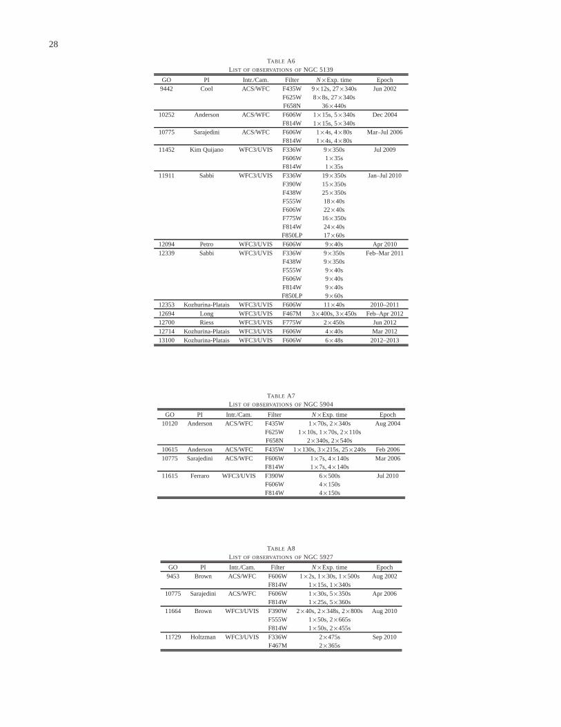
28

TABLE A6L IST OF OBSERVATIONS OFNGC 5139

GO PI Intr./Cam. Filter N×Exp. time Epoch9442 Cool ACS/WFC F435W 9×12s, 27×340s Jun 2002

F625W 8×8s, 27×340sF658N 36×440s

10252 Anderson ACS/WFC F606W 1×15s, 5×340s Dec 2004F814W 1×15s, 5×340s

10775 Sarajedini ACS/WFC F606W 1×4s, 4×80s Mar–Jul 2006F814W 1×4s, 4×80s

11452 Kim Quijano WFC3/UVIS F336W 9×350s Jul 2009F606W 1×35sF814W 1×35s

11911 Sabbi WFC3/UVIS F336W 19×350s Jan–Jul 2010F390W 15×350sF438W 25×350sF555W 18×40sF606W 22×40sF775W 16×350sF814W 24×40sF850LP 17×60s

12094 Petro WFC3/UVIS F606W 9×40s Apr 201012339 Sabbi WFC3/UVIS F336W 9×350s Feb–Mar 2011

F438W 9×350sF555W 9×40sF606W 9×40sF814W 9×40sF850LP 9×60s

12353 Kozhurina-Platais WFC3/UVIS F606W 11×40s 2010–201112694 Long WFC3/UVIS F467M 3×400s, 3×450s Feb–Apr 201212700 Riess WFC3/UVIS F775W 2×450s Jun 201212714 Kozhurina-Platais WFC3/UVIS F606W 4×40s Mar 201213100 Kozhurina-Platais WFC3/UVIS F606W 6×48s 2012–2013

TABLE A7L IST OF OBSERVATIONS OFNGC 5904

GO PI Intr./Cam. Filter N×Exp. time Epoch10120 Anderson ACS/WFC F435W 1×70s, 2×340s Aug 2004

F625W 1×10s, 1×70s, 2×110sF658N 2×340s, 2×540s

10615 Anderson ACS/WFC F435W 1×130s, 3×215s, 25×240s Feb 200610775 Sarajedini ACS/WFC F606W 1×7s, 4×140s Mar 2006

F814W 1×7s, 4×140s11615 Ferraro WFC3/UVIS F390W 6×500s Jul 2010

F606W 4×150sF814W 4×150s

TABLE A8L IST OF OBSERVATIONS OFNGC 5927

GO PI Intr./Cam. Filter N×Exp. time Epoch9453 Brown ACS/WFC F606W 1×2s, 1×30s, 1×500s Aug 2002

F814W 1×15s, 1×340s10775 Sarajedini ACS/WFC F606W 1×30s, 5×350s Apr 2006

F814W 1×25s, 5×360s11664 Brown WFC3/UVIS F390W 2×40s, 2×348s, 2×800s Aug 2010

F555W 1×50s, 2×665sF814W 1×50s, 2×455s

11729 Holtzman WFC3/UVIS F336W 2×475s Sep 2010F467M 2×365s

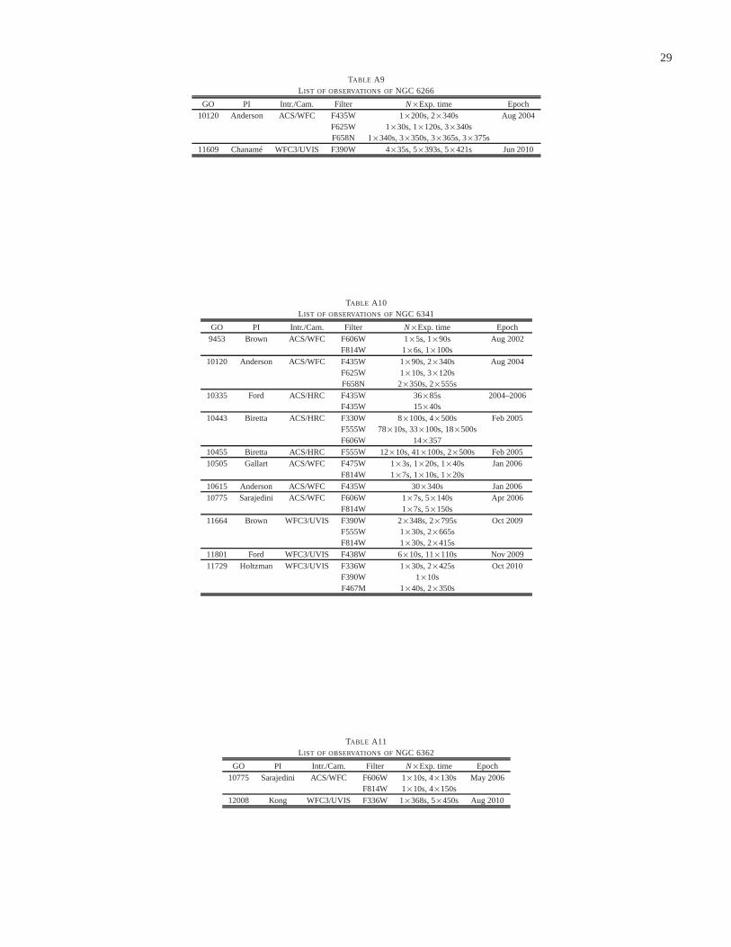
29

TABLE A9L IST OF OBSERVATIONS OFNGC 6266

GO PI Intr./Cam. Filter N×Exp. time Epoch10120 Anderson ACS/WFC F435W 1×200s, 2×340s Aug 2004

F625W 1×30s, 1×120s, 3×340sF658N 1×340s, 3×350s, 3×365s, 3×375s

11609 Chanamé WFC3/UVIS F390W 4×35s, 5×393s, 5×421s Jun 2010

TABLE A10L IST OF OBSERVATIONS OFNGC 6341

GO PI Intr./Cam. Filter N×Exp. time Epoch9453 Brown ACS/WFC F606W 1×5s, 1×90s Aug 2002

F814W 1×6s, 1×100s10120 Anderson ACS/WFC F435W 1×90s, 2×340s Aug 2004

F625W 1×10s, 3×120sF658N 2×350s, 2×555s

10335 Ford ACS/HRC F435W 36×85s 2004–2006F435W 15×40s

10443 Biretta ACS/HRC F330W 8×100s, 4×500s Feb 2005F555W 78×10s, 33×100s, 18×500sF606W 14×357

10455 Biretta ACS/HRC F555W 12×10s, 41×100s, 2×500s Feb 200510505 Gallart ACS/WFC F475W 1×3s, 1×20s, 1×40s Jan 2006

F814W 1×7s, 1×10s, 1×20s10615 Anderson ACS/WFC F435W 30×340s Jan 200610775 Sarajedini ACS/WFC F606W 1×7s, 5×140s Apr 2006

F814W 1×7s, 5×150s11664 Brown WFC3/UVIS F390W 2×348s, 2×795s Oct 2009

F555W 1×30s, 2×665sF814W 1×30s, 2×415s

11801 Ford WFC3/UVIS F438W 6×10s, 11×110s Nov 200911729 Holtzman WFC3/UVIS F336W 1×30s, 2×425s Oct 2010

F390W 1×10sF467M 1×40s, 2×350s

TABLE A11L IST OF OBSERVATIONS OFNGC 6362

GO PI Intr./Cam. Filter N×Exp. time Epoch10775 Sarajedini ACS/WFC F606W 1×10s, 4×130s May 2006

F814W 1×10s, 4×150s12008 Kong WFC3/UVIS F336W 1×368s, 5×450s Aug 2010

30

TABLE A12L IST OF OBSERVATIONS OFNGC 6388

GO PI Intr./Cam. Filter N×Exp. time Epoch9821 Pritzl ACS/WFC F435W 6×11s 2003–2004

F555W 6×7sF814W 6×3s

9835 Drukier ACS/HRC F555W 48×155s Oct 2003F814W 5×25s, 2×469s, 10×505s

10350 Cohn ACS/HRC F330W 2×1266s, 4×1314s Apr 2006F555W 3×155s

10474 Drukier ACS/HRC F555W 48×155s Apr 2006F814W 4×25s, 8×501s, 4×508s

10775 Sarajedini ACS/WFC F606W 1×40s, 5×340s Apr 2006F814W 1×40s, 5×350s

11739 Piotto WFC3/UVIS F390W 6×880s Jun–Jul 2010

TABLE A13L IST OF OBSERVATIONS OFNGC 6397

GO PI Intr./Cam. Filter N×Exp. time Epoch10257 Anderson ACS/WFC F435W 5×13s, 5×340s 2004–2005

F625W 5×10s, 5×340sF658N 20×390s, 20×395s

10775 Sarajedini ACS/WFC F606W 1×1s, 4×15s May 2006F814W 1×1s, 4×15s

11633 Rich WFC3/UVIS F336W 6×620s Mar 2010F606W 6×360s

TABLE A14L IST OF OBSERVATIONS OFNGC 6441

GO PI Intr./Cam. Filter N×Exp. time Epoch9835 Drukier ACS/HRC F555W 36×240s Sep 2003

F814W 5×40s, 2×413s, 10×440s10775 Sarajedini ACS/WFC F606W 1×45s, 5×340s May 2006

F814W 1×45s, 5×350s11739 Piotto WFC3/UVIS F390W 2×880s, 2×884s, 8×885s 2010–2011

TABLE A15L IST OF OBSERVATIONS OFNGC 6535

GO PI Intr./Cam. Filter N×Exp. time Epoch10775 Sarajedini ACS/WFC F606W 1×12s, 4×130s Mar 2006

F814W 1×12s, 4×150s12008 Kong ACS/WFC F625W 1×100s, 1×148s Sep 2010

F658N 1×588s, 1×600sWFC3/UVIS F336W 1×253s, 5×400s

TABLE A16L IST OF OBSERVATIONS OFNGC 6624

GO PI Intr./Cam. Filter N×Exp. time Epoch10401 Chandar ACS/HRC F435W 20×200s Feb 200510775 Sarajedini ACS/WFC F606W 1×15s, 5×350s Apr 2006

F814W 1×15s, 5×350s10573 Mateo ACS/WFC F435W 1×360s Jun 2006

F555W 1×160sF814W 1×65s

31

TABLE A17L IST OF OBSERVATIONS OFNGC 6656

GO PI Intr./Cam. Filter N×Exp. time Epoch10775 Sarajedini ACS/WFC F606W 1×3s, 4×55s Apr 2006

F814W 1×3s, 4×65s11558 De Marco ACS/WFC F502N 2×441s, 1×2102x, 1×2322s Mar 201012311 Piotto WFC3/UVIS F814W 4×50s 2010–2011

TABLE A18L IST OF OBSERVATIONS OFNGC 6681

GO PI Intr./Cam. Filter N×Exp. time Epoch9019 Bohlin ACS/HRC F330W 4×170s Apr 20029010 Tran ACS/HRC F330W 6×70s May–June 20029565 De Marchi ACS/HRC F330W 16×70s Jun-Sep 20029566 De Marchi ACS/HRC F330W 17×70s Feb 20039655 Giavalisco ACS/HRC F330W 16×70s Feb–Sep 200310047 Giavalisco ACS/HRC F330W 6×70s Mar–Sep 200410401 Chandar ACS/HRC F435W 26×125s Feb 200510373 Giavalisco ACS/HRC F330W 4×70s 2005–200610736 Maiz-Apellaniz ACS/HRC F330W 8×20s Mar 2006

F435W 4×2sF555W 4×2sF625W 4×1sF814W 4×1s

10775 Sarajedini ACS/WFC F606W 1×10s, 4×140s May 2006F814W 1×10s, 4×150s

12516 Ferraro WFC3/UVIS F390W 12×348s Nov 2011F555W 2×127s, 8×150sF814W 13×348s

TABLE A19L IST OF OBSERVATIONS OFNGC 6752

GO PI Intr./Cam. Filter N×Exp. time Epoch9453 Brown ACS/WFC F606W 1×4s, 1×40s Sep 2002

F814W 1×4s, 1×45s9899 Piotto ACS/WFC F475W 6×340s Jul 200410121 Bailyn ACS/WFC F555W 12×80s, 11×435s Sep 2004

F814W 12×40s10335 Ford ACS/HRC F435W 24×35s 2004–2006

F555W 13×10s10458 Biretta ACS/HRC F555W 12×10s, 4×100s, 2×500s Aug 2005

F606W 2×357s10459 Biretta ACS/WFC F606W 8×450 Oct 200510335 Ford ACS/HRC F435W 24×35s Jun 2004

F555W 13×10s10775 Sarajedini ACS/WFC F606W 1×2s, 4×35s May 2006

F814W 1×2s, 4×40s11801 Ford WFC3/UVIS F438W 4×5s, 18×45s Nov 200911664 Brown WFC3/UVIS F390W 2×348s, 2×880s May 2010

F555W 1×30s, 2×665sF814W 1×30s, 2×495s

11904 Kalirai WFC3/UVIS F555W 15×550s Jul–Aug 2010F814W 15×550s

12254 Cool ACS/WFC F435W 6×10s, 12×380s May–Nov 2011F625W 18×10s, 12×360sF658N 12×724s, 12×820s

12311 Piotto WFC3/UVIS F814W 2×50s Mar–Apr 2011

TABLE A20L IST OF OBSERVATIONS OFNGC 6715

GO PI Intr./Cam. Filter N×Exp. time Epoch10775 Sarajedini ACS/WFC F606W 2×30s, 10×340s May 2006

F814W 2×30s, 10×350s12274 van der Marel WFC3/UVIS F438W 10×30s, 5×234s, 5×256s Sep 2011

32

TABLE A21L IST OF OBSERVATIONS OFNGC 7078

GO PI Intr./Cam. Filter N×Exp. time Epoch10401 Chandar ACS/HRC F435W 13×125s Dec 200410775 Sarajedini ACS/WFC F606W 1×15s, 4×130s May 2006

F814W 1×15s, 4×150s11233 Piotto WFC3/UVIS F390W 6×827s May 201012605 Piotto WFC3/UVIS F336W 6×350s Oct 2011

F438W 6×65s

TABLE A22L IST OF OBSERVATIONS OFNGC 7099

GO PI Intr./Cam. Filter N×Exp. time Epoch10401 Chandar ACS/HRC F435W 13×125s Dec 200410775 Sarajedini ACS/WFC F606W 1×7s, 4×140s May 2006

F814W 1×7s, 4×140s

33

APPENDIX B. PROPER-MOTION CATALOG OF NGC 7078

Our procedures generate a large number of parameters for each star, but most users will need only the high-level data. ThePMcatalog of NGC 7078 contains 91 lines of header information,followed by one line for each star with a PM measurement, for atotal of 77837 stars. Stars in the catalog are sorted according to their distance from the cluster center, as given in Table 1.

The header starts with some general information about the cluster, such as the reference time of the master frame and theadopted cluster center position, in both equatorial and master-frame units. Then follows a column-by-column description of thecatalog. The columns contain: the reference-frame positions and distance from the cluster center, calibrated and differential-reddening-corrected F606W and F814W magnitudes with errors and some photometric-quality information, PMs with errorsderived using both the expected errors as a weight and the actual residuals around the PM least-squares fits (see Section 6.1,some additional astrometric-quality information, and finally the differences between local-corrected and amplifier-based PMs(see Section 7.4). A description of each column of the catalog is given in Table B1, while the first 10 lines of the NGC 7078 PMcatalog are shown in Table B2.

TABLE B1COLUMN-BY-COLUMN INFORMATION CONTAINED IN THE CATALOG

Col Name (unit) ExplanationAstrometric information

1 r (′′) Distance from the cluster center2 ∆x0 (′′) GO-10775 x-position in the rectified Cartesian system withrespect to the adopted center3 ∆y0 (′′) GO-10775 y-position in the rectified Cartesian system withrespect to the adopted center4 µα cosδ (masyr−1) PM along the x axis (parallel to and increasing as R.A.)5 µδ (mas yr−1) PM along the y axis (parallel to and increasing as Dec.)6 σµα cosδ (masyr−1) 1-σ uncertainty inµα cosδ computed using actual residuals7 σµδ

(mas yr−1) 1-σ uncertainty inµδ computed using actual residuals8 xM (pixel) x-position on the master frame9 yM (pixel) y-position on the master frame10 ∆x (pixel) difference betweenxM and the PM-predicted position at the reference time (x)11 ∆y (pixel) difference betweenyM and the PM-predicted position at the reference time (y)12 errµα cosδ (masyr−1) 1-σ uncertainty inµα cosδ computed using expected errors13 errµδ

(mas yr−1) 1-σ uncertainty inµδ computed using expected errors

Photometric information14 mF606W (mag) Differential-reddening-corrected GO-10775 F606W Vega-mag photometry15 mF814W (mag) Differential-reddening-corrected GO-10775 F814W Vega-mag photometry16 σmF606W (mag) Photometric error in F606W (from GO-10775)17 σmF814W (mag) Photometric error in F814W (from GO-10775)18 QFITF606W Quality of F606W PSF-fit (from GO-10775)19 QFITF814W Quality of F814W PSF-fit (from GO-10775)

Proper-motion quality information20 χ2

µα cosδ Reducedχ2 of the fit of the x-component of the motion

21 χ2µδ

Reducedχ2 of the fit of the y-component of the motion

22 σx (pix) 1-σ uncertainty in the intercept of the PM fit for the x-componentusing actual residuals23 σy (pix) 1-σ uncertainty in the intercept of the PM fit for the y-componentusing actual residuals24 time (yr) Time baseline, in Julian years25 errx (pix) 1-σ uncertainty in the intercept of the PM fit for the x-componentusing expected errors26 erry (pix) 1-σ uncertainty in the intercept of the PM fit for the y-componentusing expected errors27 Uref Flag: 1 if used as reference bona-fide cluster star for the linear transformations, 0 otherwise28 Nfound Initial number of data points for the PM fits29 Nused Final number of data points used for the PM fits30 ID ID number for each star (not the GO-10775 ID)

Local PM corrections31 ∆µα cosδ (masyr−1) Difference inµα cosδ between locally-corrected and amplifier-based PMs. Add to column 4

to obtain locally-corrected PMs.32 ∆µδ (masyr−1) Difference inµδ between locally-corrected and amplifier-based PMs. Add to column 5 to

obtain locally-corrected PMs.

34

TABLE B2FIRST TEN LINES OF THENGC 7078 PMCATALOG

r (′′) ∆x0 (′′) ∆y0 (′′) µα cosδ µδ σµα cosδ σµδxM yM ∆x ∆y errµα cosδ errµδ

mF606W mF814W σmF606W →

(1) (2) (3) (4) (5) (6) (7) (8) (9) (10) (11) (12) (13) (14) (15) (16)0.22148 0.19883 0.09756 −0.203 0.249 0.039 0.030 4984.312 5019.940 0.024 0.014 0.0320.030 17.015 16.276 9.900 . . .0.50339 0.24141 0.44172 −3.057 9.266 0.367 2.021 4983.246 5028.540−0.078 −0.241 0.418 0.957 18.253 17.774 9.900 . . .1.13357 0.84530 0.75528 0.201 0.245 0.045 0.054 4968.149 5036.379 0.030 0.003 0.042 0.037 15.508 15.113 9.900 . . .1.24526 1.18454 0.38412 −0.283 0.055 0.020 0.038 4959.674 5027.097−0.014 0.052 0.021 0.034 15.985 15.801 9.900 . . .1.32849 0.86993 1.00404 0.001 −0.192 0.023 0.021 4967.535 5042.601 0.012−0.008 0.024 0.018 16.974 16.193 9.900 . . .1.33293 0.59227 1.19412 0.321 −0.101 0.027 0.031 4974.479 5047.344 0.004−0.013 0.027 0.035 17.419 16.724 9.900 . . .1.46104 −1.44918 0.18576 0.176 −0.084 0.022 0.023 5025.506 5022.140 0.016 0.012 0.018 0.02816.686 15.977 9.900 . . .1.62112 −0.24352 1.60272 0.054 −0.045 0.034 0.019 4995.371 5057.557−0.030 0.022 0.029 0.023 15.478 15.406 9.900 . . .1.77721 −1.39604 −1.09980 −0.403 0.109 0.025 0.046 5024.188 4990.005 0.022 0.005 0.0240.036 17.375 16.719 9.900 . . .1.90239 −1.31299 1.37664 0.387 −0.474 0.015 0.031 5022.109 5051.913 0.021−0.021 0.019 0.029 17.443 16.765 9.900 . . .

. . . . . . . . . . . . . . . . . . . . . . . . . . . . . . . . . . . . . . . . . . . . . . . . . . .→ σmF814W QFITF606W QFITF814W χ2

µα cosδ χ2µδ

σx σy time errx erry Uref Nfound Nused ID ∆µα cosδ ∆µδ

(17) (18) (19) (20) (21) (22) (23) (24) (25) (26) (27) (28) (29) (30) (31) (32). . . 9.900 0.080 0.056 2.412 2.116 0.0018 0.0017 6.96206 0.0018 0.0016 1 30 24 86023 0.004 0.005. . . 9.900 0.331 0.347 2.328 11.882 0.0134 0.0749 1.48741 0.0153 0.0350 0 26 15 86021 0.023 −0.079. . . 9.900 0.084 0.049 3.502 2.750 0.0020 0.0022 6.96206 0.0019 0.0017 0 20 18 86020 0.047 0.013. . . 9.900 0.062 0.043 1.706 4.652 0.0011 0.0019 6.96206 0.0011 0.0018 0 25 23 86022 0.049 0.014. . . 9.900 0.118 0.063 1.279 0.796 0.0014 0.0011 6.96206 0.0013 0.0010 1 24 21 86019 0.017 −0.002. . . 9.900 0.115 0.117 1.475 2.553 0.0016 0.0021 6.96206 0.0015 0.0020 1 25 23 86018 −0.006 0.017. . . 9.900 0.080 0.084 1.045 2.306 0.0010 0.0017 6.96206 0.0010 0.0016 1 27 26 86483 0.022 −0.028. . . 9.900 0.046 0.042 1.746 1.067 0.0015 0.0011 6.96195 0.0014 0.0011 0 16 14 86228 0.033 0.001. . . 9.900 0.098 0.068 1.140 2.624 0.0013 0.0020 6.96206 0.0013 0.0021 1 25 25 86481 −0.010 0.011. . . 9.900 0.146 0.096 0.895 2.024 0.0013 0.0016 6.96206 0.0012 0.0018 1 27 26 86485 −0.010 0.005. . . . . . . . . . . . . . . . . . . . . . . . . . . . . . . . . . . . . . . . . . . . . . . . . . .