A beginner's tutorial for MASA-FEMAP FOR ANALYSIS OF ...
151
A beginner’s tutorial for MASA-FEMAP FOR ANALYSIS OF CONCRETE AND REINFORCED CONCRETE STRUCTURAL ELEMENTS By Akanshu Sharma Visiting Researcher from Bhabha Atomic Research Centre, Mumbai, India Institut für Werkstoffe im Bauwesen, Universität Stuttgart, Germany August 2010, rev April 2012 Institute of Construction Materials Fastening Technology Department University of Stuttgart Pfaffenwaldring 4 70569 Stuttgart, Germany
Transcript of A beginner's tutorial for MASA-FEMAP FOR ANALYSIS OF ...

A beginner’s tutorial for
MASA-FEMAP FOR ANALYSIS OF CONCRETE AND REINFORCED
CONCRETE STRUCTURAL ELEMENTS
By
Akanshu Sharma
Visiting Researcher from Bhabha Atomic Research Centre, Mumbai, India
Institut für Werkstoffe im Bauwesen,
Universität Stuttgart, Germany
August 2010, rev April 2012
Institute of Construction Materials
Fastening Technology Department
University of Stuttgart
Pfaffenwaldring 4
70569 Stuttgart, Germany

DISCLAIMER (PLEASE READ)
This tutorial is made to the best of knowledge and belief of the author at the time of making
this tutorial. However, it is not claimed by the author that the tutorial is error free. In case of
any doubt, the reader may contact the author or other users of MASA and FEMAP.
In case you should find any errors or you want to improve this tutorial, please send an
email to: [email protected] or [email protected]
stuttgart.de.
This tutorial is in no way intended to provide any technical details of MASA or FEMAP but
is intended to give the beginners of MASA a platform to begin with. The tutorial also does not
cover any wide range of problems but it gives sufficient information about modelling and
handling problems related to structural elements. It is believed that after going through this
tutorial, one may be in a position to carry on further with problems with various levels of
difficulty.
Also, since this tutorial is made only to teach to the people beginning with MASA and
FEMAP about how to work with MASA and FEMAP, the mesh sizes and steps are generally
kept coarse so as to save time. However, a person can always try to refine the mesh and get
better results.
In the same folder as the tutorial you will find all the input files required to start an analysis.
The stcw solver used to analyze the examples is attached as well.

TUTORIAL 1
ANALYSIS OF SIMPLY SUPPORTED RECTANGULAR CONCRETE BEAM UNDER THREE POINT BENDING
(Input files available under name :example1.ms3)
In this tutorial, you will learn
1. Basic modeling of solids
2. Application of load
3. Application of end conditions
4. Giving input for material properties
5. Visualizing the results
Statement of Problem
To analyze a simply supported plain concrete (un-reinforced) beam with rectangular cross-section subjected to a concentrated load on the mid-span. The dimensions for the beam are given in Figure below.
The following material properties shall be used for analysis:
Compressive strength of concrete = 25 MPa
Tensile strength of concrete = 2.5 MPa
Elastic Modulus of concrete = 25000 MPa
Poisson’s Ratio = 0.18
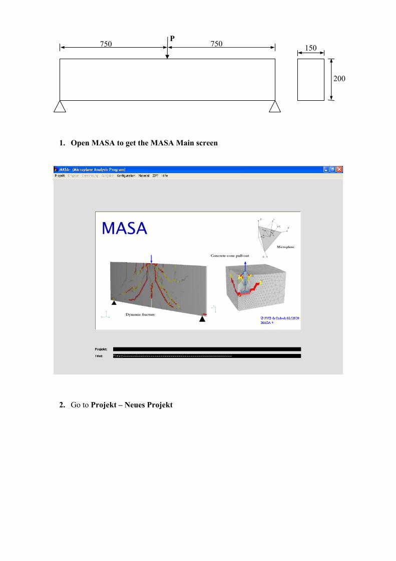
1. Open MASA to get the MASA Main screen
2. Go to Projekt – Neues Projekt
750 750P
150
200
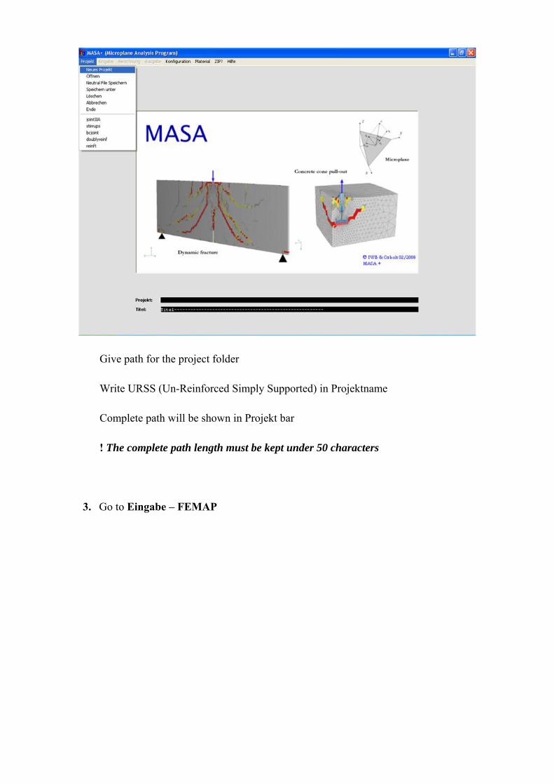
Give path for the project folder Write URSS (Un-Reinforced Simply Supported) in Projektname Complete path will be shown in Projekt bar ! The complete path length must be kept under 50 characters
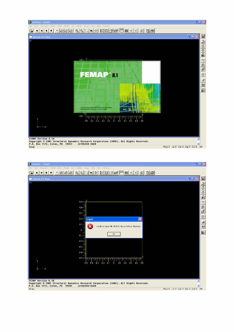
3. Go to Eingabe – FEMAP
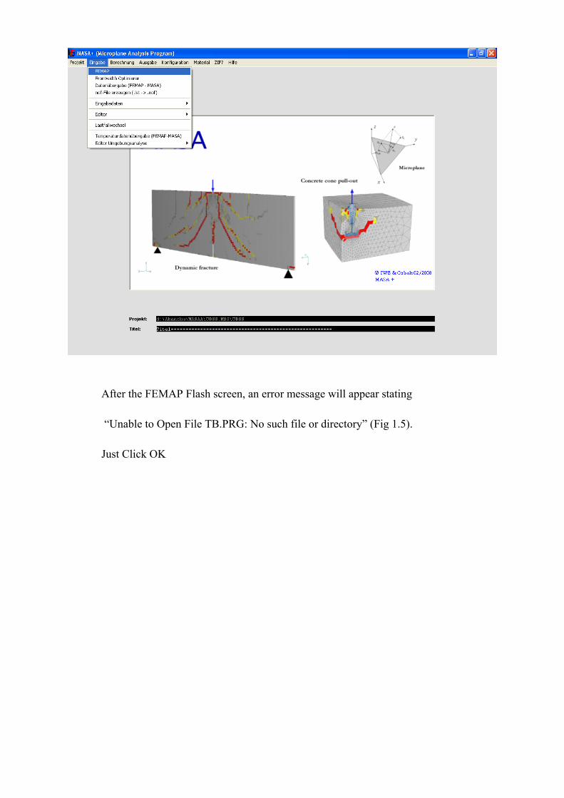
After the FEMAP Flash screen, an error message will appear stating “Unable to Open File TB.PRG: No such file or directory” (Fig 1.5). Just Click OK
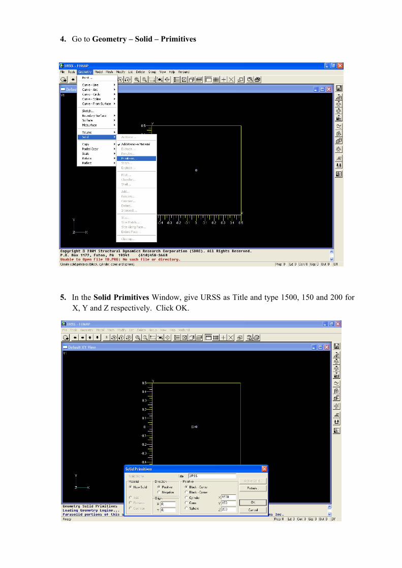
4. Go to Geometry – Solid – Primitives
5. In the Solid Primitives Window, give URSS as Title and type 1500, 150 and 200 for X, Y and Z respectively. Click OK.
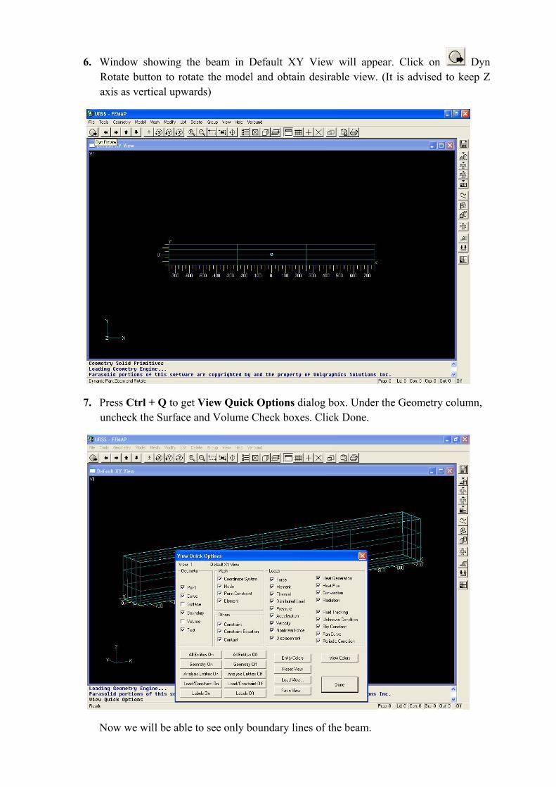
6. Window showing the beam in Default XY View will appear. Click on Dyn Rotate button to rotate the model and obtain desirable view. (It is advised to keep Z axis as vertical upwards)
7. Press Ctrl + Q to get View Quick Options dialog box. Under the Geometry column, uncheck the Surface and Volume Check boxes. Click Done.
Now we will be able to see only boundary lines of the beam.
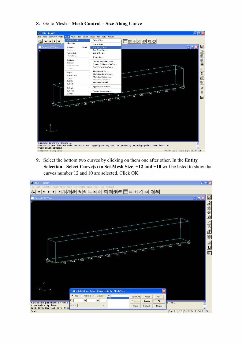
8. Go to Mesh – Mesh Control – Size Along Curve
9. Select the bottom two curves by clicking on them one after other. In the Entity Selection - Select Curve(s) to Set Mesh Size, +12 and +10 will be listed to show that curves number 12 and 10 are selected. Click OK.
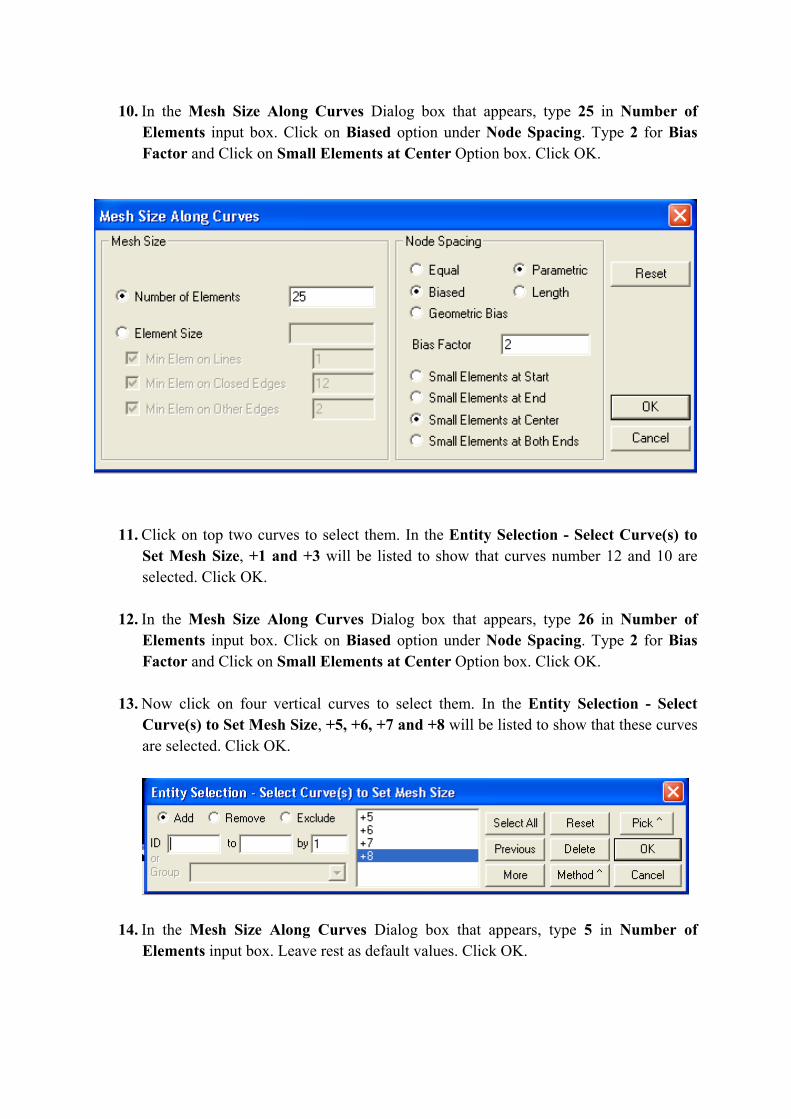
10. In the Mesh Size Along Curves Dialog box that appears, type 25 in Number of Elements input box. Click on Biased option under Node Spacing. Type 2 for Bias Factor and Click on Small Elements at Center Option box. Click OK.
11. Click on top two curves to select them. In the Entity Selection - Select Curve(s) to Set Mesh Size, +1 and +3 will be listed to show that curves number 12 and 10 are selected. Click OK.
12. In the Mesh Size Along Curves Dialog box that appears, type 26 in Number of Elements input box. Click on Biased option under Node Spacing. Type 2 for Bias Factor and Click on Small Elements at Center Option box. Click OK.
13. Now click on four vertical curves to select them. In the Entity Selection - Select Curve(s) to Set Mesh Size, +5, +6, +7 and +8 will be listed to show that these curves are selected. Click OK.
14. In the Mesh Size Along Curves Dialog box that appears, type 5 in Number of Elements input box. Leave rest as default values. Click OK.
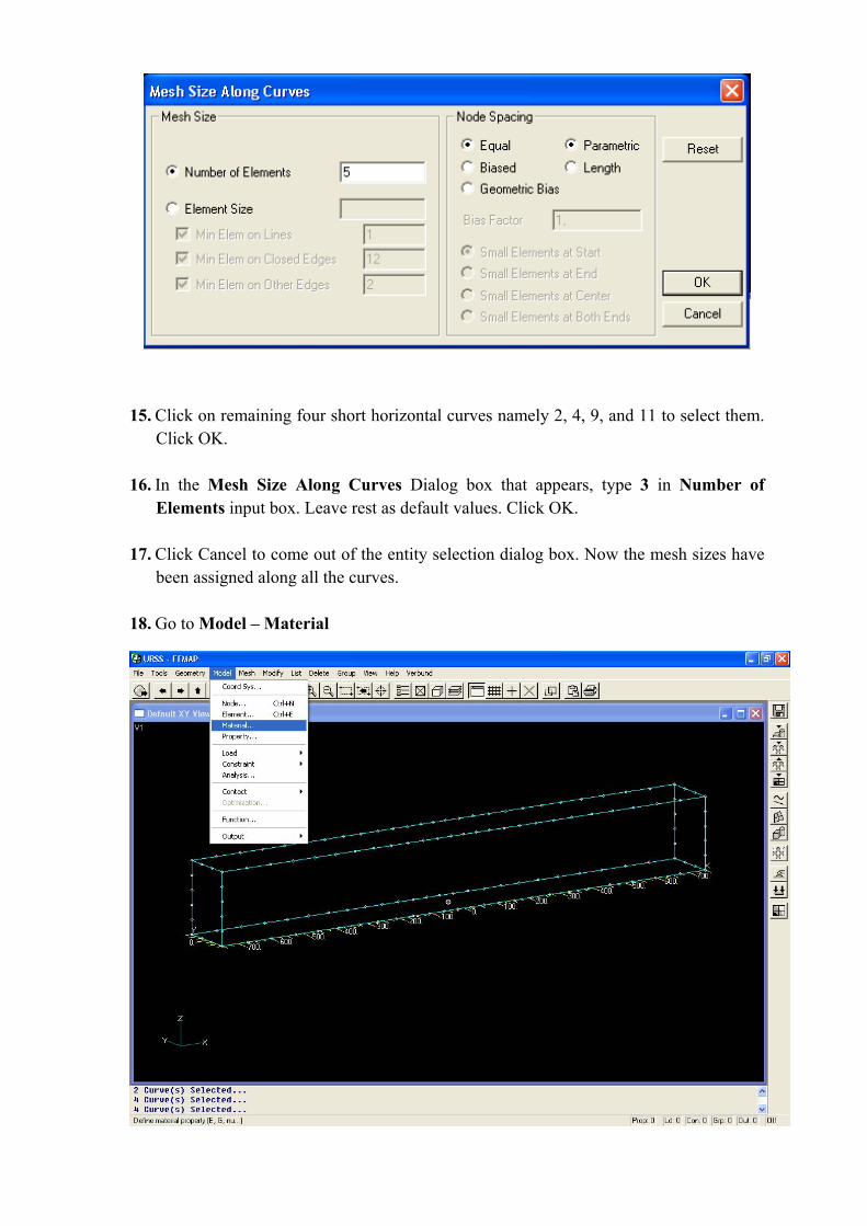
15. Click on remaining four short horizontal curves namely 2, 4, 9, and 11 to select them. Click OK.
16. In the Mesh Size Along Curves Dialog box that appears, type 3 in Number of Elements input box. Leave rest as default values. Click OK.
17. Click Cancel to come out of the entity selection dialog box. Now the mesh sizes have been assigned along all the curves.
18. Go to Model – Material
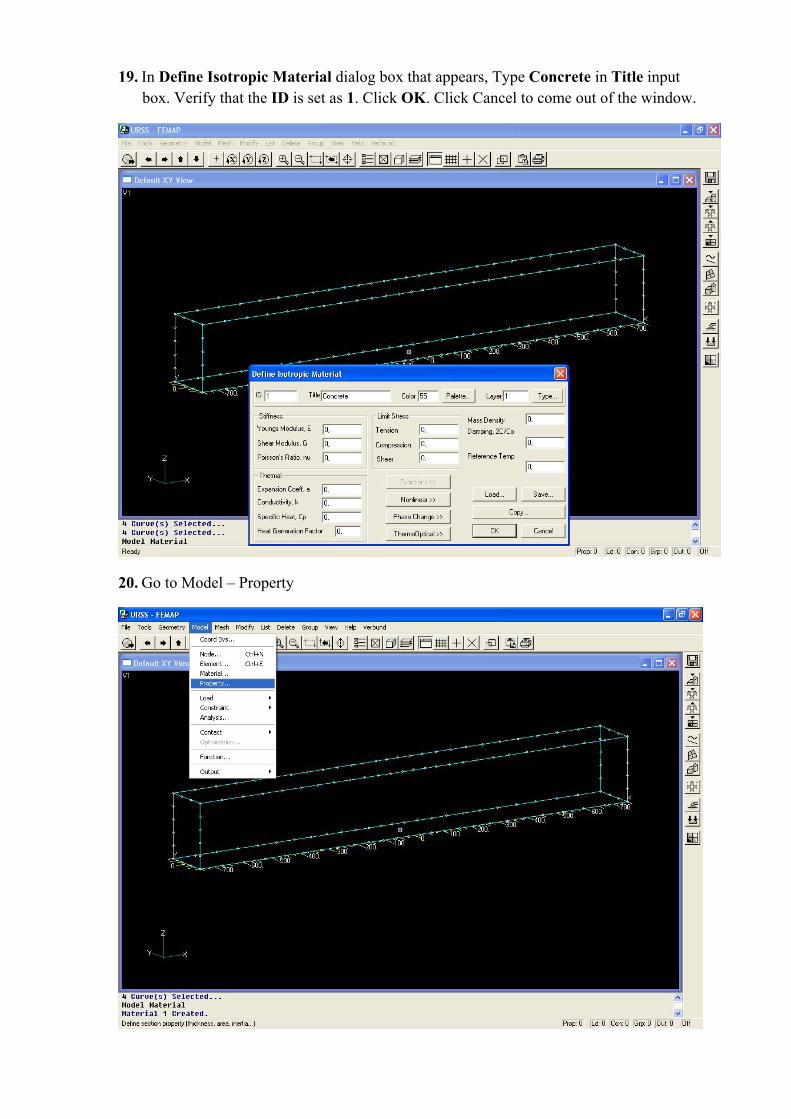
19. In Define Isotropic Material dialog box that appears, Type Concrete in Title input box. Verify that the ID is set as 1. Click OK. Click Cancel to come out of the window.
20. Go to Model – Property
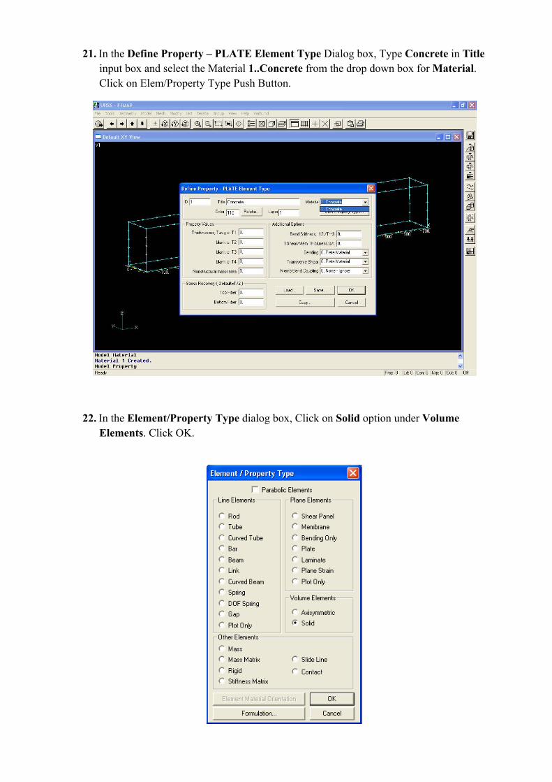
21. In the Define Property – PLATE Element Type Dialog box, Type Concrete in Title input box and select the Material 1..Concrete from the drop down box for Material. Click on Elem/Property Type Push Button.
22. In the Element/Property Type dialog box, Click on Solid option under Volume Elements. Click OK.
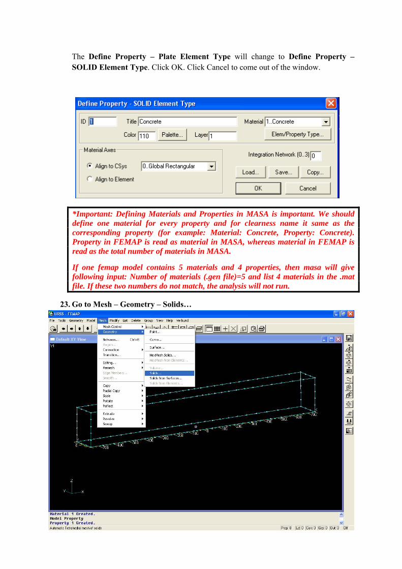
The Define Property – Plate Element Type will change to Define Property – SOLID Element Type. Click OK. Click Cancel to come out of the window.
*Important: Defining Materials and Properties in MASA is important. We should define one material for every property and for clearness name it same as the corresponding property (for example: Material: Concrete, Property: Concrete). Property in FEMAP is read as material in MASA, whereas material in FEMAP is read as the total number of materials in MASA.
If one femap model contains 5 materials and 4 properties, then masa will give following input: Number of materials (.gen file)=5 and list 4 materials in the .mat file. If these two numbers do not match, the analysis will not run.
23. Go to Mesh – Geometry – Solids…
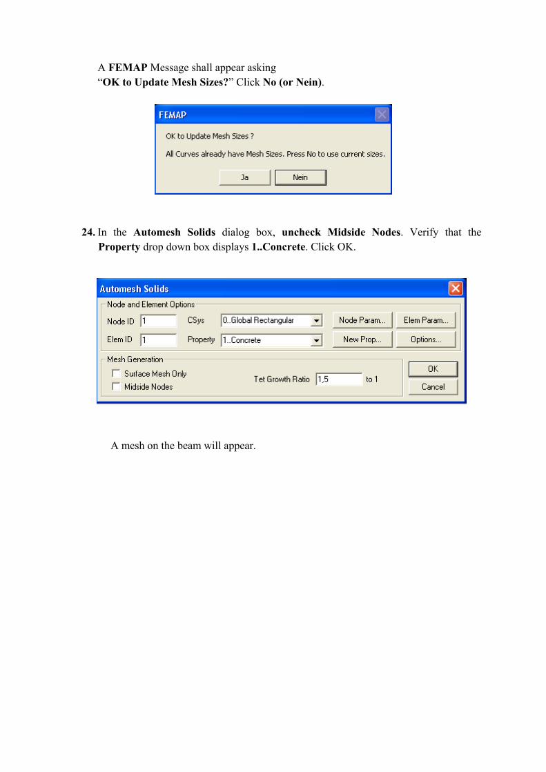
A FEMAP Message shall appear asking “OK to Update Mesh Sizes?” Click No (or Nein).
24. In the Automesh Solids dialog box, uncheck Midside Nodes. Verify that the
Property drop down box displays 1..Concrete. Click OK.
A mesh on the beam will appear.
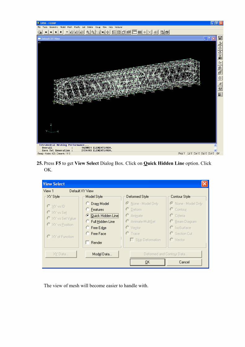
25. Press F5 to get View Select Dialog Box. Click on Quick Hidden Line option. Click OK.
The view of mesh will become easier to handle with.
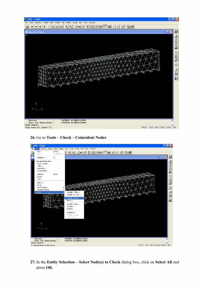
26. Go to Tools – Check – Coincident Nodes
27. In the Entity Selection – Select Node(s) to Check dialog box, click on Select All and press OK.
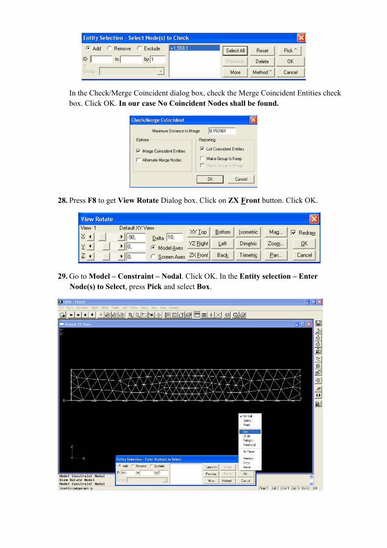
In the Check/Merge Coincident dialog box, check the Merge Coincident Entities check box. Click OK. In our case No Coincident Nodes shall be found.
28. Press F8 to get View Rotate Dialog box. Click on ZX Front button. Click OK.
29. Go to Model – Constraint – Nodal. Click OK. In the Entity selection – Enter Node(s) to Select, press Pick and select Box.
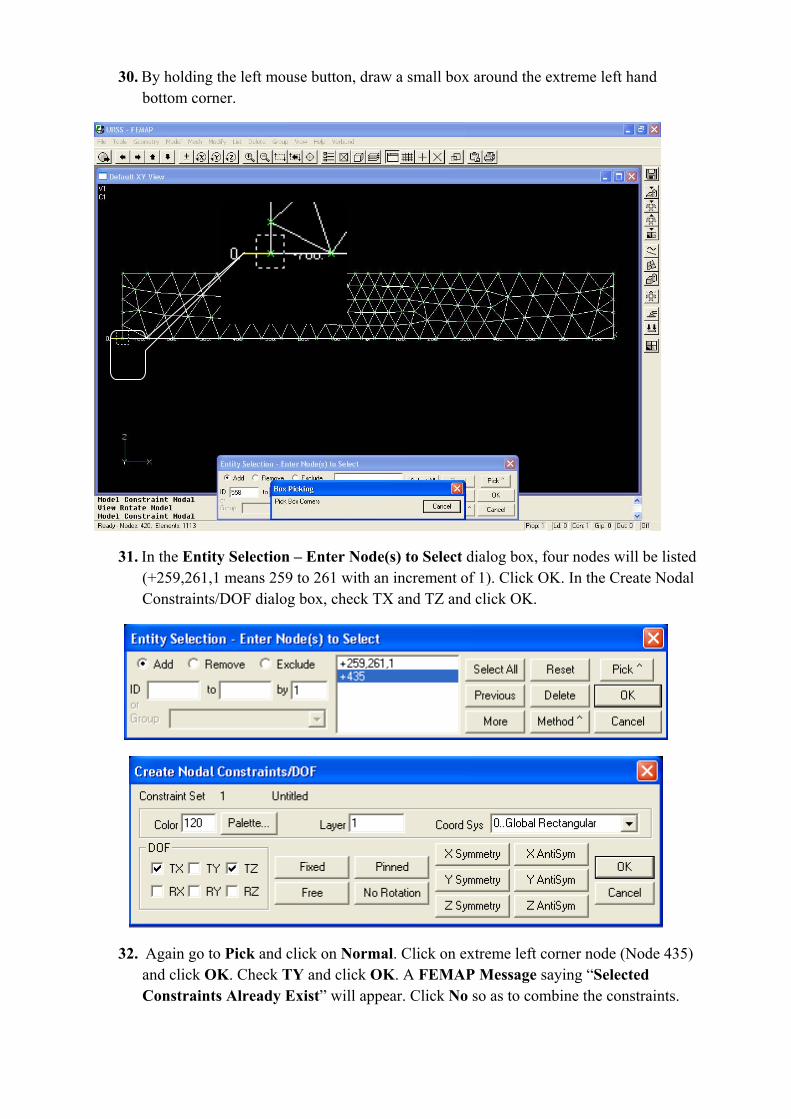
30. By holding the left mouse button, draw a small box around the extreme left hand bottom corner.
31. In the Entity Selection – Enter Node(s) to Select dialog box, four nodes will be listed (+259,261,1 means 259 to 261 with an increment of 1). Click OK. In the Create Nodal Constraints/DOF dialog box, check TX and TZ and click OK.
32. Again go to Pick and click on Normal. Click on extreme left corner node (Node 435) and click OK. Check TY and click OK. A FEMAP Message saying “Selected Constraints Already Exist” will appear. Click No so as to combine the constraints.
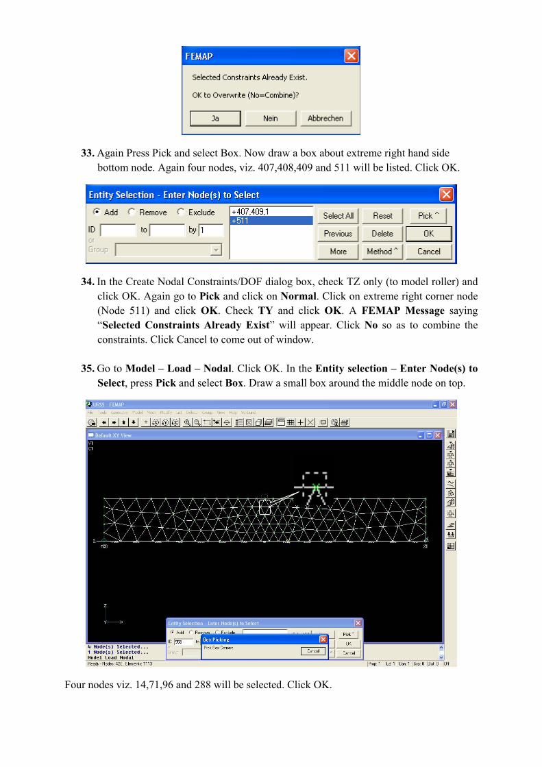
33. Again Press Pick and select Box. Now draw a box about extreme right hand side bottom node. Again four nodes, viz. 407,408,409 and 511 will be listed. Click OK.
34. In the Create Nodal Constraints/DOF dialog box, check TZ only (to model roller) and click OK. Again go to Pick and click on Normal. Click on extreme right corner node (Node 511) and click OK. Check TY and click OK. A FEMAP Message saying “Selected Constraints Already Exist” will appear. Click No so as to combine the constraints. Click Cancel to come out of window.
35. Go to Model – Load – Nodal. Click OK. In the Entity selection – Enter Node(s) to Select, press Pick and select Box. Draw a small box around the middle node on top.
Four nodes viz. 14,71,96 and 288 will be selected. Click OK.
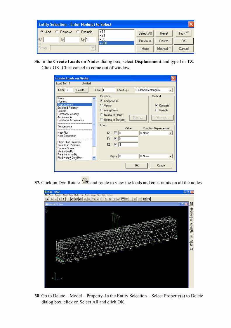
36. In the Create Loads on Nodes dialog box, select Displacement and type 1in TZ. Click OK. Click cancel to come out of window.
37. Click on Dyn Rotate and rotate to view the loads and constraints on all the nodes.
38. Go to Delete – Model – Property. In the Entity Selection – Select Property(s) to Delete dialog box, click on Select All and click OK.
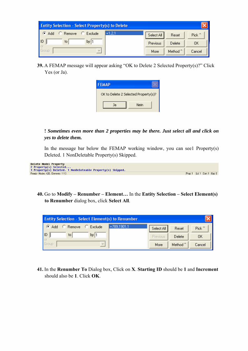
39. A FEMAP message will appear asking “OK to Delete 2 Selected Property(s)?” Click Yes (or Ja).
! Sometimes even more than 2 properties may be there. Just select all and click on yes to delete them.
In the message bar below the FEMAP working window, you can see1 Property(s) Deleted. 1 NonDeletable Property(s) Skipped.
40. Go to Modify – Renumber – Element… In the Entity Selection – Select Element(s) to Renumber dialog box, click Select All.
41. In the Renumber To Dialog box, Click on X. Starting ID should be 1 and Increment should also be 1. Click OK.
42. Go to Modify – Renumber – Node… In the Entity Selection – Select Node(s) to Renumber dialog box, click Select All.
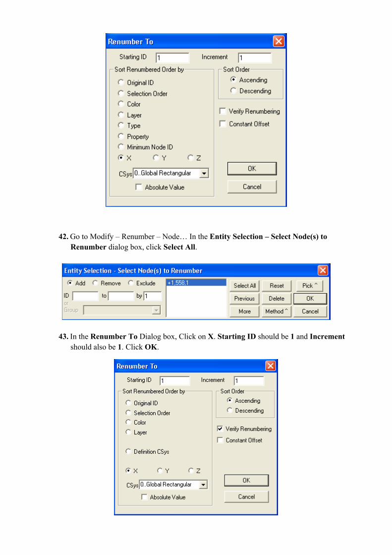
43. In the Renumber To Dialog box, Click on X. Starting ID should be 1 and Increment should also be 1. Click OK.
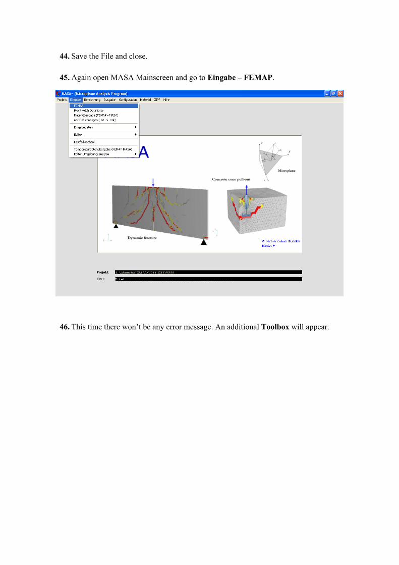
44. Save the File and close. 45. Again open MASA Mainscreen and go to Eingabe – FEMAP.
46. This time there won’t be any error message. An additional Toolbox will appear.
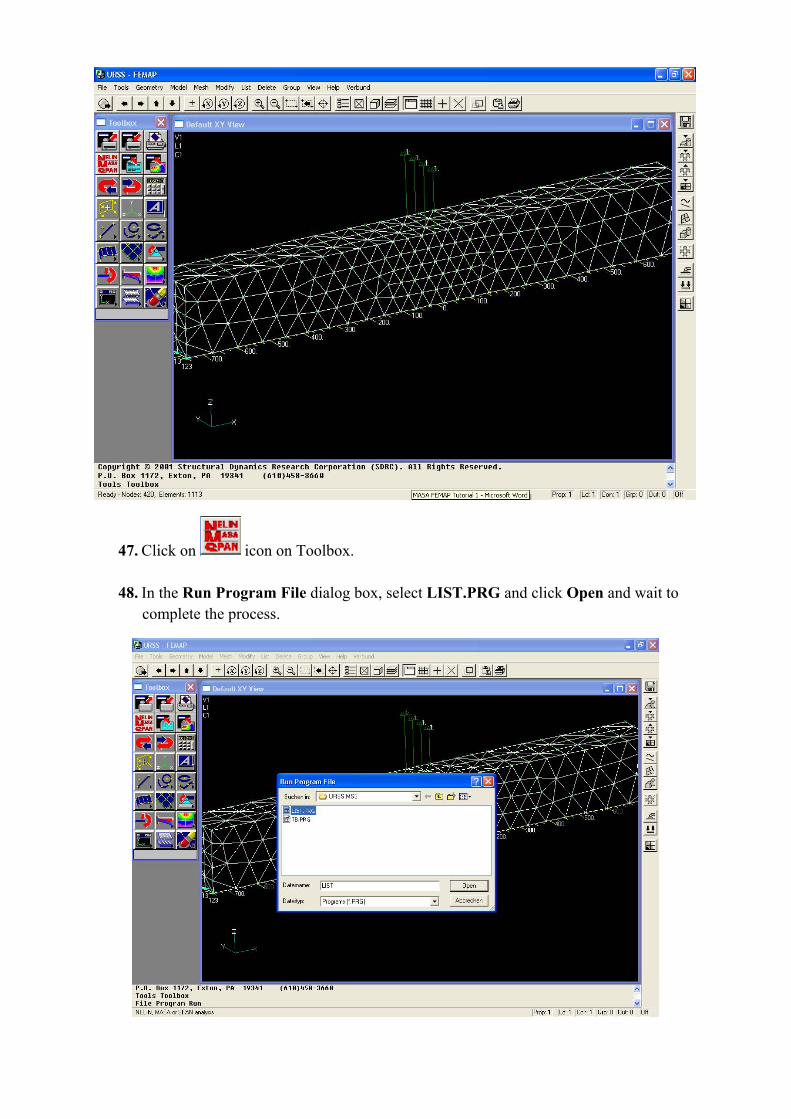
47. Click on icon on Toolbox.
48. In the Run Program File dialog box, select LIST.PRG and click Open and wait to complete the process.
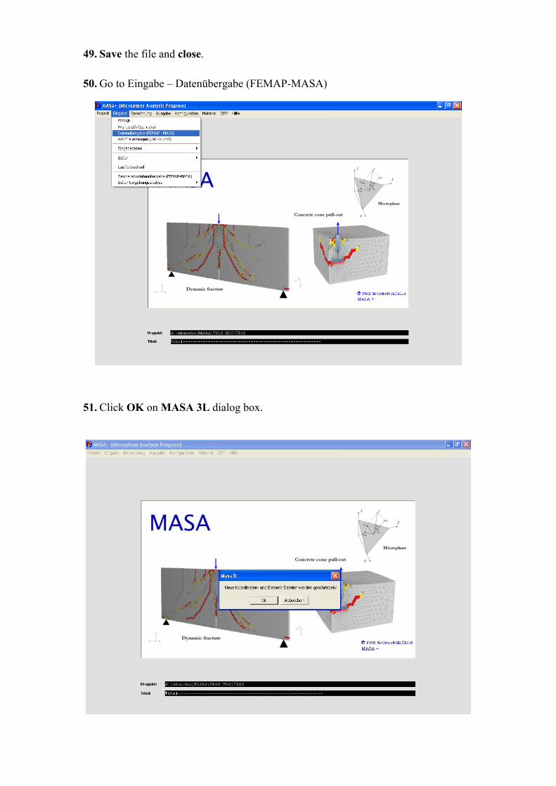
49. Save the file and close.
50. Go to Eingabe – Datenübergabe (FEMAP-MASA)
51. Click OK on MASA 3L dialog box.
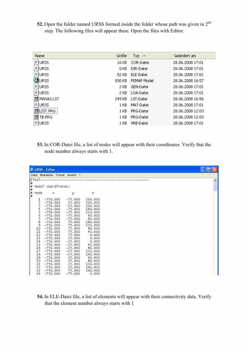
52. Open the folder named URSS formed inside the folder whose path was given in 2nd step. The following files will appear there. Open the files with Editor.
53. In COR-Datei file, a list of nodes will appear with their coordinates. Verify that the node number always starts with 1.
54. In ELE-Datei file, a list of elements will appear with their connectivity data. Verify that the element number always starts with 1
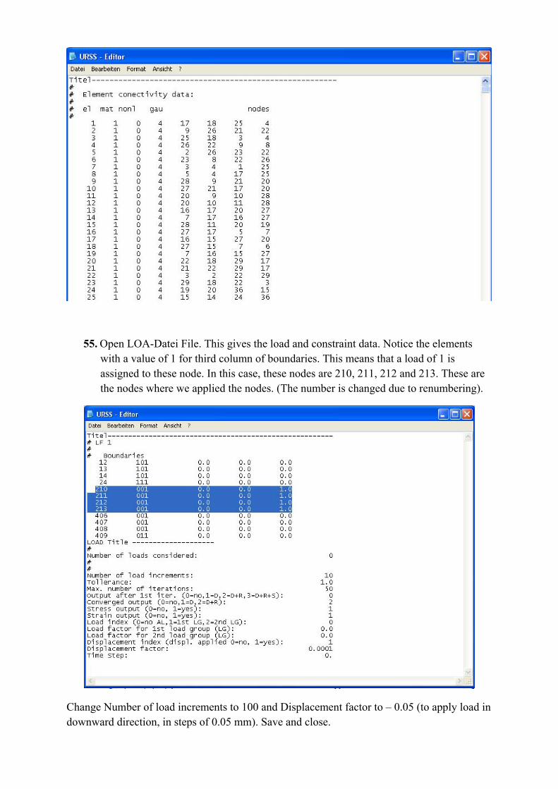
55. Open LOA-Datei File. This gives the load and constraint data. Notice the elements with a value of 1 for third column of boundaries. This means that a load of 1 is assigned to these node. In this case, these nodes are 210, 211, 212 and 213. These are the nodes where we applied the nodes. (The number is changed due to renumbering).
Change Number of load increments to 100 and Displacement factor to – 0.05 (to apply load in downward direction, in steps of 0.05 mm). Save and close.
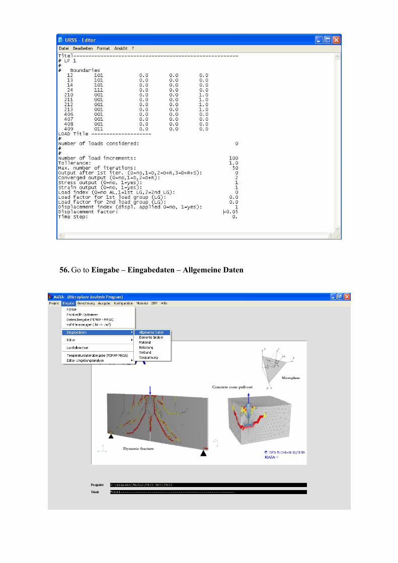
56. Go to Eingabe – Eingabedaten – Allgemeine Daten
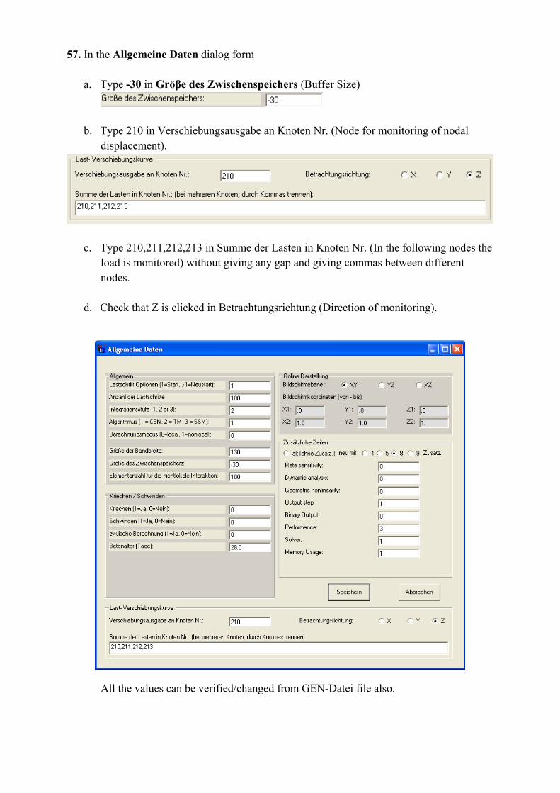
57. In the Allgemeine Daten dialog form a. Type -30 in Gröβe des Zwischenspeichers (Buffer Size)
b. Type 210 in Verschiebungsausgabe an Knoten Nr. (Node for monitoring of nodal displacement).
c. Type 210,211,212,213 in Summe der Lasten in Knoten Nr. (In the following nodes the load is monitored) without giving any gap and giving commas between different nodes.
d. Check that Z is clicked in Betrachtungsrichtung (Direction of monitoring).
All the values can be verified/changed from GEN-Datei file also.
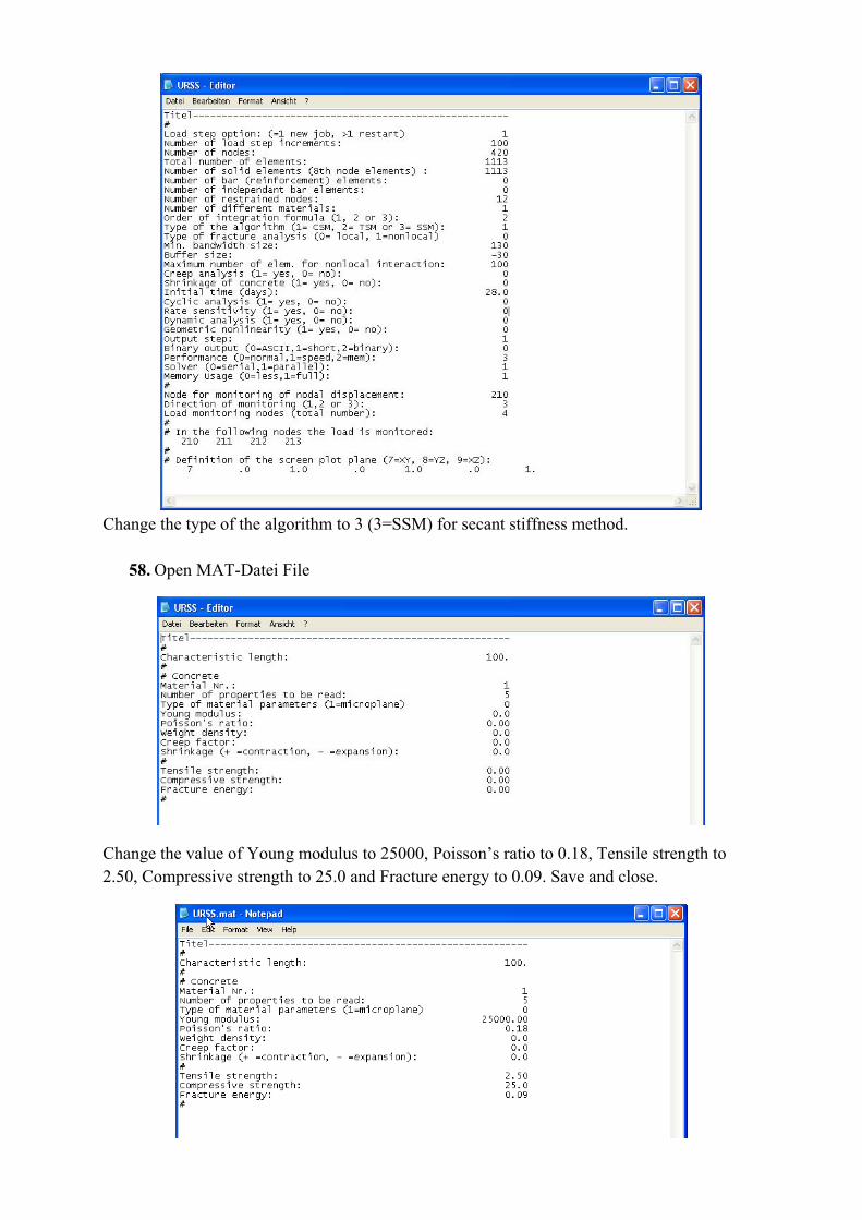
Change the type of the algorithm to 3 (3=SSM) for secant stiffness method.
58. Open MAT-Datei File
Change the value of Young modulus to 25000, Poisson’s ratio to 0.18, Tensile strength to 2.50, Compressive strength to 25.0 and Fracture energy to 0.09. Save and close.
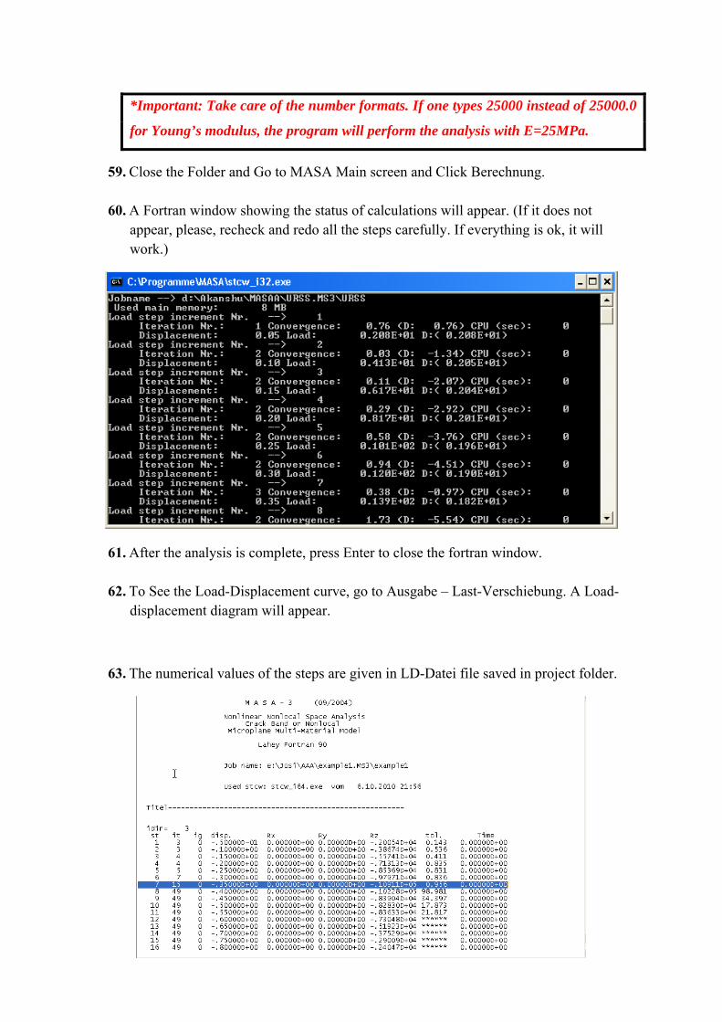
*Important: Take care of the number formats. If one types 25000 instead of 25000.0
for Young’s modulus, the program will perform the analysis with E=25MPa.
59. Close the Folder and Go to MASA Main screen and Click Berechnung.
60. A Fortran window showing the status of calculations will appear. (If it does not appear, please, recheck and redo all the steps carefully. If everything is ok, it will work.)
61. After the analysis is complete, press Enter to close the fortran window.
62. To See the Load-Displacement curve, go to Ausgabe – Last-Verschiebung. A Load-displacement diagram will appear.
63. The numerical values of the steps are given in LD-Datei file saved in project folder.
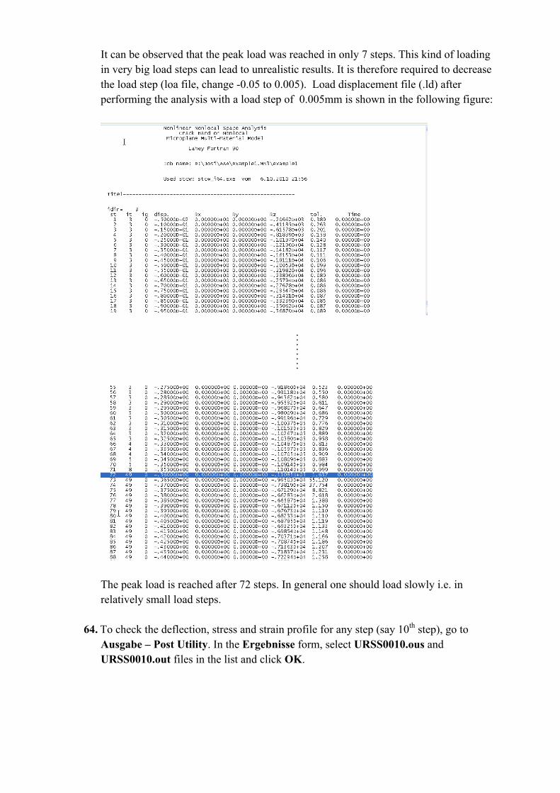
It can be observed that the peak load was reached in only 7 steps. This kind of loading in very big load steps can lead to unrealistic results. It is therefore required to decrease the load step (loa file, change -0.05 to 0.005). Load displacement file (.ld) after performing the analysis with a load step of 0.005mm is shown in the following figure:
. . . . . . . .
The peak load is reached after 72 steps. In general one should load slowly i.e. in relatively small load steps.
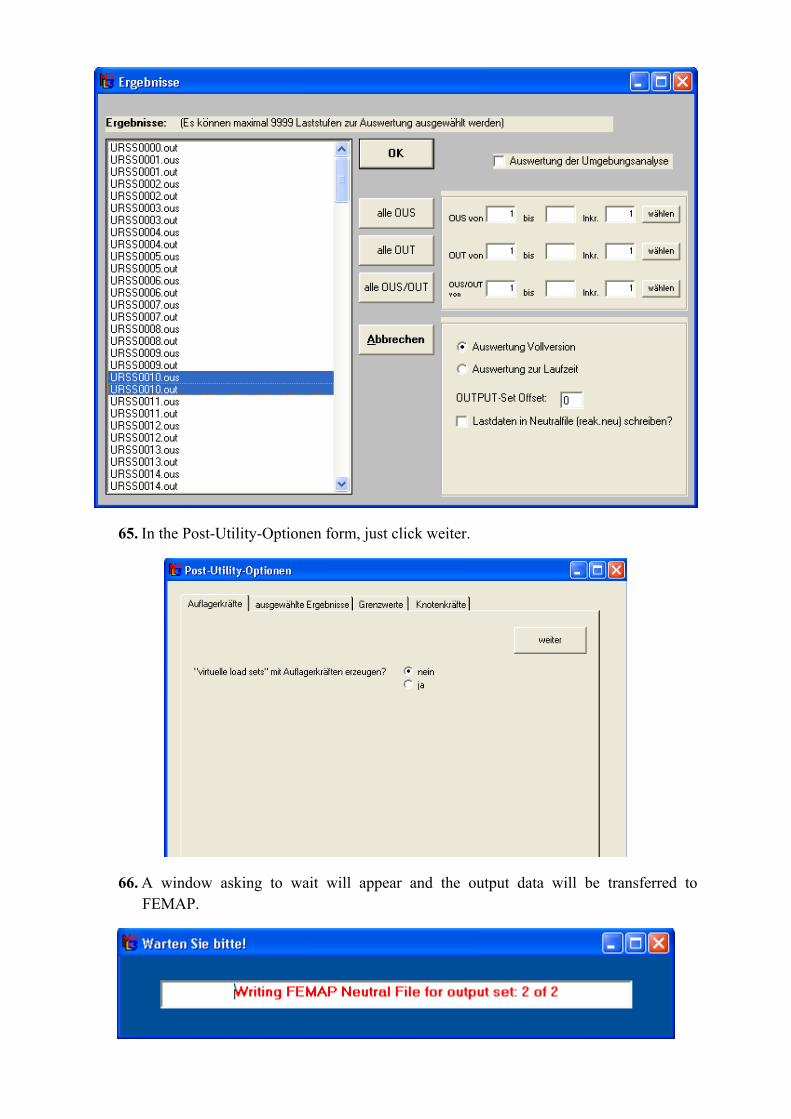
64. To check the deflection, stress and strain profile for any step (say 10th step), go to Ausgabe – Post Utility. In the Ergebnisse form, select URSS0010.ous and URSS0010.out files in the list and click OK.
65. In the Post-Utility-Optionen form, just click weiter.
66. A window asking to wait will appear and the output data will be transferred to FEMAP.
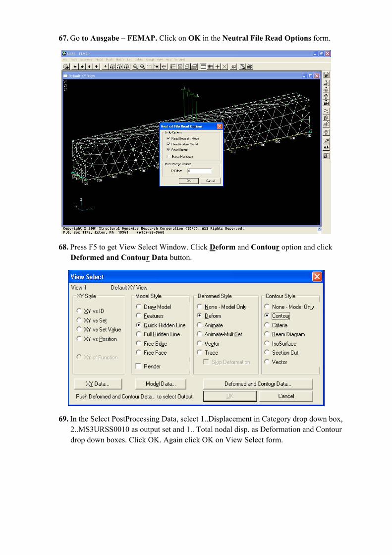
67. Go to Ausgabe – FEMAP. Click on OK in the Neutral File Read Options form.
68. Press F5 to get View Select Window. Click Deform and Contour option and click Deformed and Contour Data button.
69. In the Select PostProcessing Data, select 1..Displacement in Category drop down box, 2..MS3URSS0010 as output set and 1.. Total nodal disp. as Deformation and Contour drop down boxes. Click OK. Again click OK on View Select form.
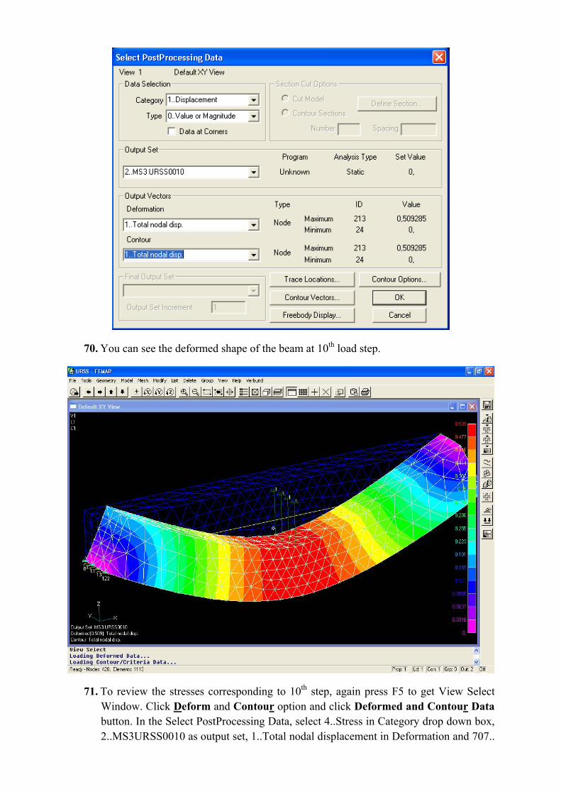
70. You can see the deformed shape of the beam at 10th load step.
71. To review the stresses corresponding to 10th step, again press F5 to get View Select Window. Click Deform and Contour option and click Deformed and Contour Data button. In the Select PostProcessing Data, select 4..Stress in Category drop down box, 2..MS3URSS0010 as output set, 1..Total nodal displacement in Deformation and 707..
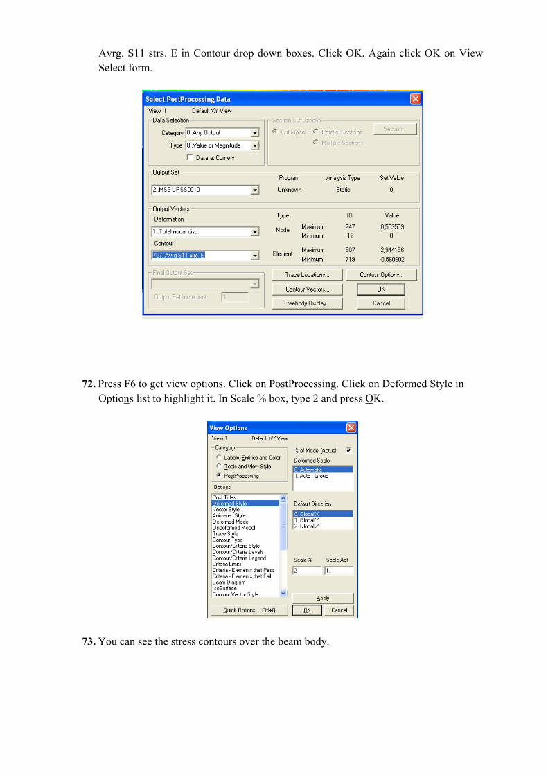
Avrg. S11 strs. E in Contour drop down boxes. Click OK. Again click OK on View Select form.
72. Press F6 to get view options. Click on PostProcessing. Click on Deformed Style in Options list to highlight it. In Scale % box, type 2 and press OK.
73. You can see the stress contours over the beam body.
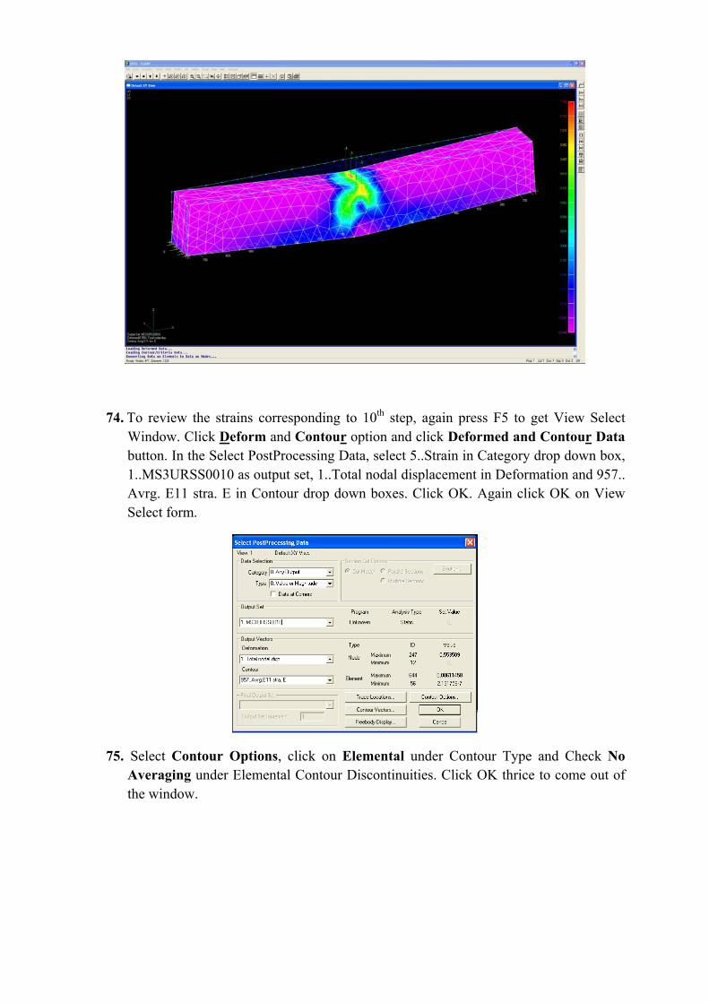
74. To review the strains corresponding to 10th step, again press F5 to get View Select Window. Click Deform and Contour option and click Deformed and Contour Data button. In the Select PostProcessing Data, select 5..Strain in Category drop down box, 1..MS3URSS0010 as output set, 1..Total nodal displacement in Deformation and 957.. Avrg. E11 stra. E in Contour drop down boxes. Click OK. Again click OK on View Select form.
75. Select Contour Options, click on Elemental under Contour Type and Check No Averaging under Elemental Contour Discontinuities. Click OK thrice to come out of the window.
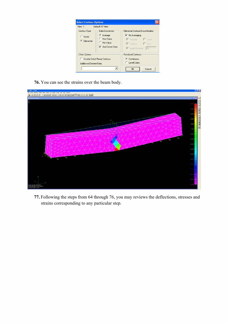
76. You can see the strains over the beam body.
77. Following the steps from 64 through 76, you may reviews the deflections, stresses and strains corresponding to any particular step.

TUTORIAL 2
ANALYSIS OF SINGLY REINFORCED SIMPLY SUPPORTED
RECTANGULAR RCC BEAM UNDER THREE POINT BENDING
(Input files available under name :example2.ms3)
In this tutorial, you will learn
1. Working with more than one solids
2. Working with more than one materials
3. Modeling of Reinforcement
4. Modeling of real life support conditions
5. Working with Hex meshing
6. Changing properties of elements
7. Visualizing progress of strains etc with each step
The details for the beam are given below.
Compressive strength of concrete = 25 MPa
Tensile strength of concrete = 2.5 MPa
Elastic Modulus of concrete = 25000 MPa
Elastic Modulus of Reinforcement and Steel Supports = 200000 MPa
Poisson’s Ratio for Concrete = 0.18
Reinforcement area = 2 bars of 50 mm2 each
Reinforcement yield stress = 480.0
Reinforcement hardening modulus = 2000.0
Reinforcement ultimate stress = 580.0
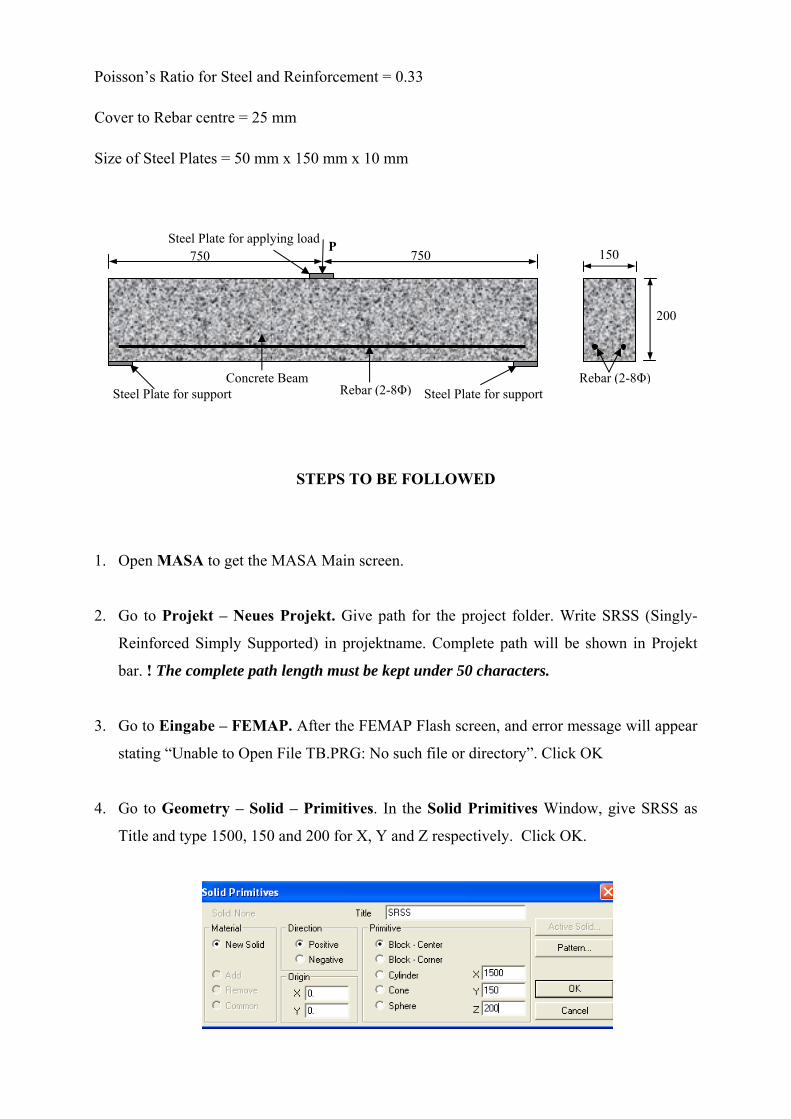
Poisson’s Ratio for Steel and Reinforcement = 0.33
Cover to Rebar centre = 25 mm
Size of Steel Plates = 50 mm x 150 mm x 10 mm
STEPS TO BE FOLLOWED
1. Open MASA to get the MASA Main screen.
2. Go to Projekt – Neues Projekt. Give path for the project folder. Write SRSS (Singly-
Reinforced Simply Supported) in projektname. Complete path will be shown in Projekt
bar. ! The complete path length must be kept under 50 characters.
3. Go to Eingabe – FEMAP. After the FEMAP Flash screen, and error message will appear
stating “Unable to Open File TB.PRG: No such file or directory”. Click OK
4. Go to Geometry – Solid – Primitives. In the Solid Primitives Window, give SRSS as
Title and type 1500, 150 and 200 for X, Y and Z respectively. Click OK.
750 750 P
150
200
Concrete Beam Rebar (2-8Φ)Steel Plate for support Steel Plate for support
Steel Plate for applying load
Rebar (2-8Φ)
5. Window showing the beam in Default XY View will appear. Click on Dyn Rotate
button to rotate the model and obtain desirable view. (It is advised to keep Z axis as
vertical upwards).
6. Press Ctrl + Q to get View Quick Options dialog box. Under the Geometry column,
uncheck the Surface and Volume Check boxes. Click Done. Now we will be able to see
only boundary lines of the beam.
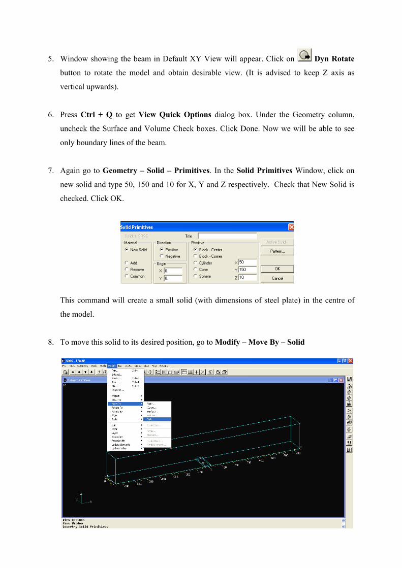
7. Again go to Geometry – Solid – Primitives. In the Solid Primitives Window, click on
new solid and type 50, 150 and 10 for X, Y and Z respectively. Check that New Solid is
checked. Click OK.
This command will create a small solid (with dimensions of steel plate) in the centre of
the model.
8. To move this solid to its desired position, go to Modify – Move By – Solid
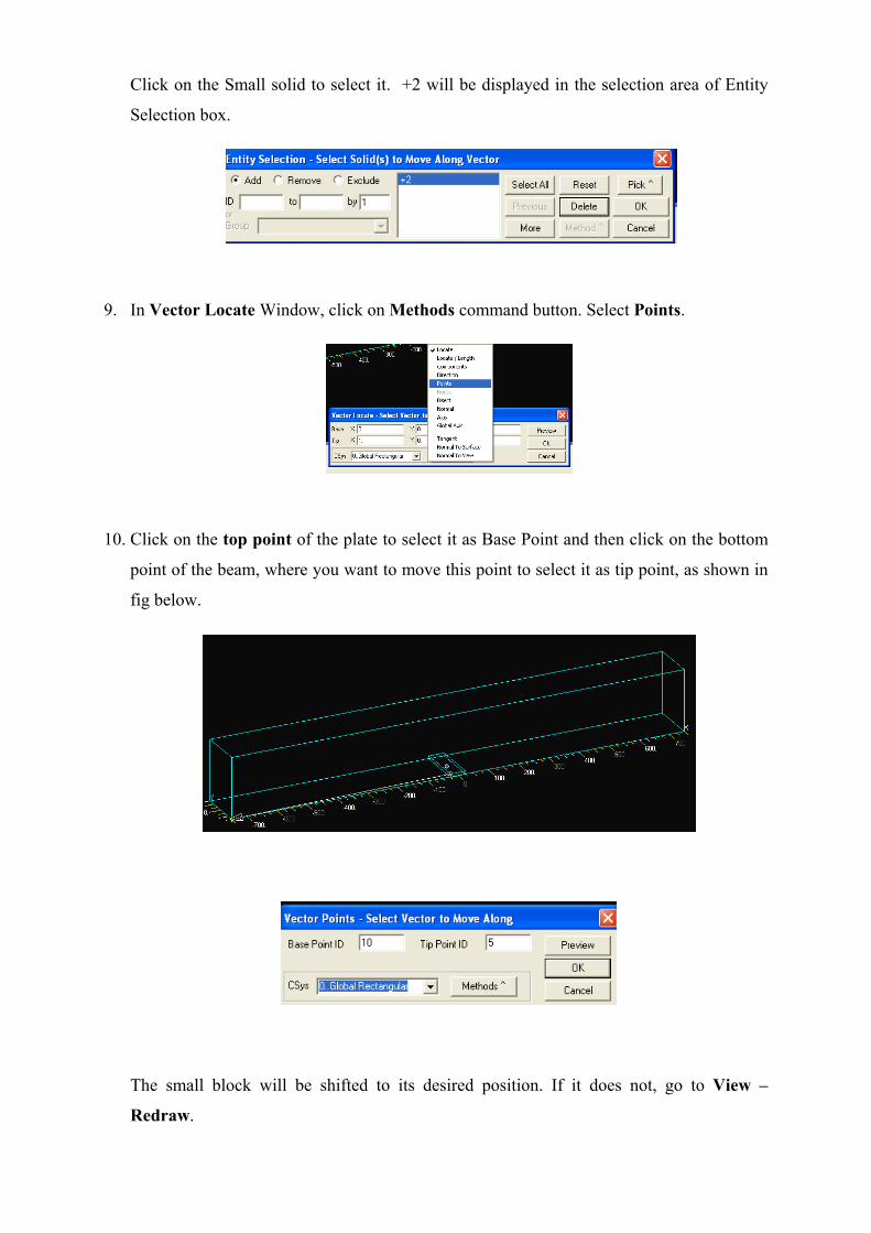
Click on the Small solid to select it. +2 will be displayed in the selection area of Entity
Selection box.
9. In Vector Locate Window, click on Methods command button. Select Points.
10. Click on the top point of the plate to select it as Base Point and then click on the bottom
point of the beam, where you want to move this point to select it as tip point, as shown in
fig below.
The small block will be shifted to its desired position. If it does not, go to View –
Redraw.
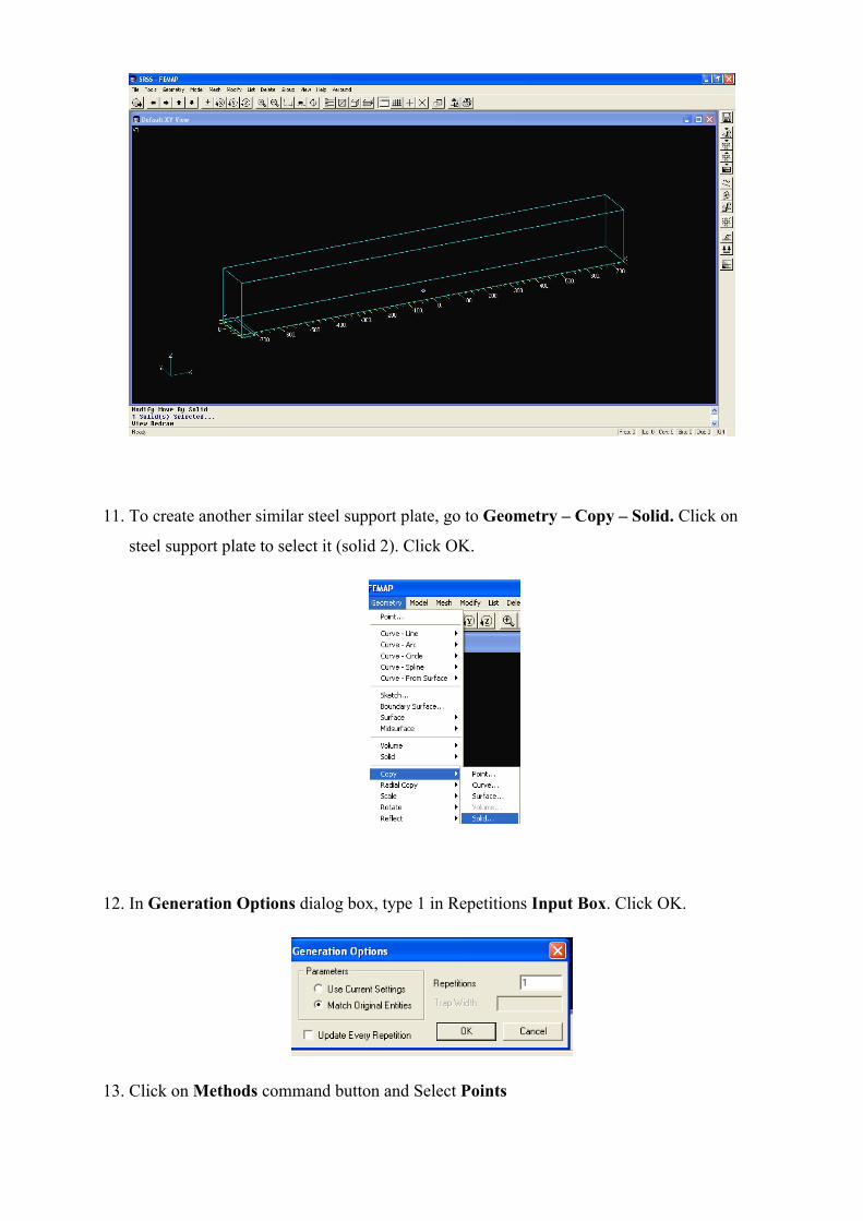
11. To create another similar steel support plate, go to Geometry – Copy – Solid. Click on
steel support plate to select it (solid 2). Click OK.
12. In Generation Options dialog box, type 1 in Repetitions Input Box. Click OK.
13. Click on Methods command button and Select Points
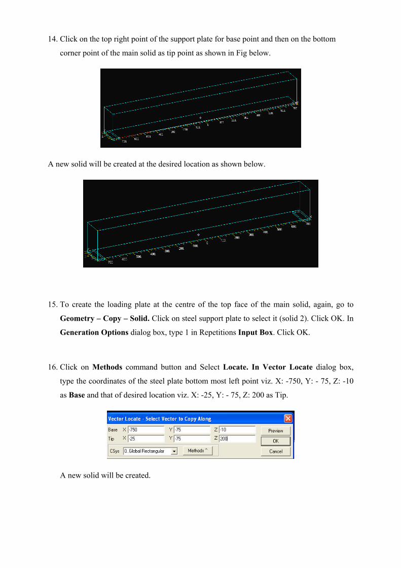
14. Click on the top right point of the support plate for base point and then on the bottom
corner point of the main solid as tip point as shown in Fig below.
A new solid will be created at the desired location as shown below.
15. To create the loading plate at the centre of the top face of the main solid, again, go to
Geometry – Copy – Solid. Click on steel support plate to select it (solid 2). Click OK. In
Generation Options dialog box, type 1 in Repetitions Input Box. Click OK.
16. Click on Methods command button and Select Locate. In Vector Locate dialog box,
type the coordinates of the steel plate bottom most left point viz. X: -750, Y: - 75, Z: -10
as Base and that of desired location viz. X: -25, Y: - 75, Z: 200 as Tip.
A new solid will be created.

17. Go to Geometry – Point. In the Locate dialog box, type -750, 50 and 25 for X, Y and Z
respectively as shown below.
Repeat for
X = -750; Y = 50; Z = 25
X = 750; Y = 50; Z = 25
X = 750; Y = -50; Z = 25
Four points, as shown below, will be created
18. Go to Geometry – Curve-Line – Points…
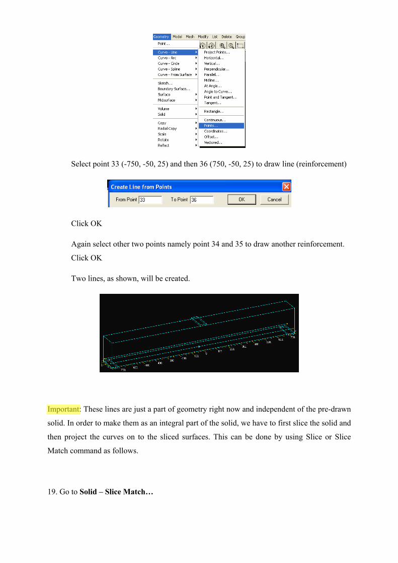
Select point 33 (-750, -50, 25) and then 36 (750, -50, 25) to draw line (reinforcement)
Click OK
Again select other two points namely point 34 and 35 to draw another reinforcement.
Click OK
Two lines, as shown, will be created.
Important: These lines are just a part of geometry right now and independent of the pre-drawn
solid. In order to make them as an integral part of the solid, we have to first slice the solid and
then project the curves on to the sliced surfaces. This can be done by using Slice or Slice
Match command as follows.
19. Go to Solid – Slice Match…
natalija.bede
Highlight
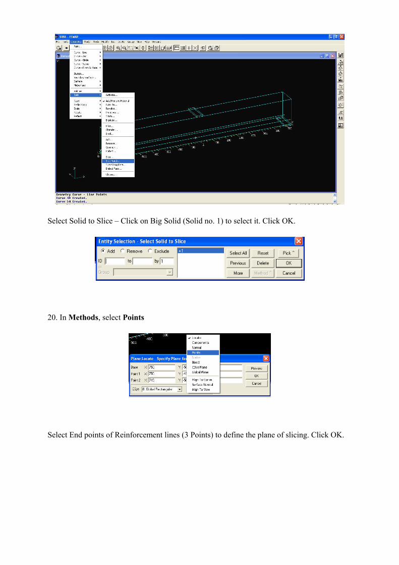
Select Solid to Slice – Click on Big Solid (Solid no. 1) to select it. Click OK.
20. In Methods, select Points
Select End points of Reinforcement lines (3 Points) to define the plane of slicing. Click OK.
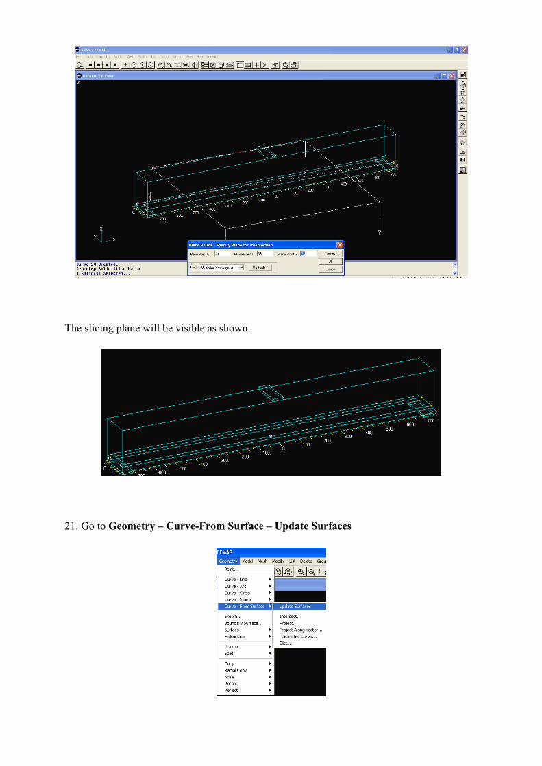
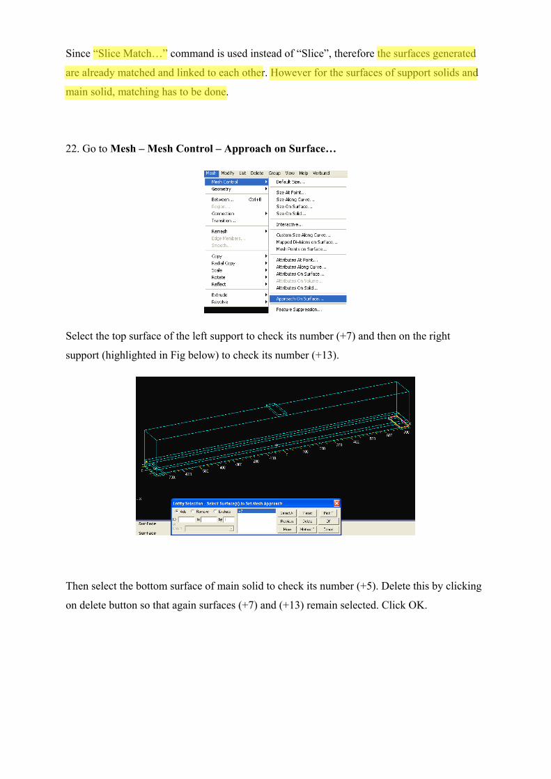
The slicing plane will be visible as shown.
21. Go to Geometry – Curve-From Surface – Update Surfaces
Since “Slice Match…” command is used instead of “Slice”, therefore the surfaces generated
are already matched and linked to each other. However for the surfaces of support solids and
main solid, matching has to be done.
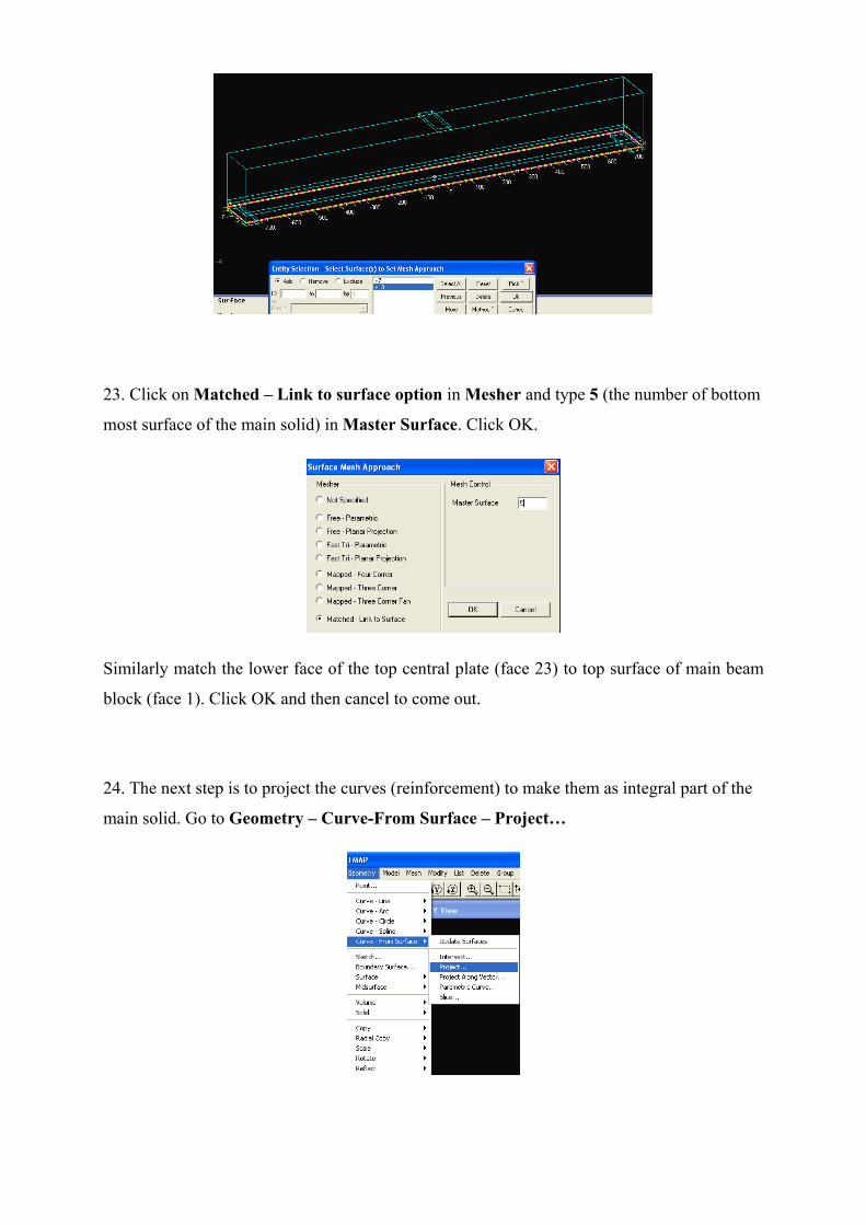
22. Go to Mesh – Mesh Control – Approach on Surface…
Select the top surface of the left support to check its number (+7) and then on the right
support (highlighted in Fig below) to check its number (+13).
Then select the bottom surface of main solid to check its number (+5). Delete this by clicking
on delete button so that again surfaces (+7) and (+13) remain selected. Click OK.
natalija.bede
Highlight
natalija.bede
Highlight
natalija.bede
Highlight
23. Click on Matched – Link to surface option in Mesher and type 5 (the number of bottom
most surface of the main solid) in Master Surface. Click OK.
Similarly match the lower face of the top central plate (face 23) to top surface of main beam
block (face 1). Click OK and then cancel to come out.
24. The next step is to project the curves (reinforcement) to make them as integral part of the
main solid. Go to Geometry – Curve-From Surface – Project…
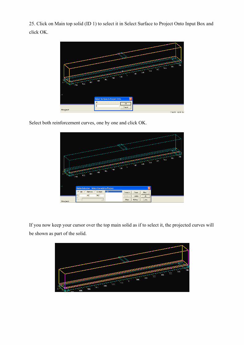
25. Click on Main top solid (ID 1) to select it in Select Surface to Project Onto Input Box and
click OK.
Select both reinforcement curves, one by one and click OK.
If you now keep your cursor over the top main solid as if to select it, the projected curves will
be shown as part of the solid.
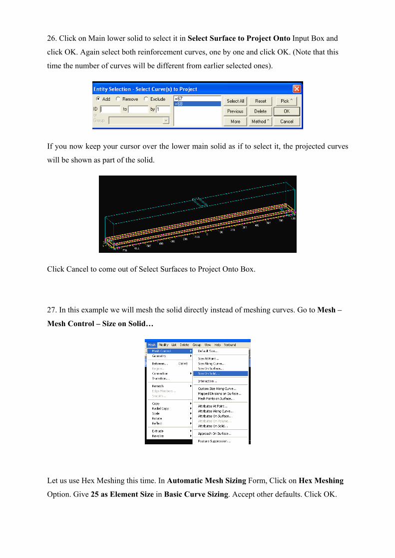
26. Click on Main lower solid to select it in Select Surface to Project Onto Input Box and
click OK. Again select both reinforcement curves, one by one and click OK. (Note that this
time the number of curves will be different from earlier selected ones).
If you now keep your cursor over the lower main solid as if to select it, the projected curves
will be shown as part of the solid.
Click Cancel to come out of Select Surfaces to Project Onto Box.
27. In this example we will mesh the solid directly instead of meshing curves. Go to Mesh –
Mesh Control – Size on Solid…
Let us use Hex Meshing this time. In Automatic Mesh Sizing Form, Click on Hex Meshing
Option. Give 25 as Element Size in Basic Curve Sizing. Accept other defaults. Click OK.
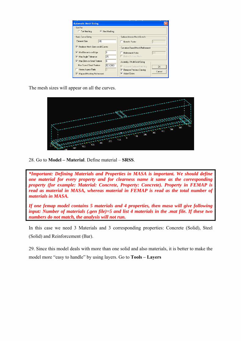
The mesh sizes will appear on all the curves.
28. Go to Model – Material. Define material – SRSS.
*Important: Defining Materials and Properties in MASA is important. We should define one material for every property and for clearness name it same as the corresponding property (for example: Material: Concrete, Property: Concrete). Property in FEMAP is read as material in MASA, whereas material in FEMAP is read as the total number of materials in MASA.
If one femap model contains 5 materials and 4 properties, then masa will give following input: Number of materials (.gen file)=5 and list 4 materials in the .mat file. If these two numbers do not match, the analysis will not run.
In this case we need 3 Materials and 3 corresponding properties: Concrete (Solid), Steel
(Solid) and Reinforcement (Bar).
29. Since this model deals with more than one solid and also materials, it is better to make the
model more “easy to handle” by using layers. Go to Tools – Layers
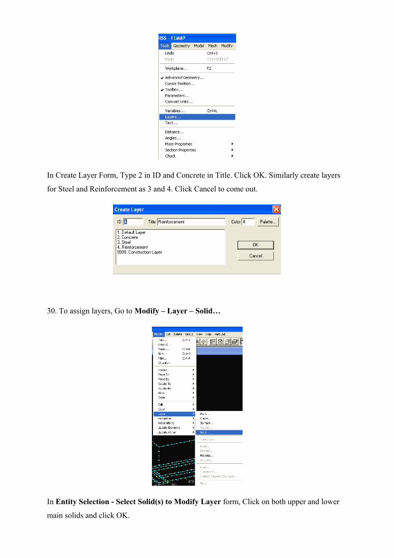
In Create Layer Form, Type 2 in ID and Concrete in Title. Click OK. Similarly create layers
for Steel and Reinforcement as 3 and 4. Click Cancel to come out.
30. To assign layers, Go to Modify – Layer – Solid…
In Entity Selection - Select Solid(s) to Modify Layer form, Click on both upper and lower
main solids and click OK.
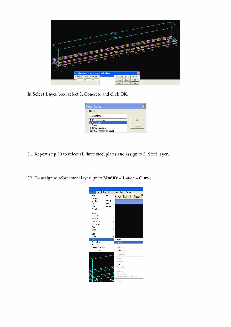
In Select Layer box, select 2..Concrete and click OK.
31. Repeat step 30 to select all three steel plates and assign to 3..Steel layer.
32. To assign reinforcement layer, go to Modify – Layer – Curve…
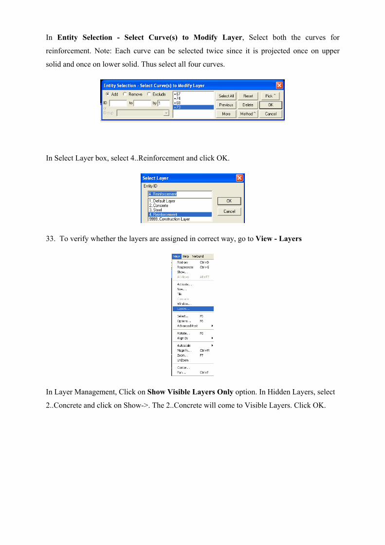
In Entity Selection - Select Curve(s) to Modify Layer, Select both the curves for
reinforcement. Note: Each curve can be selected twice since it is projected once on upper
solid and once on lower solid. Thus select all four curves.
In Select Layer box, select 4..Reinforcement and click OK.
33. To verify whether the layers are assigned in correct way, go to View - Layers
In Layer Management, Click on Show Visible Layers Only option. In Hidden Layers, select
2..Concrete and click on Show->. The 2..Concrete will come to Visible Layers. Click OK.
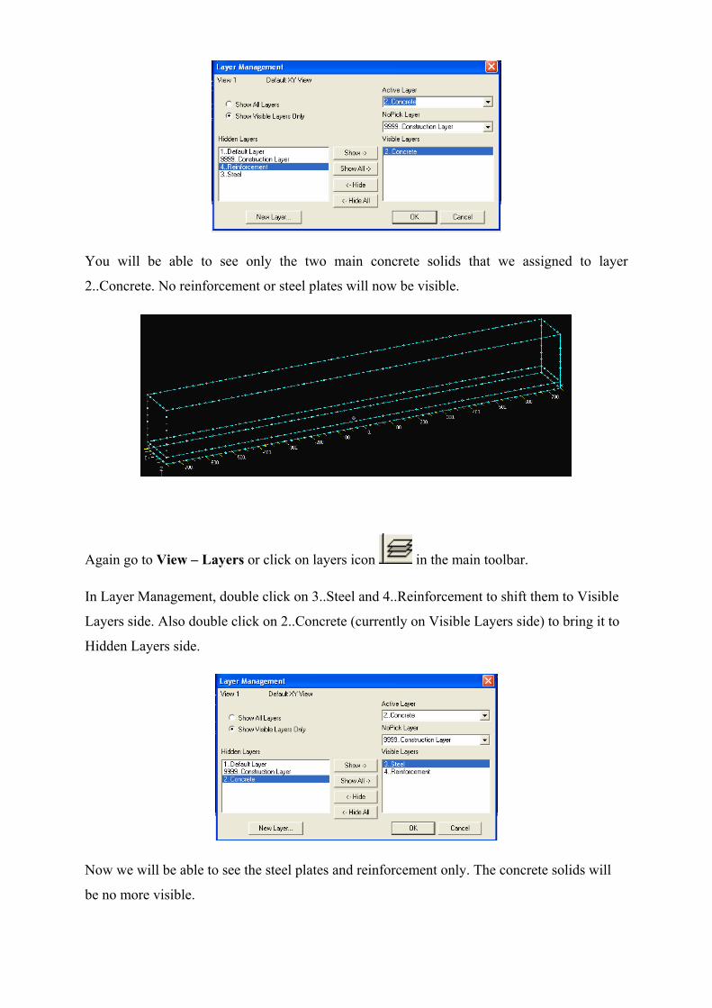
You will be able to see only the two main concrete solids that we assigned to layer
2..Concrete. No reinforcement or steel plates will now be visible.
Again go to View – Layers or click on layers icon in the main toolbar.
In Layer Management, double click on 3..Steel and 4..Reinforcement to shift them to Visible
Layers side. Also double click on 2..Concrete (currently on Visible Layers side) to bring it to
Hidden Layers side.
Now we will be able to see the steel plates and reinforcement only. The concrete solids will
be no more visible.
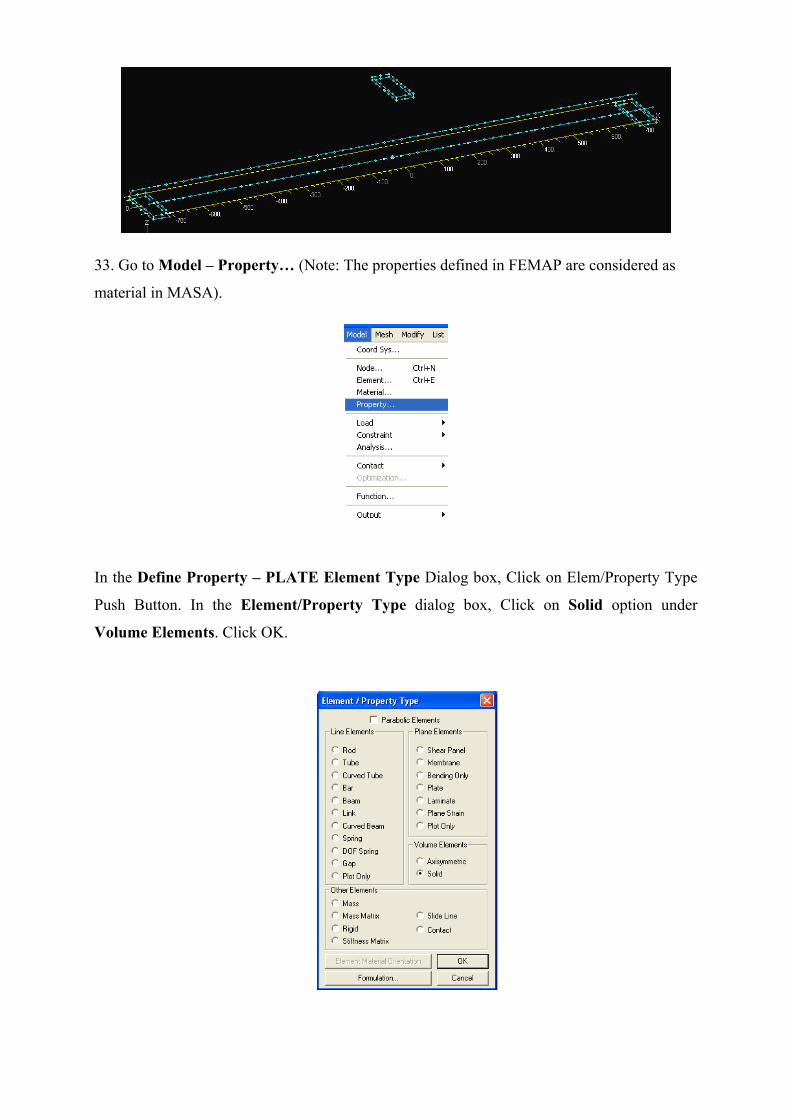
33. Go to Model – Property… (Note: The properties defined in FEMAP are considered as
material in MASA).
In the Define Property – PLATE Element Type Dialog box, Click on Elem/Property Type
Push Button. In the Element/Property Type dialog box, Click on Solid option under
Volume Elements. Click OK.
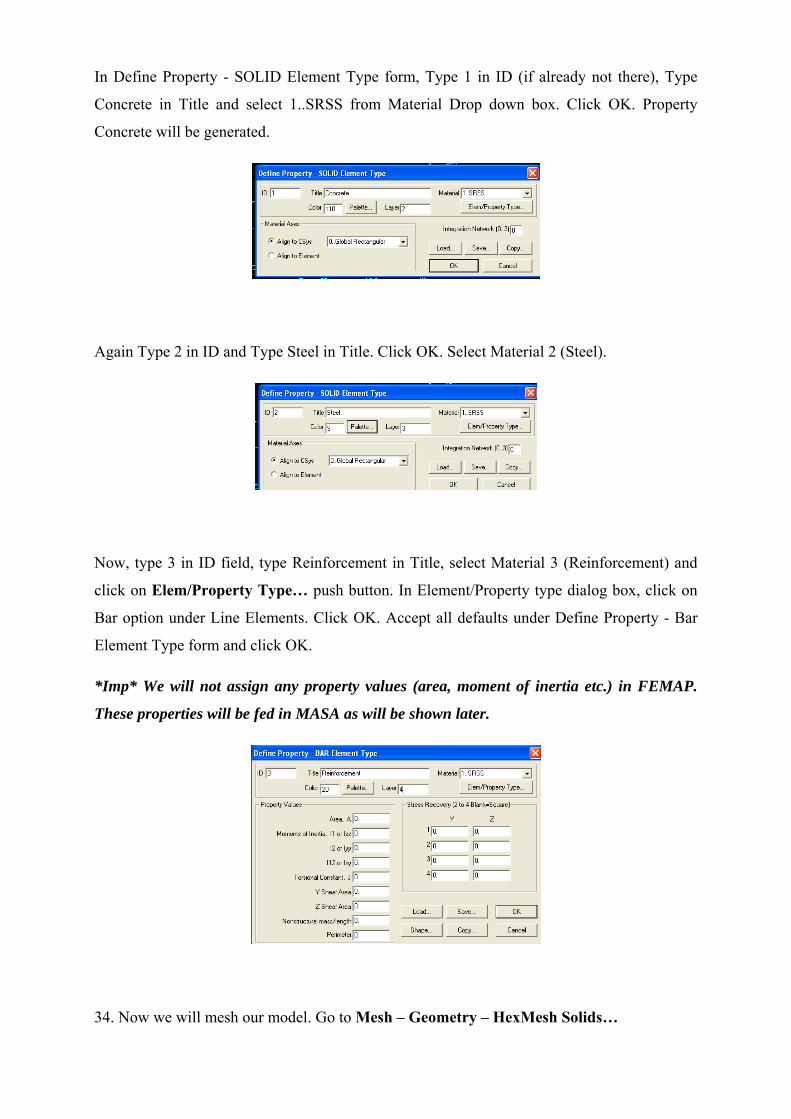
In Define Property - SOLID Element Type form, Type 1 in ID (if already not there), Type
Concrete in Title and select 1..SRSS from Material Drop down box. Click OK. Property
Concrete will be generated.
Again Type 2 in ID and Type Steel in Title. Click OK. Select Material 2 (Steel).
Now, type 3 in ID field, type Reinforcement in Title, select Material 3 (Reinforcement) and
click on Elem/Property Type… push button. In Element/Property type dialog box, click on
Bar option under Line Elements. Click OK. Accept all defaults under Define Property - Bar
Element Type form and click OK.
*Imp* We will not assign any property values (area, moment of inertia etc.) in FEMAP.
These properties will be fed in MASA as will be shown later.
34. Now we will mesh our model. Go to Mesh – Geometry – HexMesh Solids…
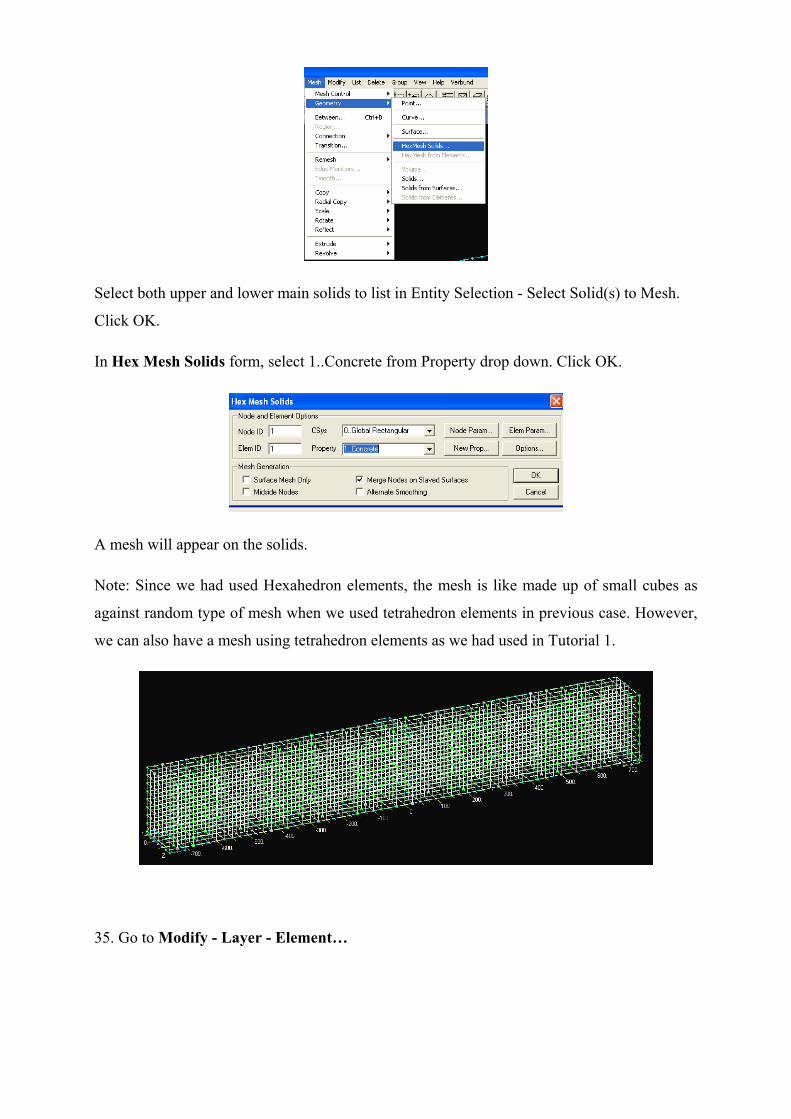
Select both upper and lower main solids to list in Entity Selection - Select Solid(s) to Mesh.
Click OK.
In Hex Mesh Solids form, select 1..Concrete from Property drop down. Click OK.
A mesh will appear on the solids.
Note: Since we had used Hexahedron elements, the mesh is like made up of small cubes as
against random type of mesh when we used tetrahedron elements in previous case. However,
we can also have a mesh using tetrahedron elements as we had used in Tutorial 1.
35. Go to Modify - Layer - Element…
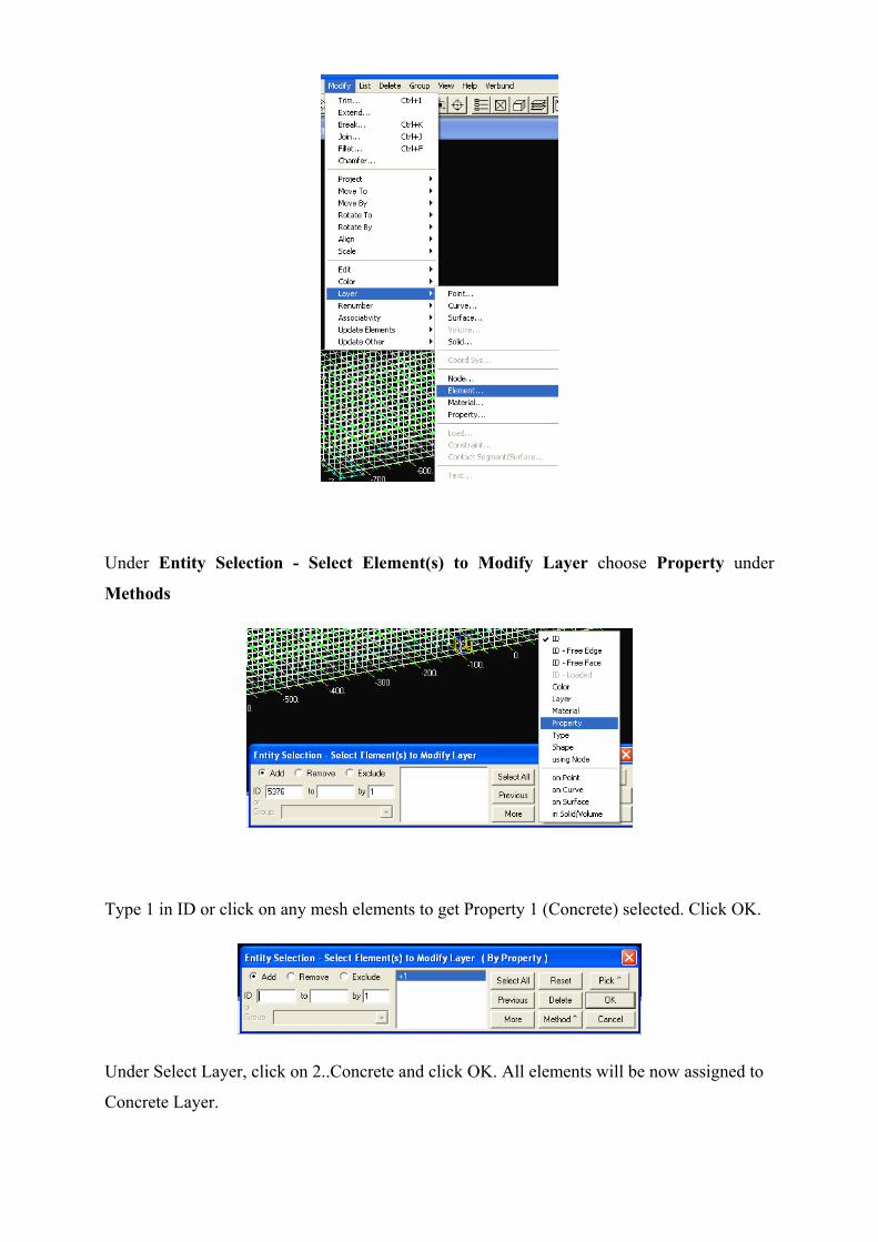
Under Entity Selection - Select Element(s) to Modify Layer choose Property under
Methods
Type 1 in ID or click on any mesh elements to get Property 1 (Concrete) selected. Click OK.
Under Select Layer, click on 2..Concrete and click OK. All elements will be now assigned to
Concrete Layer.
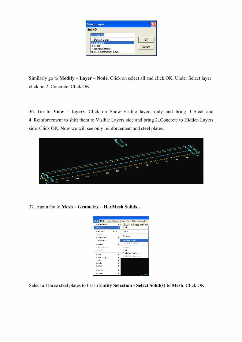
Similarly go to Modify – Layer – Node. Click on select all and click OK. Under Select layer
click on 2..Concrete. Click OK.
36. Go to View – layers. Click on Show visible layers only and bring 3..Steel and
4..Reinforcement to shift them to Visible Layers side and bring 2..Concrete to Hidden Layers
side. Click OK. Now we will see only reinforcement and steel plates.
37. Again Go to Mesh – Geometry – HexMesh Solids…
Select all three steel plates to list in Entity Selection - Select Solid(s) to Mesh. Click OK.
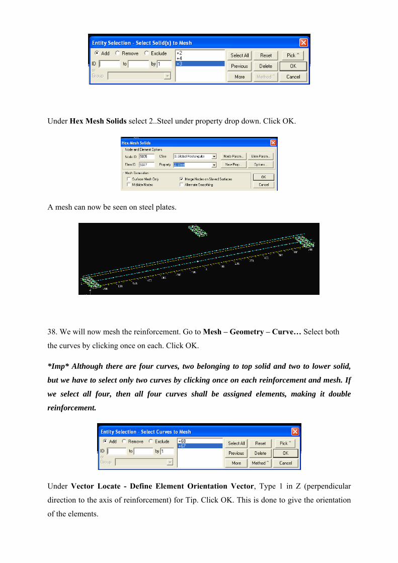
Under Hex Mesh Solids select 2..Steel under property drop down. Click OK.
A mesh can now be seen on steel plates.
38. We will now mesh the reinforcement. Go to Mesh – Geometry – Curve… Select both
the curves by clicking once on each. Click OK.
*Imp* Although there are four curves, two belonging to top solid and two to lower solid,
but we have to select only two curves by clicking once on each reinforcement and mesh. If
we select all four, then all four curves shall be assigned elements, making it double
reinforcement.
Under Vector Locate - Define Element Orientation Vector, Type 1 in Z (perpendicular
direction to the axis of reinforcement) for Tip. Click OK. This is done to give the orientation
of the elements.
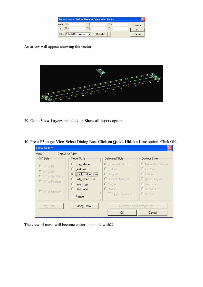
An arrow will appear showing the vector.
39. Go to View Layers and click on Show all layers option.
40. Press F5 to get View Select Dialog Box. Click on Quick Hidden Line option. Click OK.
The view of mesh will become easier to handle with.
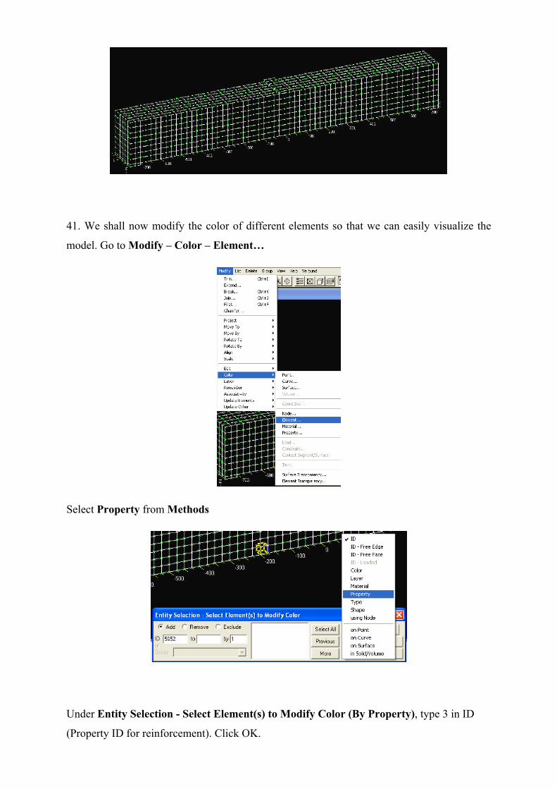
41. We shall now modify the color of different elements so that we can easily visualize the
model. Go to Modify – Color – Element…
Select Property from Methods
Under Entity Selection - Select Element(s) to Modify Color (By Property), type 3 in ID
(Property ID for reinforcement). Click OK.
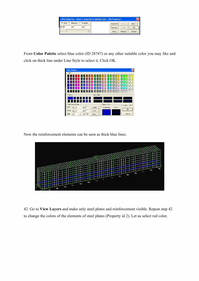
From Color Palette select blue color (ID 28747) or any other suitable color you may like and
click on thick line under Line Style to select it. Click OK.
Now the reinforcement elements can be seen as thick blue lines.
42. Go to View Layers and make only steel plates and reinforcement visible. Repeat step 42
to change the colors of the elements of steel plates (Property id 2). Let us select red color.
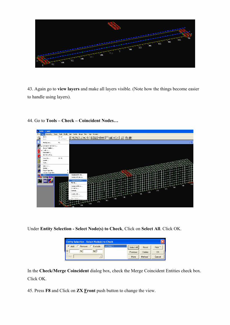
43. Again go to view layers and make all layers visible. (Note how the things become easier
to handle using layers).
44. Go to Tools – Check – Coincident Nodes…
Under Entity Selection - Select Node(s) to Check, Click on Select All. Click OK.
In the Check/Merge Coincident dialog box, check the Merge Coincident Entities check box.
Click OK.
45. Press F8 and Click on ZX Front push button to change the view.
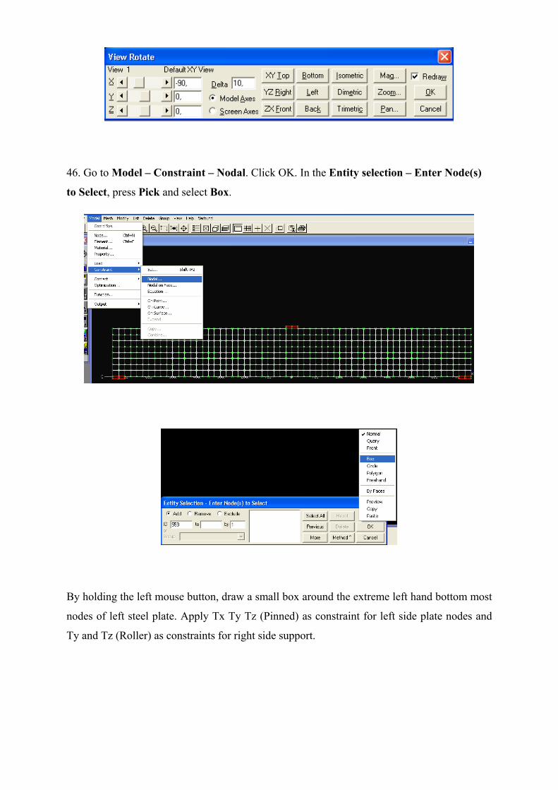
46. Go to Model – Constraint – Nodal. Click OK. In the Entity selection – Enter Node(s)
to Select, press Pick and select Box.
By holding the left mouse button, draw a small box around the extreme left hand bottom most
nodes of left steel plate. Apply Tx Ty Tz (Pinned) as constraint for left side plate nodes and
Ty and Tz (Roller) as constraints for right side support.
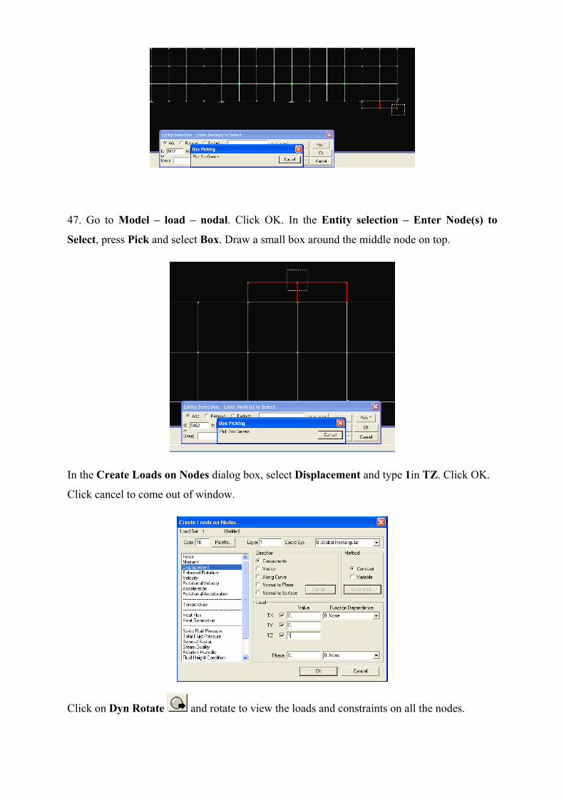
47. Go to Model – load – nodal. Click OK. In the Entity selection – Enter Node(s) to
Select, press Pick and select Box. Draw a small box around the middle node on top.
In the Create Loads on Nodes dialog box, select Displacement and type 1in TZ. Click OK.
Click cancel to come out of window.
Click on Dyn Rotate and rotate to view the loads and constraints on all the nodes.
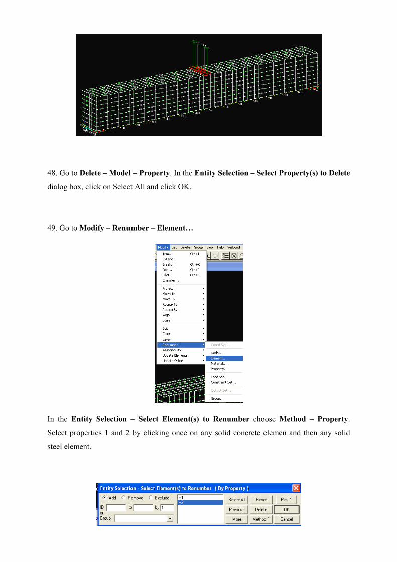
48. Go to Delete – Model – Property. In the Entity Selection – Select Property(s) to Delete
dialog box, click on Select All and click OK.
49. Go to Modify – Renumber – Element…
In the Entity Selection – Select Element(s) to Renumber choose Method – Property.
Select properties 1 and 2 by clicking once on any solid concrete elemen and then any solid
steel element.
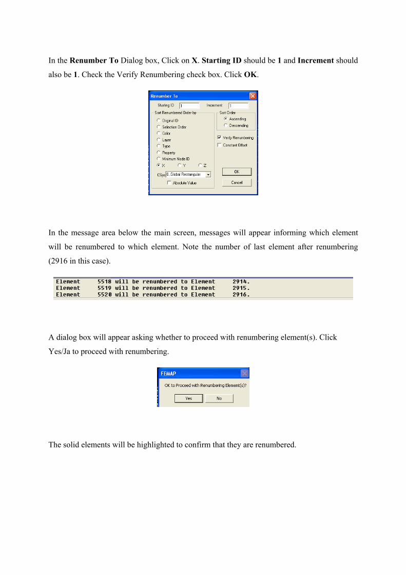
In the Renumber To Dialog box, Click on X. Starting ID should be 1 and Increment should
also be 1. Check the Verify Renumbering check box. Click OK.
In the message area below the main screen, messages will appear informing which element
will be renumbered to which element. Note the number of last element after renumbering
(2916 in this case).
A dialog box will appear asking whether to proceed with renumbering element(s). Click
Yes/Ja to proceed with renumbering.
The solid elements will be highlighted to confirm that they are renumbered.
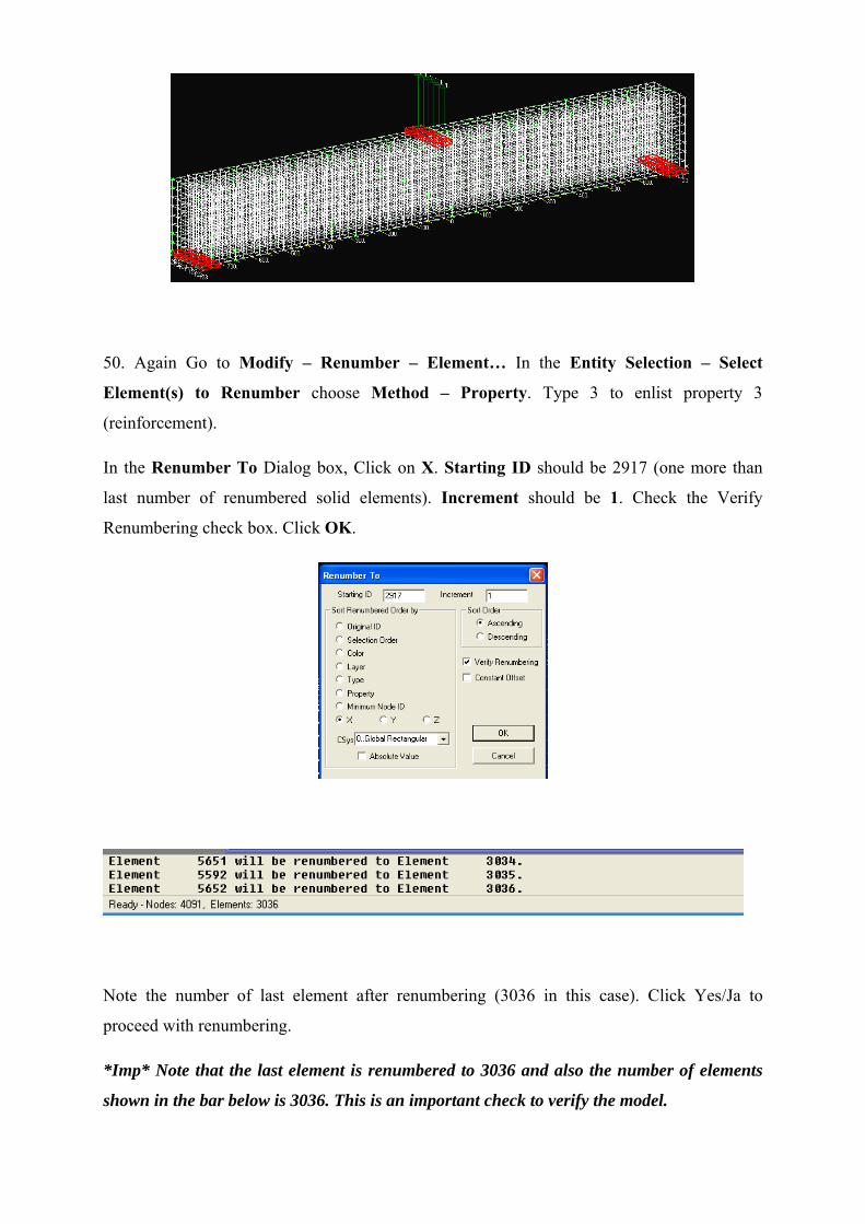
50. Again Go to Modify – Renumber – Element… In the Entity Selection – Select
Element(s) to Renumber choose Method – Property. Type 3 to enlist property 3
(reinforcement).
In the Renumber To Dialog box, Click on X. Starting ID should be 2917 (one more than
last number of renumbered solid elements). Increment should be 1. Check the Verify
Renumbering check box. Click OK.
Note the number of last element after renumbering (3036 in this case). Click Yes/Ja to
proceed with renumbering.
*Imp* Note that the last element is renumbered to 3036 and also the number of elements
shown in the bar below is 3036. This is an important check to verify the model.
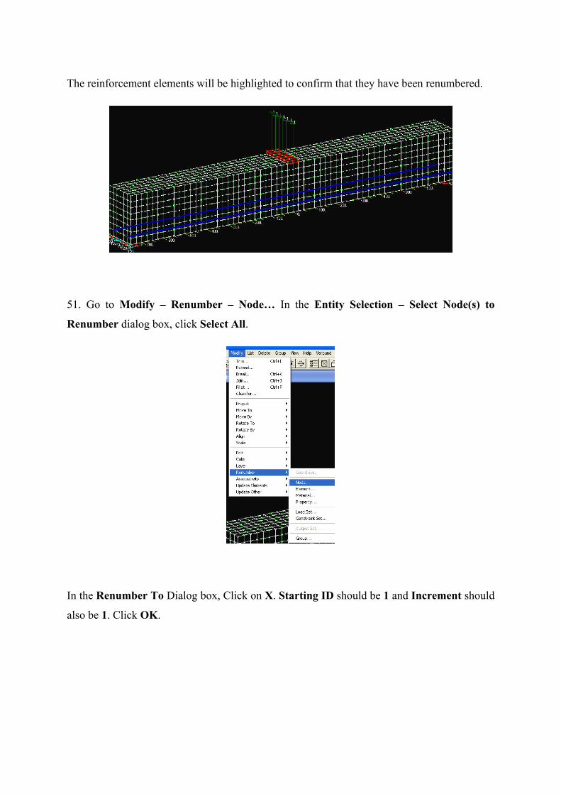
The reinforcement elements will be highlighted to confirm that they have been renumbered.
51. Go to Modify – Renumber – Node… In the Entity Selection – Select Node(s) to
Renumber dialog box, click Select All.
In the Renumber To Dialog box, Click on X. Starting ID should be 1 and Increment should
also be 1. Click OK.
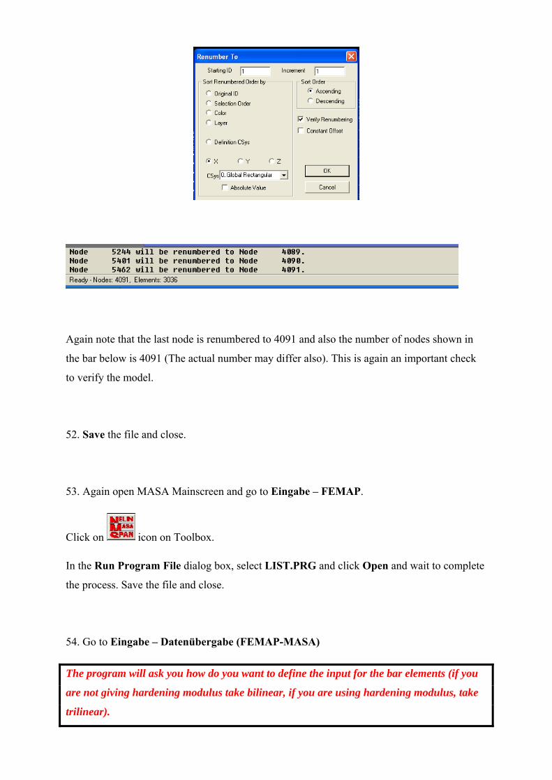
Again note that the last node is renumbered to 4091 and also the number of nodes shown in
the bar below is 4091 (The actual number may differ also). This is again an important check
to verify the model.
52. Save the file and close.
53. Again open MASA Mainscreen and go to Eingabe – FEMAP.
Click on icon on Toolbox.
In the Run Program File dialog box, select LIST.PRG and click Open and wait to complete
the process. Save the file and close.
54. Go to Eingabe – Datenübergabe (FEMAP-MASA)
The program will ask you how do you want to define the input for the bar elements (if you
are not giving hardening modulus take bilinear, if you are using hardening modulus, take
trilinear).
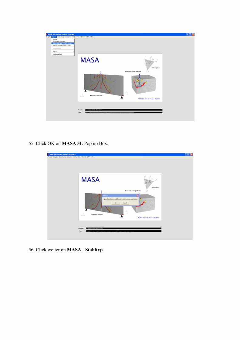
55. Click OK on MASA 3L Pop up Box.
56. Click weiter on MASA - Stahltyp

57. Go to folder SRSS.MS3 formed at the location whose path was given in Step 2.
58. Check the COR-Datei file to verify that the number of first node is 1 and that of the last
node is 4091 (Total number of nodes).
59. Check the ELE-Datei file to verify that the number of 1st element is 1 and that of last
element is 3036. Also note that the elements 2917 to 3036 are having only two node
connectivity showing that they are bar elements. Also we can see that for elements 2917 to
3036, the second row shows the material number as 3 (property id 3).
60. Open LOA-Datei File. This gives the load and constraint data. Notice the elements with a
value of 1 for third column of boundaries. This means that a load of 1 is assigned to these
nodes. Change Number of load increments to 100 and Displacement factor to – 0.1 (to apply
load in downward direction, in steps of 0.1 mm). Type 49 in Max. number of iterations. Save
and close.
61. Go to Gen-Datei file and check whether the Number of different materials is 3 (because
we have three properties in this case), Type of algorithm to 3 (SSM) and Buffer size to -30.
Type 3 for Performance, 0 for solver and 1 for Memory Usage.
62. Type the numbers of nodes in Summe der Lasten in Knoten Nr. (In the following nodes
the load is monitored) without giving any gap and giving commas between different nodes.
Type the number of node for monitoring nodal displacement in Verschiebungsausgabe an
Knoten Nr. Check that Z is clicked in Betrachtungsrichtung (Direction of monitoring).
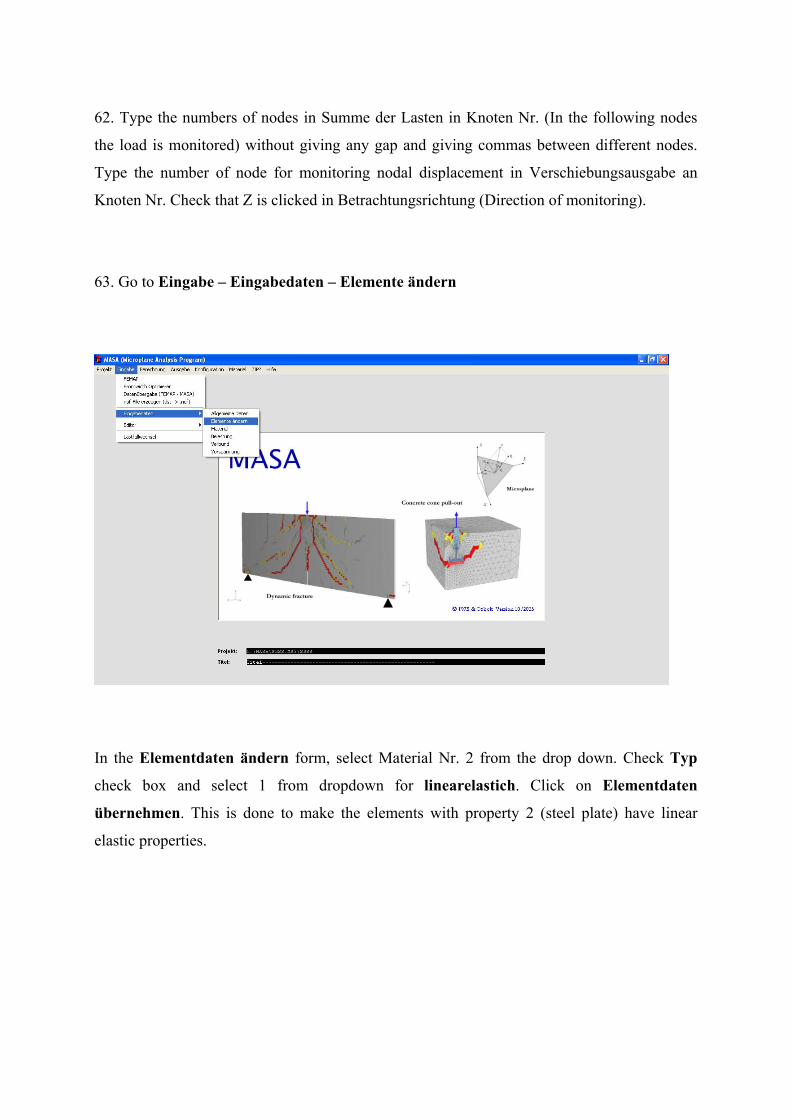
63. Go to Eingabe – Eingabedaten – Elemente ändern
In the Elementdaten ändern form, select Material Nr. 2 from the drop down. Check Typ
check box and select 1 from dropdown for linearelastich. Click on Elementdaten
übernehmen. This is done to make the elements with property 2 (steel plate) have linear
elastic properties.
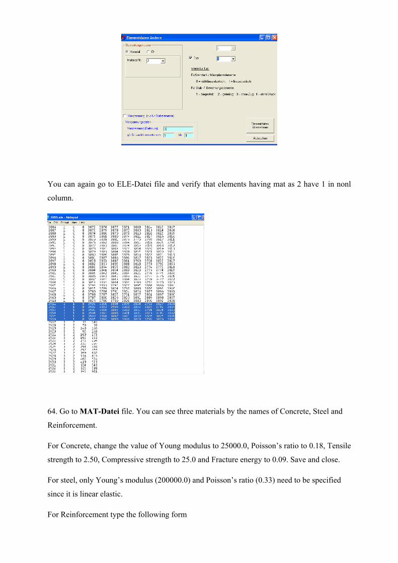
You can again go to ELE-Datei file and verify that elements having mat as 2 have 1 in nonl
column.
64. Go to MAT-Datei file. You can see three materials by the names of Concrete, Steel and
Reinforcement.
For Concrete, change the value of Young modulus to 25000.0, Poisson’s ratio to 0.18, Tensile
strength to 2.50, Compressive strength to 25.0 and Fracture energy to 0.09. Save and close.
For steel, only Young’s modulus (200000.0) and Poisson’s ratio (0.33) need to be specified
since it is linear elastic.
For Reinforcement type the following form
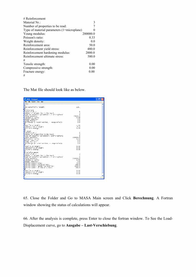
# Reinforcement Material Nr.: 3 Number of properties to be read: 7 Type of material parameters (1=microplane) 0 Young modulus: 200000.0 Poisson's ratio: 0.33 Weight density: 0.0 Reinforcement area: 50.0 Reinforcement yield stress: 480.0 Reinforcement hardening modulus: 2000.0 Reinforcement ultimate stress: 580.0 # Tensile strength: 0.00 Compressive strength: 0.00 Fracture energy: 0.00 #
The Mat file should look like as below.
65. Close the Folder and Go to MASA Main screen and Click Berechnung. A Fortran
window showing the status of calculations will appear.
66. After the analysis is complete, press Enter to close the fortran window. To See the Load-
Displacement curve, go to Ausgabe – Last-Verschiebung.
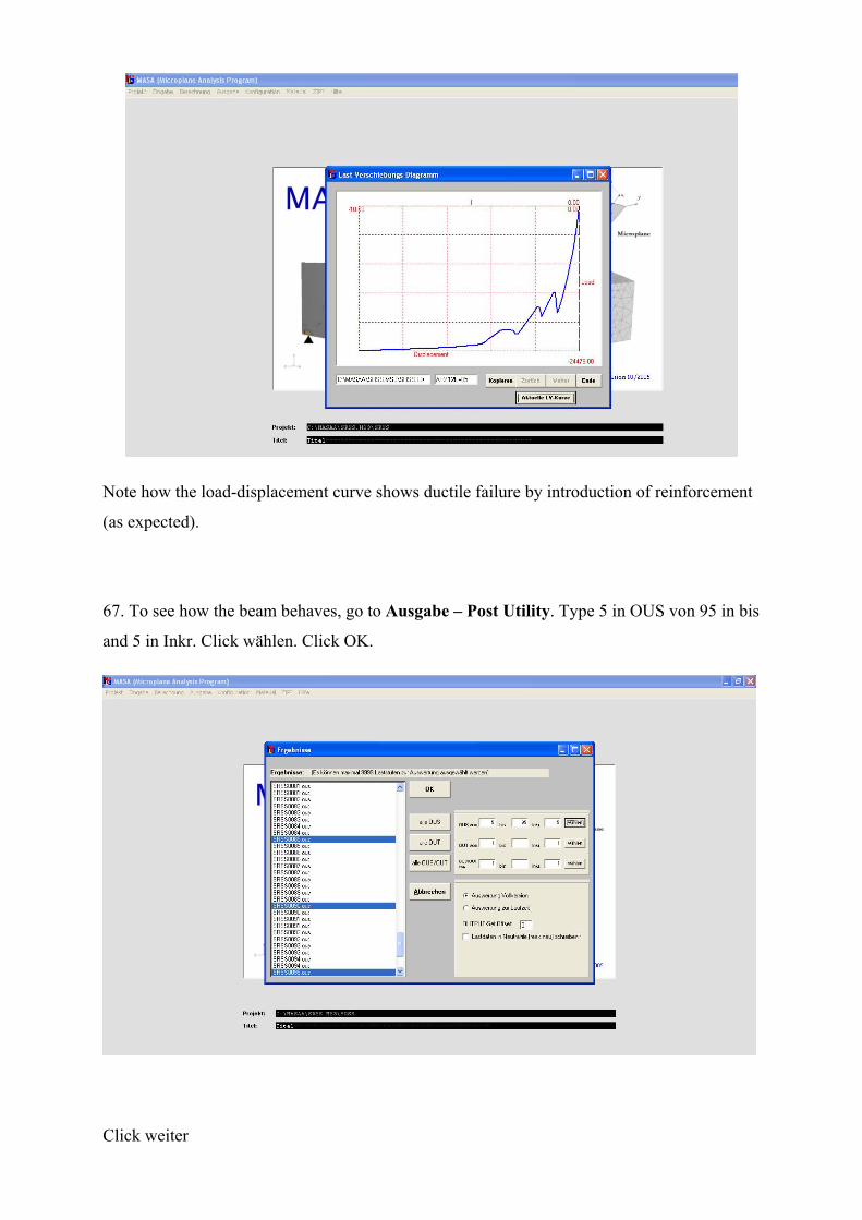
Note how the load-displacement curve shows ductile failure by introduction of reinforcement
(as expected).
67. To see how the beam behaves, go to Ausgabe – Post Utility. Type 5 in OUS von 95 in bis
and 5 in Inkr. Click wählen. Click OK.
Click weiter
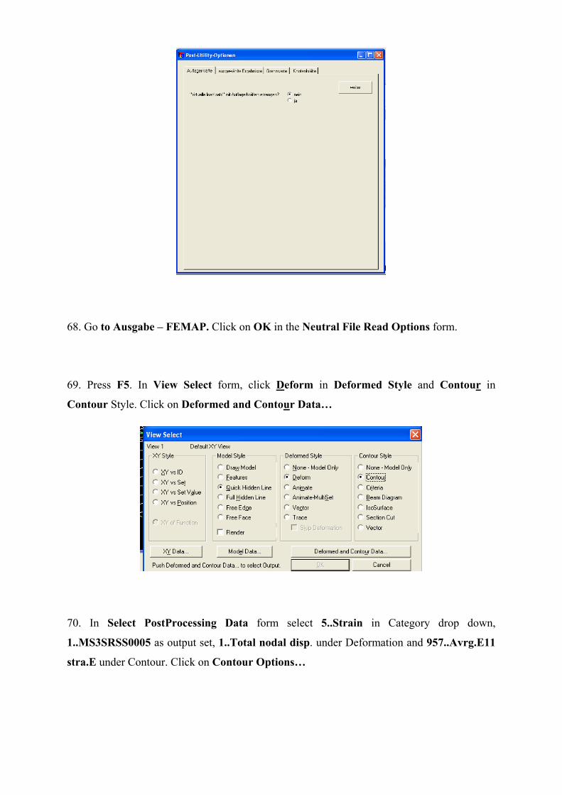
68. Go to Ausgabe – FEMAP. Click on OK in the Neutral File Read Options form.
69. Press F5. In View Select form, click Deform in Deformed Style and Contour in
Contour Style. Click on Deformed and Contour Data…
70. In Select PostProcessing Data form select 5..Strain in Category drop down,
1..MS3SRSS0005 as output set, 1..Total nodal disp. under Deformation and 957..Avrg.E11
stra.E under Contour. Click on Contour Options…
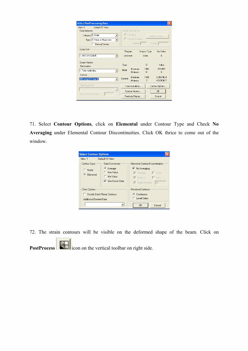
71. Select Contour Options, click on Elemental under Contour Type and Check No
Averaging under Elemental Contour Discontinuities. Click OK thrice to come out of the
window.
72. The strain contours will be visible on the deformed shape of the beam. Click on
PostProcess icon on the vertical toolbar on right side.
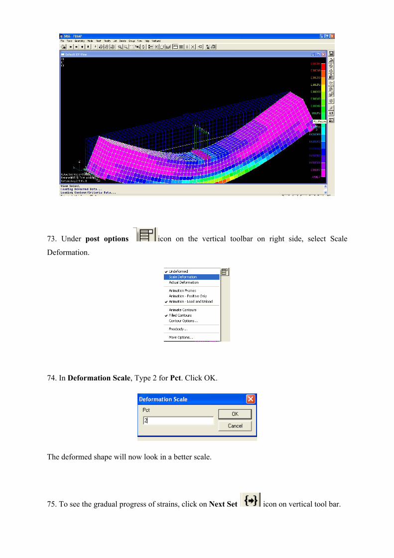
73. Under post options icon on the vertical toolbar on right side, select Scale
Deformation.
74. In Deformation Scale, Type 2 for Pct. Click OK.
The deformed shape will now look in a better scale.
75. To see the gradual progress of strains, click on Next Set icon on vertical tool bar.
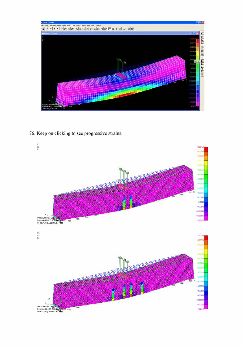
76. Keep on clicking to see progressive strains.
XY
Z
X
-700.-600.
-500.-400.
-300.-200.
-100.0.
100.200.
300.400.
500.600.
700.
Y
0.
3
1.1.1.1.1.1.1.
1313131313131313131313123123
0.00759
0.00711
0.00664
0.00616
0.00569
0.00522
0.00474
0.00427
0.00379
0.00332
0.00285
0.00237
0.0019
0.00142
0.000949
0.000475
6.93E-7
V1L1C1
Output Set: MS3 SRSS0015Deformed(1.627): Total nodal disp.Contour: Avrg.E11 stra. E
XY
Z
X
-700.-600.
-500.-400.
-300.-200.
-100.0.
100.200.
300.400.
500.600.
700.
Y
0.
3
1.1.1.1.1.1.1.
1313131313131313131313123123
0.0075
0.00704
0.00657
0.0061
0.00563
0.00516
0.00469
0.00422
0.00375
0.00328
0.00281
0.00235
0.00188
0.00141
0.000939
0.00047
7.11E-7
V1L1C1
Output Set: MS3 SRSS0020Deformed(2.139): Total nodal disp.Contour: Avrg.E11 stra. E
XY
Z
X
-700.-600.
-500.-400.
-300.-200.
-100.0.
100.200.
300.400.
500.600.
700.
Y
0.
3
1.1.1.1.1.1.1.
1313131313131313131313123123
0.0113
0.0106
0.00993
0.00922
0.00851
0.0078
0.00709
0.00638
0.00567
0.00496
0.00425
0.00355
0.00284
0.00213
0.00142
0.00071
8.66E-7
V1L1C1
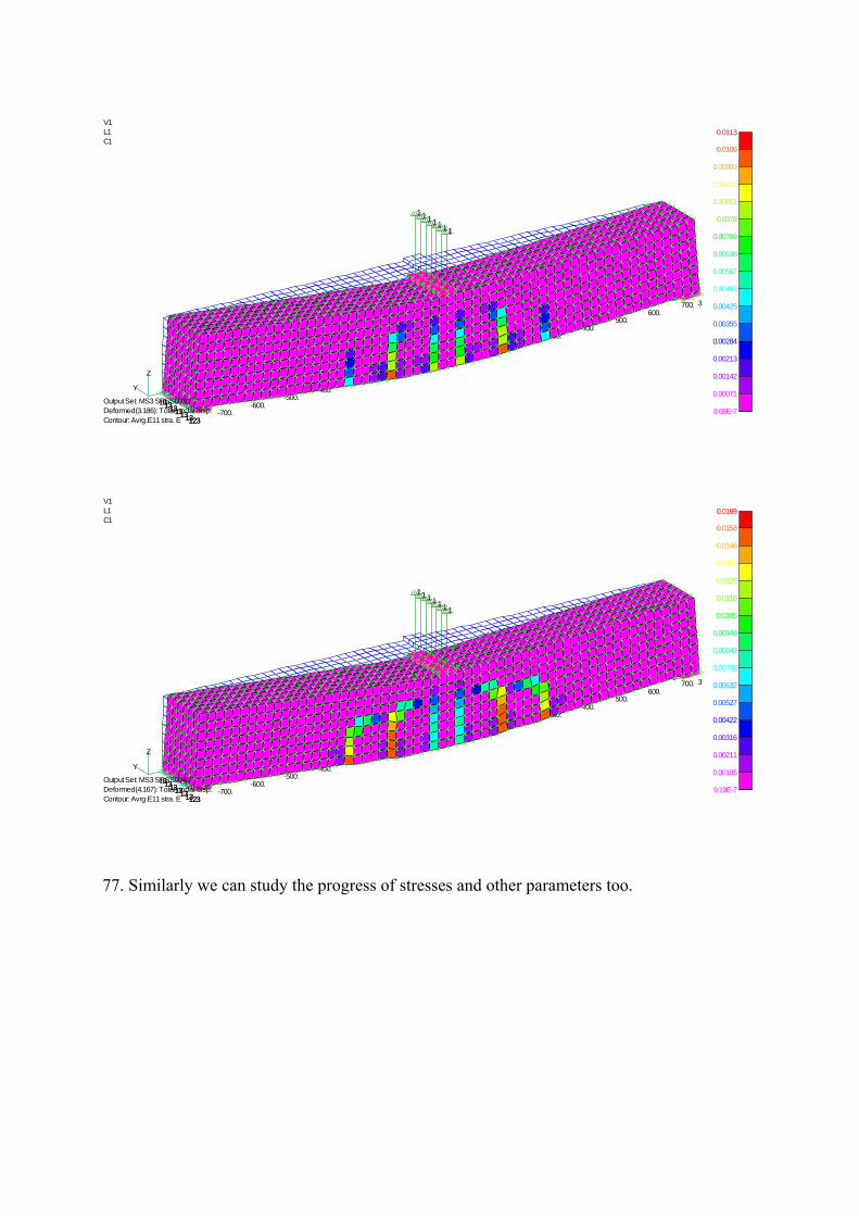
Output Set: MS3 SRSS0030Deformed(3.186): Total nodal disp.Contour: Avrg.E11 stra. E
XY
Z
X
-700.-600.
-500.-400.
-300.-200.
-100.0.
100.200.
300.400.
500.600.
700.
Y
0.
3
1.1.1.1.1.1.1.
1313131313131313131313123123
0.0169
0.0158
0.0148
0.0137
0.0126
0.0116
0.0105
0.00949
0.00843
0.00738
0.00632
0.00527
0.00422
0.00316
0.00211
0.00105
9.19E-7
V1L1C1
Output Set: MS3 SRSS0040Deformed(4.167): Total nodal disp.Contour: Avrg.E11 stra. E
77. Similarly we can study the progress of stresses and other parameters too.

TUTORIAL 3
ANALYSIS OF CANTILEVER BEAM WITH STIRRUPS AND BOND
ELEMENTS SUBJECTED TO CYCLIC LOAD AT FREE END
(Input files available under name :example3.ms3)
In this tutorial, you will learn
1. Modeling of Stirrups
2. Modeling of Bond Elements
3. Perform Cyclic Analysis
4. Working with half model to save time
5. Playing with Colors of Elements, Layers etc for Better Control over Model
6. Viewing Output Results in Presentable Format
7. Making Animations of output results
Problem Statement:
To perform cyclic analysis of a realistic reinforced concrete beam with stirrups and
longitudinal reinforcement in top and bottom designed for gravity type loading with top bars
bent in and bottom bars straight as shown in the figure. To consider the embedment of
longitudinal bars, a stub is assumed that may be visualized as a part of the column of the
beam-column joint.
The details for the beam are given below.
Compressive strength of concrete = 25 MPa
Tensile strength of concrete = 2.5 MPa
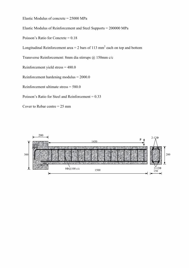
Elastic Modulus of concrete = 25000 MPa
Elastic Modulus of Reinforcement and Steel Supports = 200000 MPa
Poisson’s Ratio for Concrete = 0.18
Longitudinal Reinforcement area = 2 bars of 113 mm2 each on top and bottom
Transverse Reinforcement: 8mm dia stirrups @ 150mm c/c
Reinforcement yield stress = 480.0
Reinforcement hardening modulus = 2000.0
Reinforcement ultimate stress = 580.0
Poisson’s Ratio for Steel and Reinforcement = 0.33
Cover to Rebar centre = 25 mm
1450 P
150
200
8Φ@100 c/c 2-12Φ
200
300
2-12Φ
1500
100
25 25

STEPS TO BE FOLLOWED
1. Open MASA to get the MASA Main screen.
2. Go to Projekt – Neues Projekt. Give path for the project folder. Write Cantilever in
projektname. Complete path will be shown in Projekt bar. ! The complete path length
must be kept under 50 characters.
3. Go to Eingabe – FEMAP. After the FEMAP Flash screen, and error message will
appear stating “Unable to Open File TB.PRG: No such file or directory”. Click OK
4. Go to Geometry – Solid – Primitives. In the Solid Primitives Window, give SRSS as
Title and type 1500, 150 and 200 for X, Y and Z respectively. Click OK.
5. Window showing the beam in Default XY View will appear. Click on Dyn Rotate
button to rotate the model and obtain desirable view. (It is advised to keep Z axis as
vertical upwards).
6. Press Ctrl + Q to get View Quick Options dialog box. Under the Geometry column,
uncheck the Surface and Volume Check boxes. Click Done. Now we will be able to
see only boundary lines of the beam.
7. Again go to Geometry – Solid – Primitives. In the Solid Primitives Window, click on
new solid and type 200, 150 and 300 for X, Y and Z respectively. You may write
Stub in the title. Click OK.
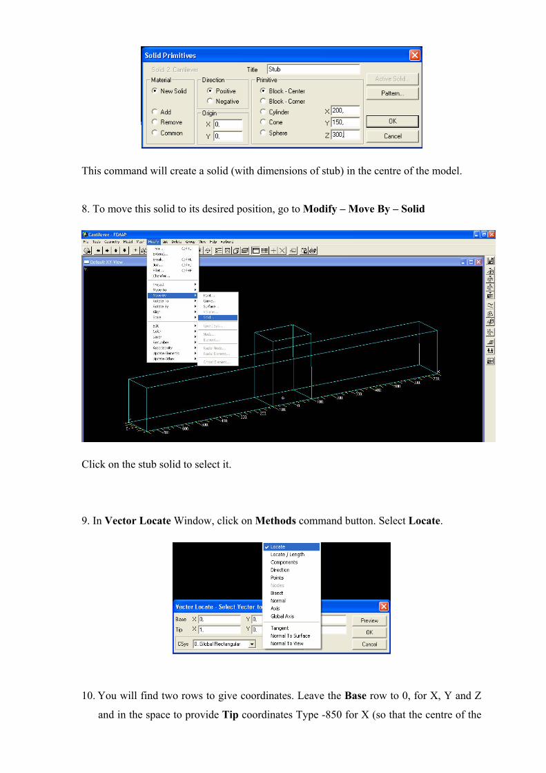
This command will create a solid (with dimensions of stub) in the centre of the model.
8. To move this solid to its desired position, go to Modify – Move By – Solid
Click on the stub solid to select it.
9. In Vector Locate Window, click on Methods command button. Select Locate.
10. You will find two rows to give coordinates. Leave the Base row to 0, for X, Y and Z
and in the space to provide Tip coordinates Type -850 for X (so that the centre of the
stub comes to 100 mm beyond the beam as we desire), leave Y as 0, (since we do not
want to move the solid in Y direction) and type -50 for Z so that the stub is moved by
50mm in the downwards direction.
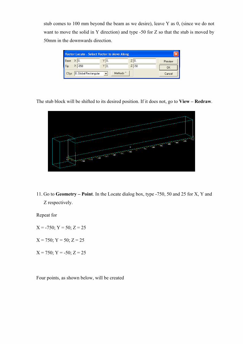
The stub block will be shifted to its desired position. If it does not, go to View – Redraw.
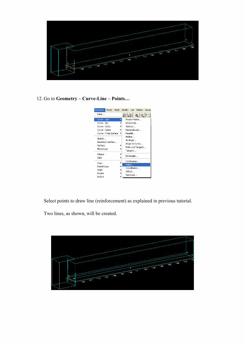
11. Go to Geometry – Point. In the Locate dialog box, type -750, 50 and 25 for X, Y and
Z respectively.
Repeat for
X = -750; Y = 50; Z = 25
X = 750; Y = 50; Z = 25
X = 750; Y = -50; Z = 25
Four points, as shown below, will be created
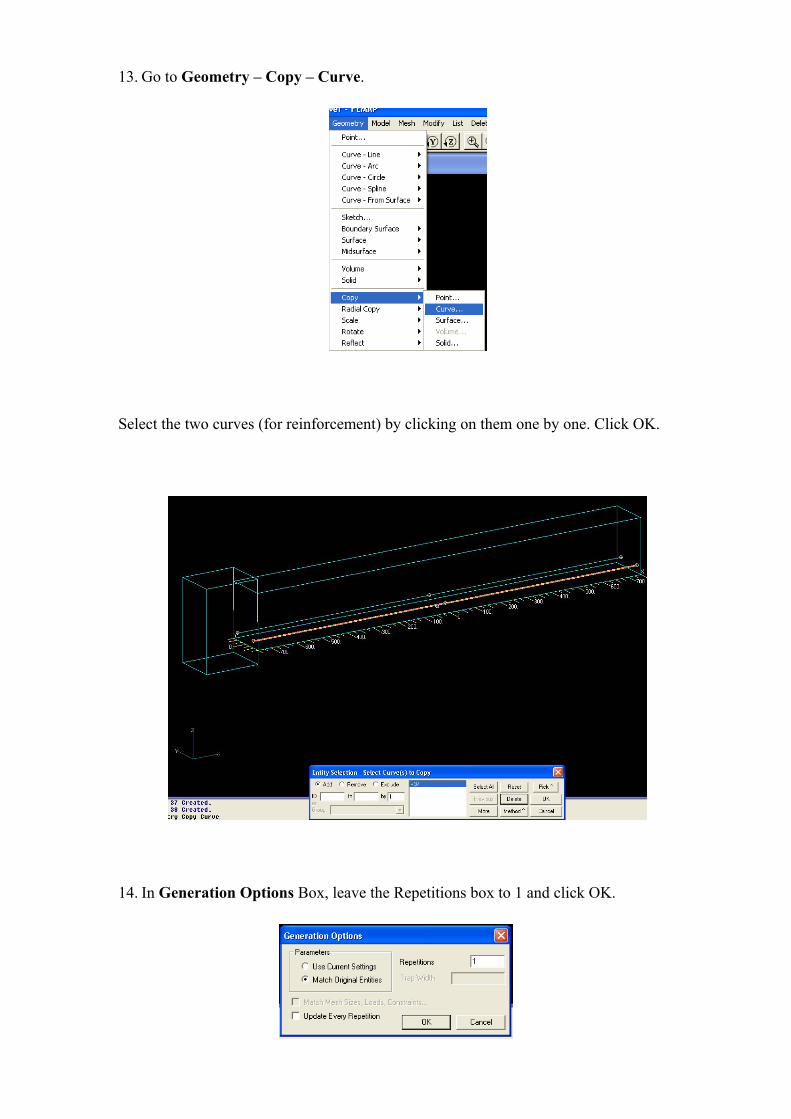
12. Go to Geometry – Curve-Line – Points…
Select points to draw line (reinforcement) as explained in previous tutorial.
Two lines, as shown, will be created.
13. Go to Geometry – Copy – Curve.
Select the two curves (for reinforcement) by clicking on them one by one. Click OK.
14. In Generation Options Box, leave the Repetitions box to 1 and click OK.
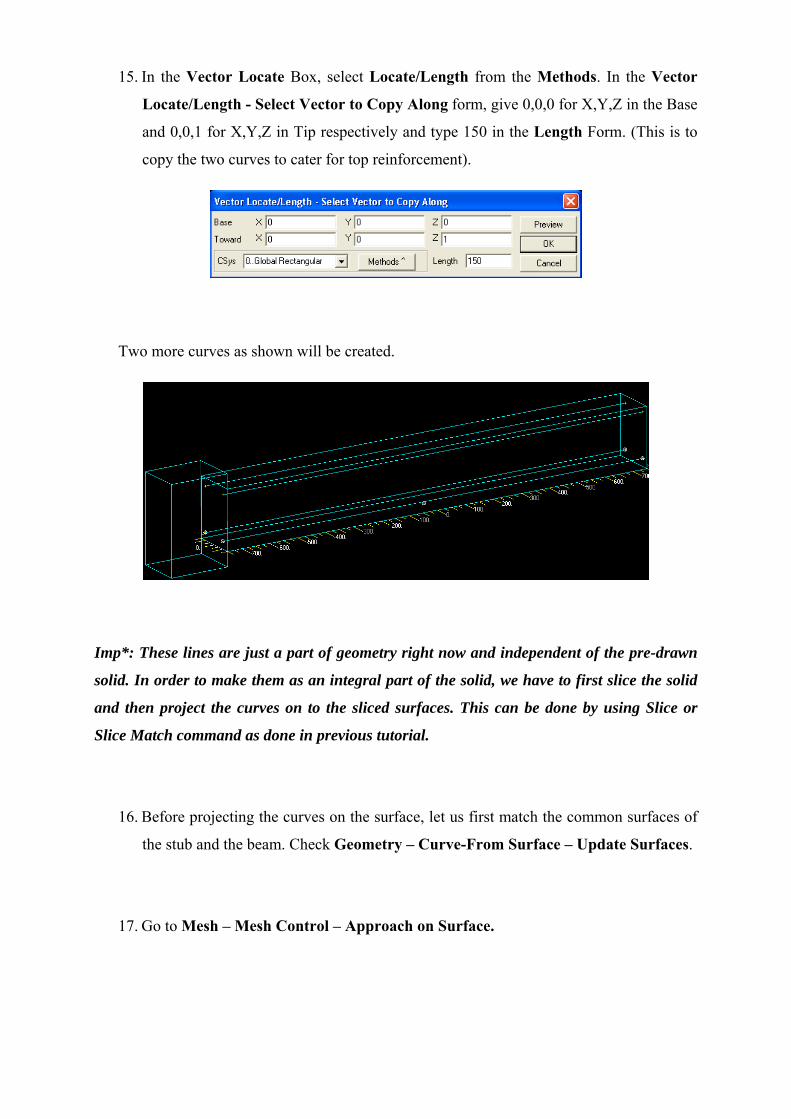
15. In the Vector Locate Box, select Locate/Length from the Methods. In the Vector
Locate/Length - Select Vector to Copy Along form, give 0,0,0 for X,Y,Z in the Base
and 0,0,1 for X,Y,Z in Tip respectively and type 150 in the Length Form. (This is to
copy the two curves to cater for top reinforcement).
Two more curves as shown will be created.
Imp*: These lines are just a part of geometry right now and independent of the pre-drawn
solid. In order to make them as an integral part of the solid, we have to first slice the solid
and then project the curves on to the sliced surfaces. This can be done by using Slice or
Slice Match command as done in previous tutorial.
16. Before projecting the curves on the surface, let us first match the common surfaces of
the stub and the beam. Check Geometry – Curve-From Surface – Update Surfaces.
17. Go to Mesh – Mesh Control – Approach on Surface.
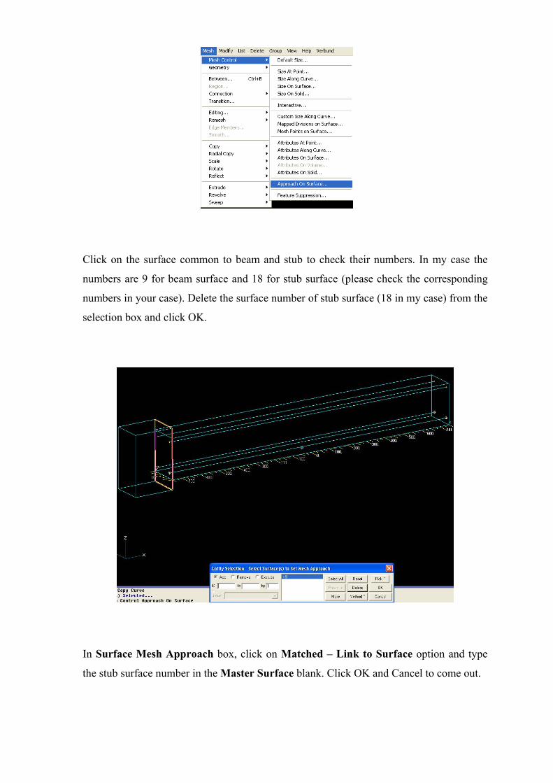
Click on the surface common to beam and stub to check their numbers. In my case the
numbers are 9 for beam surface and 18 for stub surface (please check the corresponding
numbers in your case). Delete the surface number of stub surface (18 in my case) from the
selection box and click OK.
In Surface Mesh Approach box, click on Matched – Link to Surface option and type
the stub surface number in the Master Surface blank. Click OK and Cancel to come out.
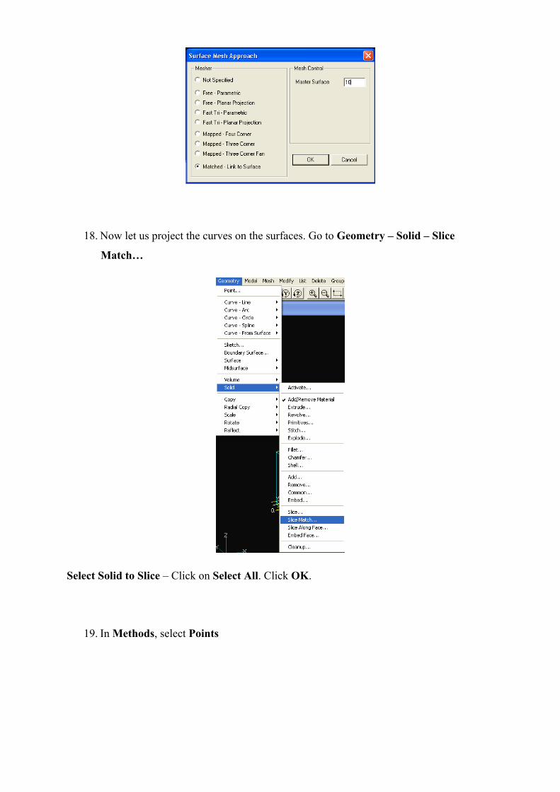
18. Now let us project the curves on the surfaces. Go to Geometry – Solid – Slice
Match…
Select Solid to Slice – Click on Select All. Click OK.
19. In Methods, select Points
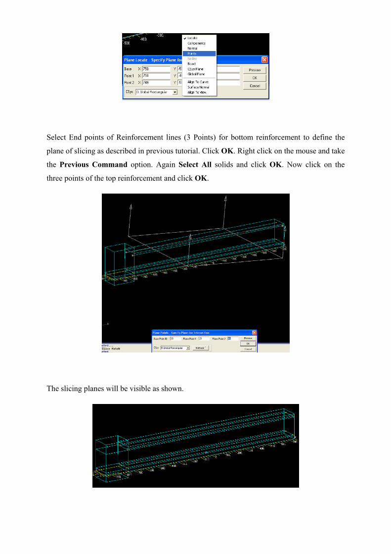
Select End points of Reinforcement lines (3 Points) for bottom reinforcement to define the
plane of slicing as described in previous tutorial. Click OK. Right click on the mouse and take
the Previous Command option. Again Select All solids and click OK. Now click on the
three points of the top reinforcement and click OK.
The slicing planes will be visible as shown.
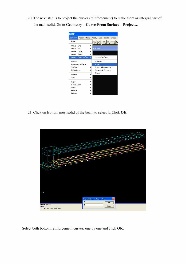
20. The next step is to project the curves (reinforcement) to make them as integral part of
the main solid. Go to Geometry – Curve-From Surface – Project…
21. Click on Bottom most solid of the beam to select it. Click OK.
Select both bottom reinforcement curves, one by one and click OK.
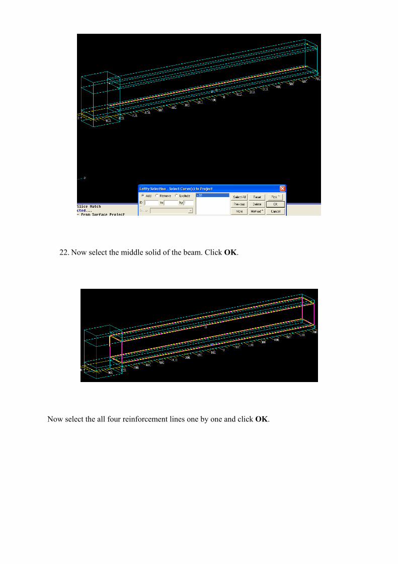
22. Now select the middle solid of the beam. Click OK.
Now select the all four reinforcement lines one by one and click OK.
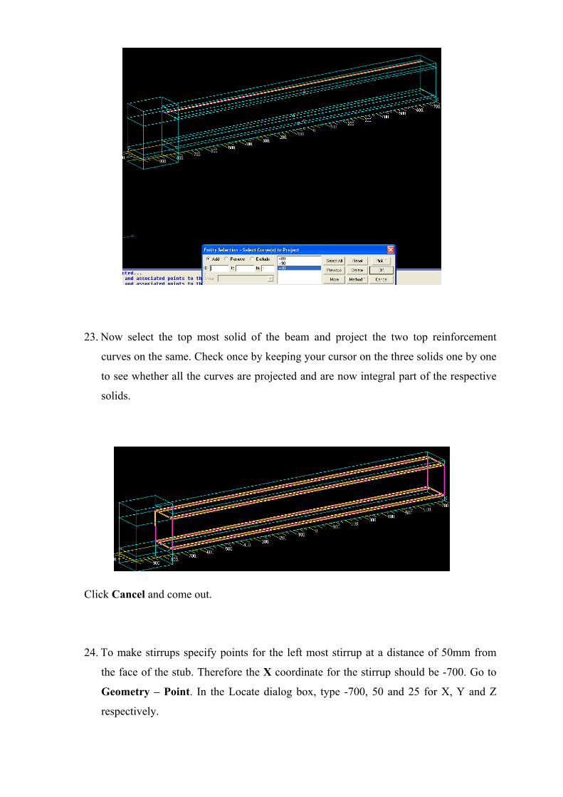
23. Now select the top most solid of the beam and project the two top reinforcement
curves on the same. Check once by keeping your cursor on the three solids one by one
to see whether all the curves are projected and are now integral part of the respective
solids.
Click Cancel and come out.
24. To make stirrups specify points for the left most stirrup at a distance of 50mm from
the face of the stub. Therefore the X coordinate for the stirrup should be -700. Go to
Geometry – Point. In the Locate dialog box, type -700, 50 and 25 for X, Y and Z
respectively.
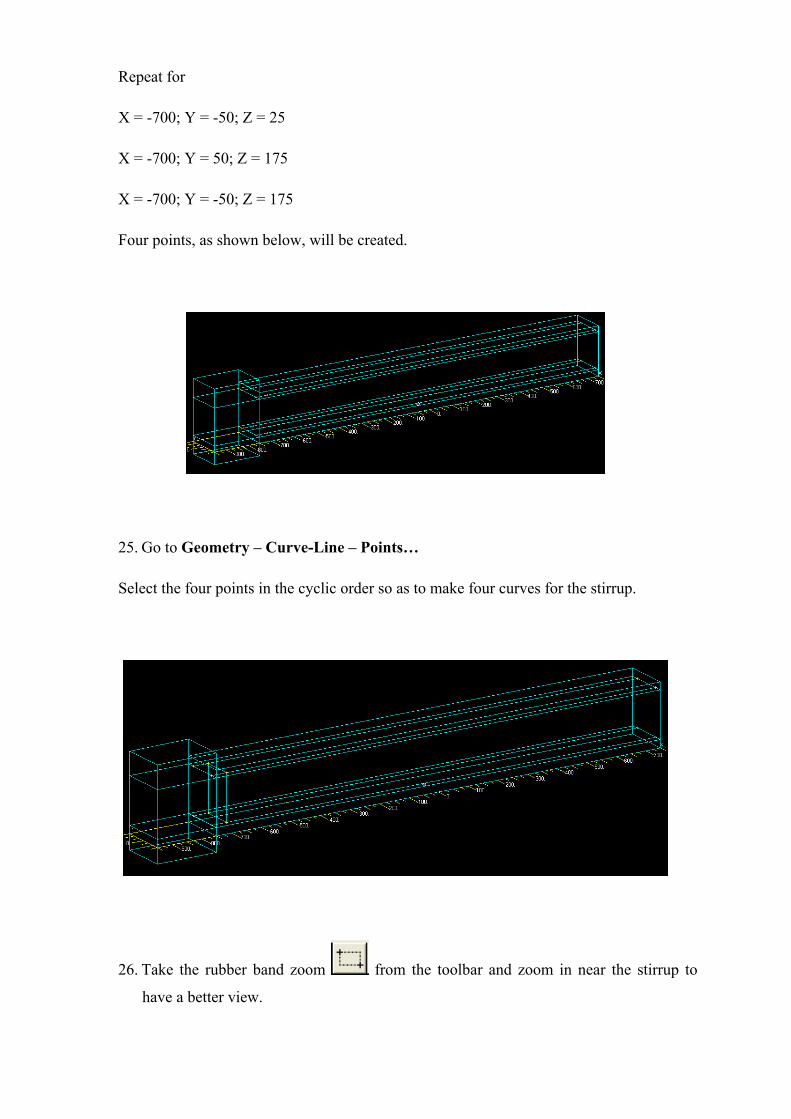
Repeat for
X = -700; Y = -50; Z = 25
X = -700; Y = 50; Z = 175
X = -700; Y = -50; Z = 175
Four points, as shown below, will be created.
25. Go to Geometry – Curve-Line – Points…
Select the four points in the cyclic order so as to make four curves for the stirrup.
26. Take the rubber band zoom from the toolbar and zoom in near the stirrup to
have a better view.
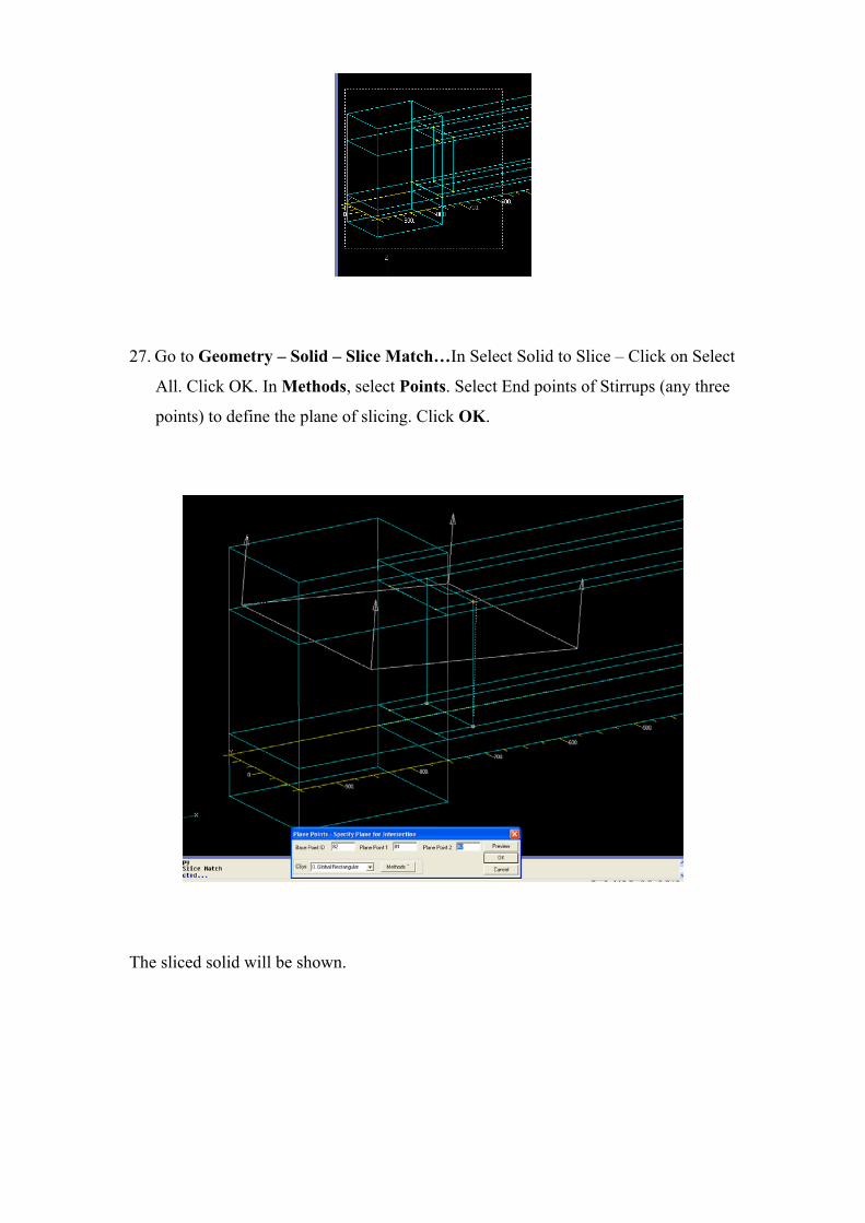
27. Go to Geometry – Solid – Slice Match…In Select Solid to Slice – Click on Select
All. Click OK. In Methods, select Points. Select End points of Stirrups (any three
points) to define the plane of slicing. Click OK.
The sliced solid will be shown.
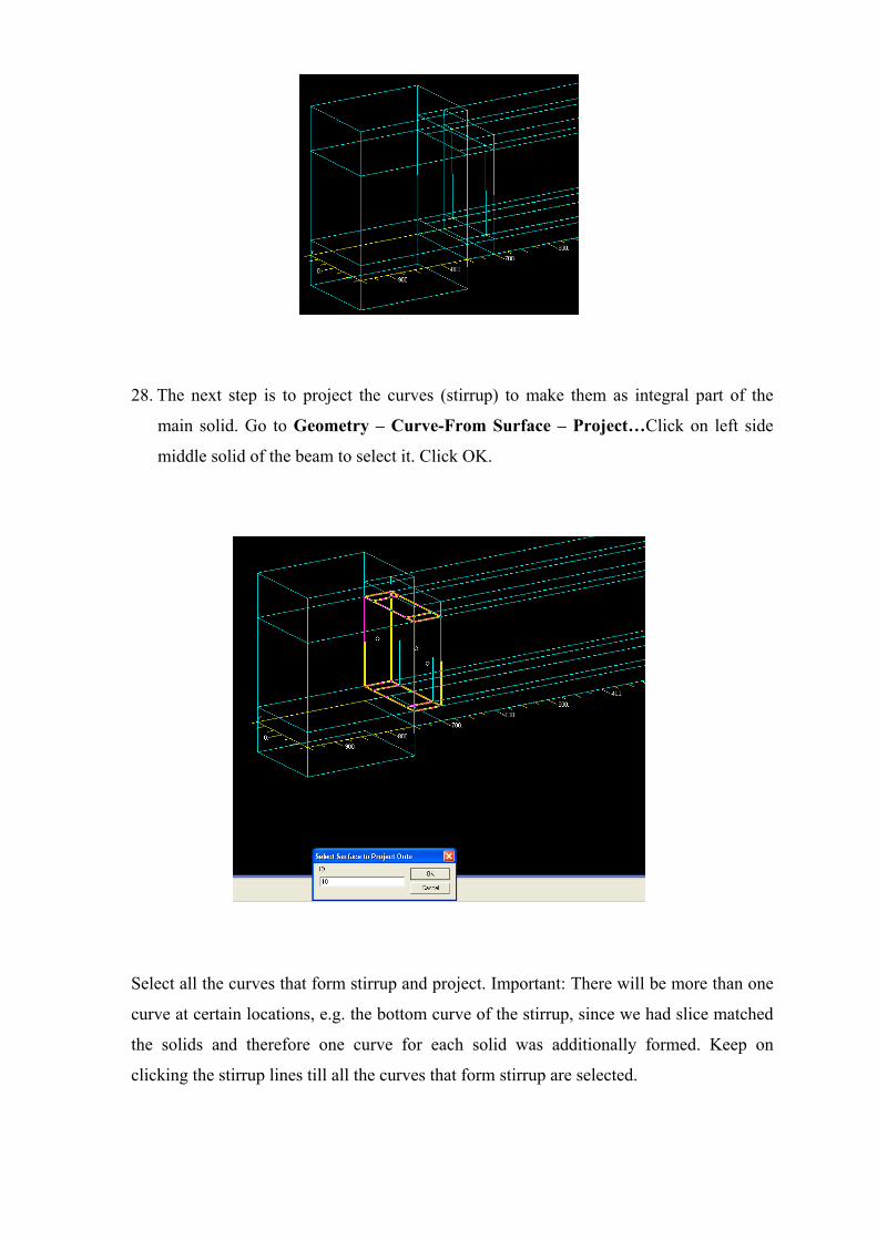
28. The next step is to project the curves (stirrup) to make them as integral part of the
main solid. Go to Geometry – Curve-From Surface – Project…Click on left side
middle solid of the beam to select it. Click OK.
Select all the curves that form stirrup and project. Important: There will be more than one
curve at certain locations, e.g. the bottom curve of the stirrup, since we had slice matched
the solids and therefore one curve for each solid was additionally formed. Keep on
clicking the stirrup lines till all the curves that form stirrup are selected.
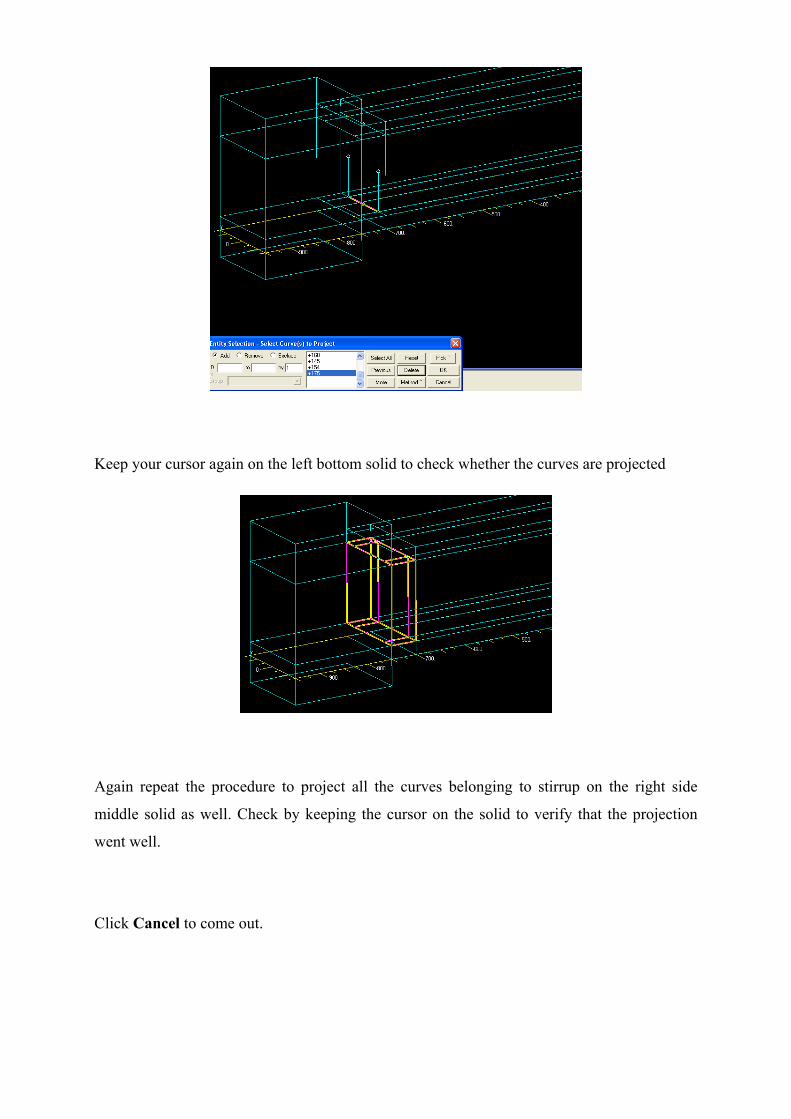
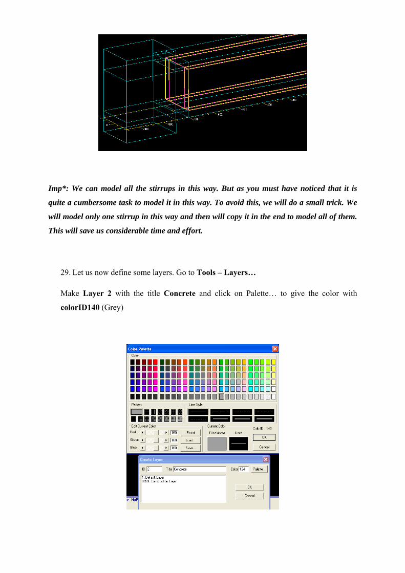
Keep your cursor again on the left bottom solid to check whether the curves are projected
Again repeat the procedure to project all the curves belonging to stirrup on the right side
middle solid as well. Check by keeping the cursor on the solid to verify that the projection
went well.
Click Cancel to come out.
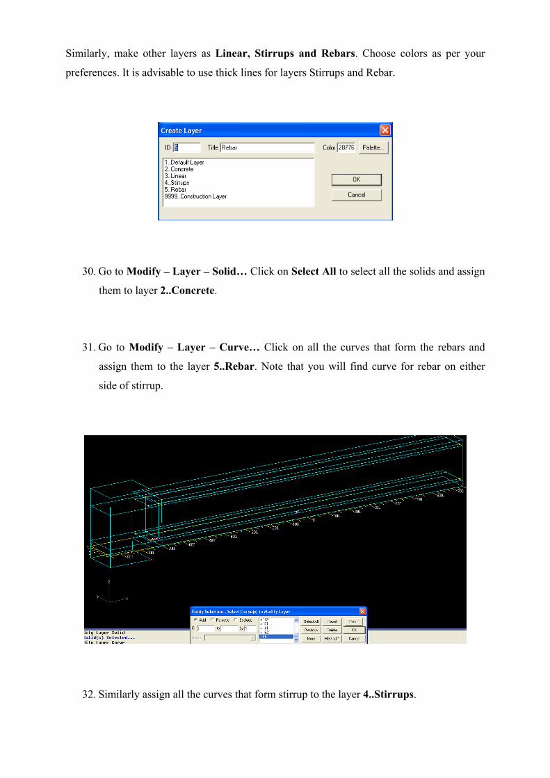
Imp*: We can model all the stirrups in this way. But as you must have noticed that it is
quite a cumbersome task to model it in this way. To avoid this, we will do a small trick. We
will model only one stirrup in this way and then will copy it in the end to model all of them.
This will save us considerable time and effort.
29. Let us now define some layers. Go to Tools – Layers…
Make Layer 2 with the title Concrete and click on Palette… to give the color with
colorID140 (Grey)
Similarly, make other layers as Linear, Stirrups and Rebars. Choose colors as per your
preferences. It is advisable to use thick lines for layers Stirrups and Rebar.
30. Go to Modify – Layer – Solid… Click on Select All to select all the solids and assign
them to layer 2..Concrete.
31. Go to Modify – Layer – Curve… Click on all the curves that form the rebars and
assign them to the layer 5..Rebar. Note that you will find curve for rebar on either
side of stirrup.
32. Similarly assign all the curves that form stirrup to the layer 4..Stirrups.
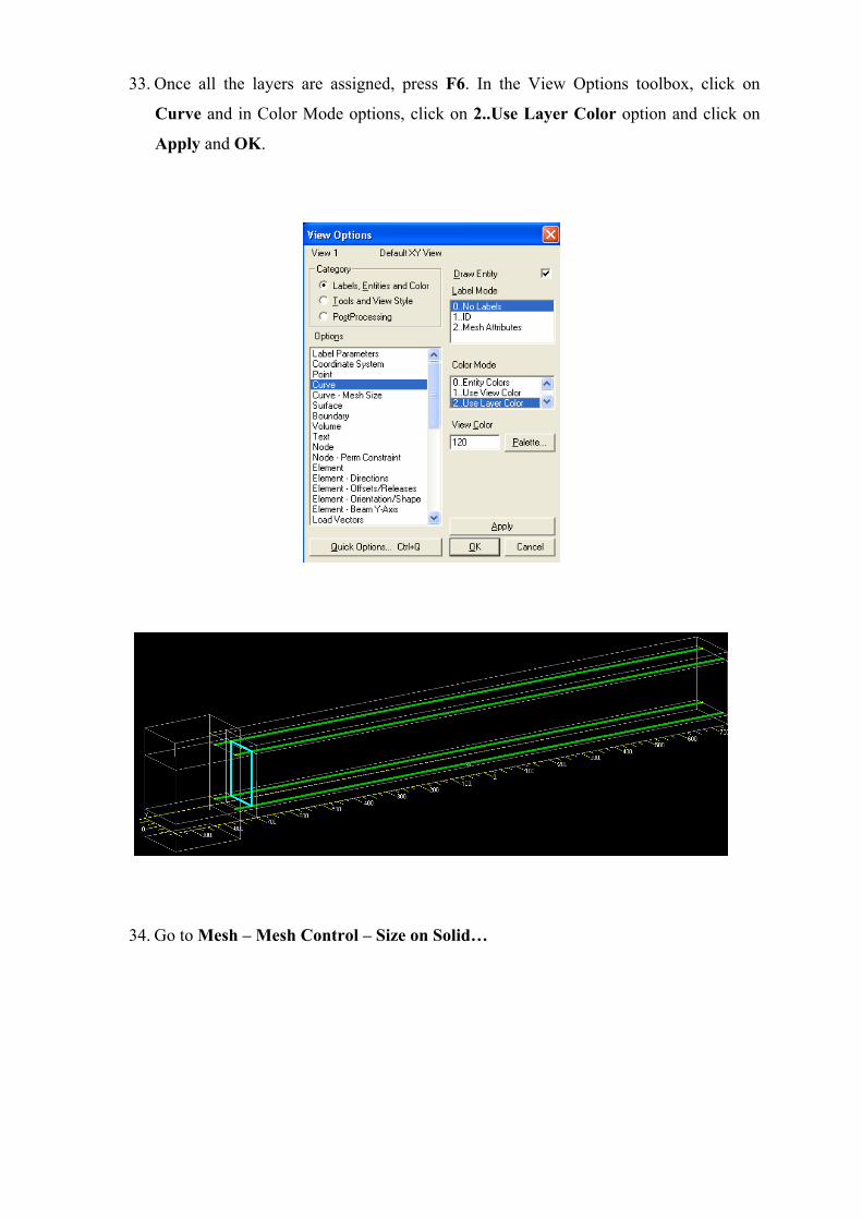
33. Once all the layers are assigned, press F6. In the View Options toolbox, click on
Curve and in Color Mode options, click on 2..Use Layer Color option and click on
Apply and OK.
34. Go to Mesh – Mesh Control – Size on Solid…
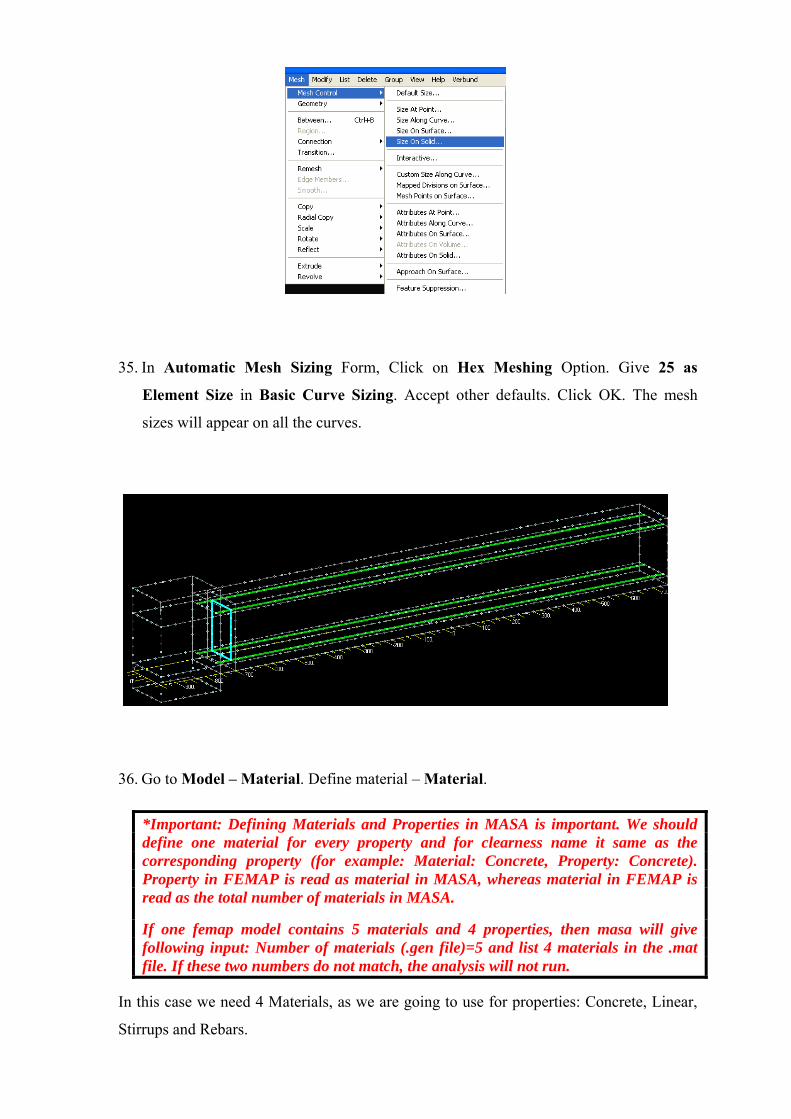
35. In Automatic Mesh Sizing Form, Click on Hex Meshing Option. Give 25 as
Element Size in Basic Curve Sizing. Accept other defaults. Click OK. The mesh
sizes will appear on all the curves.
36. Go to Model – Material. Define material – Material.
*Important: Defining Materials and Properties in MASA is important. We should define one material for every property and for clearness name it same as the corresponding property (for example: Material: Concrete, Property: Concrete). Property in FEMAP is read as material in MASA, whereas material in FEMAP is read as the total number of materials in MASA.
If one femap model contains 5 materials and 4 properties, then masa will give following input: Number of materials (.gen file)=5 and list 4 materials in the .mat file. If these two numbers do not match, the analysis will not run.
In this case we need 4 Materials, as we are going to use for properties: Concrete, Linear,
Stirrups and Rebars.
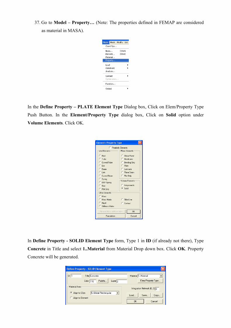
37. Go to Model – Property… (Note: The properties defined in FEMAP are considered
as material in MASA).
In the Define Property – PLATE Element Type Dialog box, Click on Elem/Property Type
Push Button. In the Element/Property Type dialog box, Click on Solid option under
Volume Elements. Click OK.
In Define Property - SOLID Element Type form, Type 1 in ID (if already not there), Type
Concrete in Title and select 1..Material from Material Drop down box. Click OK. Property
Concrete will be generated.
Similarly, create property 2 as Linear (solid), property 3 as Stirrups (bar) and property 4 as
Rebar (bar).
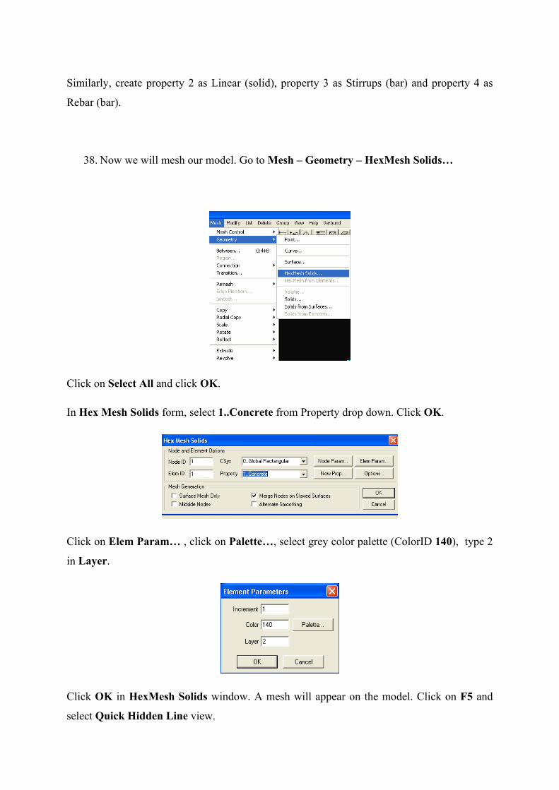
38. Now we will mesh our model. Go to Mesh – Geometry – HexMesh Solids…
Click on Select All and click OK.
In Hex Mesh Solids form, select 1..Concrete from Property drop down. Click OK.
Click on Elem Param… , click on Palette…, select grey color palette (ColorID 140), type 2
in Layer.
Click OK in HexMesh Solids window. A mesh will appear on the model. Click on F5 and
select Quick Hidden Line view.
Again click on F5 and make the view to Draw Model, else we will not be able to view the
curves later.
39. Since we have already assigned the solids, curves and elements to the respective
layers, we can now hide concrete layer and see only the reinforcement curves. If you
might have forgotten to do so, you may assign all elements to layer concrete by using
Modify – Layer – Element command.
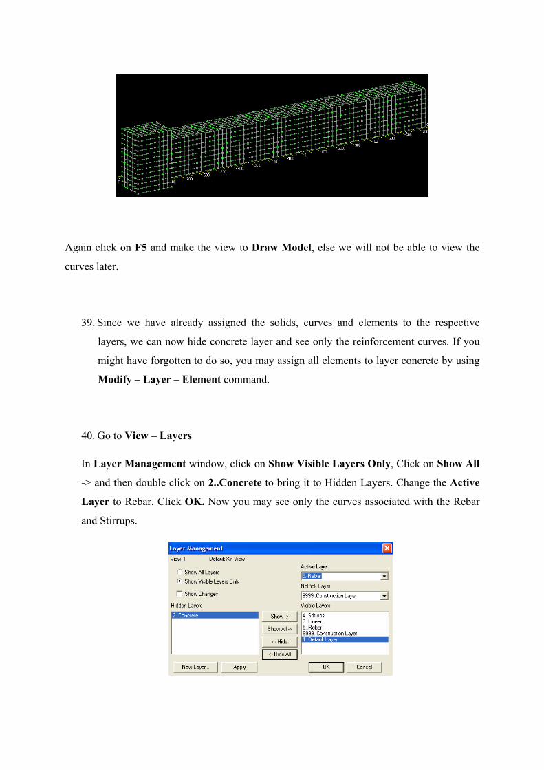
40. Go to View – Layers
In Layer Management window, click on Show Visible Layers Only, Click on Show All
-> and then double click on 2..Concrete to bring it to Hidden Layers. Change the Active
Layer to Rebar. Click OK. Now you may see only the curves associated with the Rebar
and Stirrups.
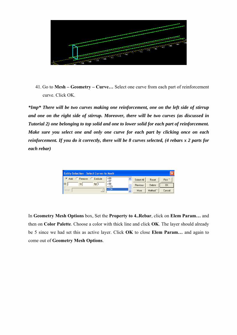
41. Go to Mesh – Geometry – Curve… Select one curve from each part of reinforcement
curve. Click OK.
*Imp* There will be two curves making one reinforcement, one on the left side of stirrup
and one on the right side of stirrup. Moreover, there will be two curves (as discussed in
Tutorial 2) one belonging to top solid and one to lower solid for each part of reinforcement.
Make sure you select one and only one curve for each part by clicking once on each
reinforcement. If you do it correctly, there will be 8 curves selected, (4 rebars x 2 parts for
each rebar)
In Geometry Mesh Options box, Set the Property to 4..Rebar, click on Elem Param… and
then on Color Palette. Choose a color with thick line and click OK. The layer should already
be 5 since we had set this as active layer. Click OK to close Elem Param… and again to
come out of Geometry Mesh Options.
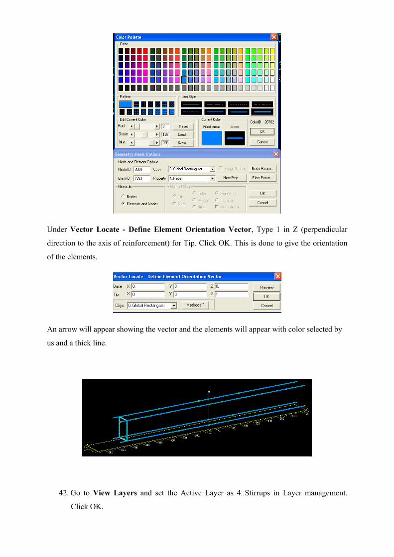
Under Vector Locate - Define Element Orientation Vector, Type 1 in Z (perpendicular
direction to the axis of reinforcement) for Tip. Click OK. This is done to give the orientation
of the elements.
An arrow will appear showing the vector and the elements will appear with color selected by
us and a thick line.
42. Go to View Layers and set the Active Layer as 4..Stirrups in Layer management.
Click OK.
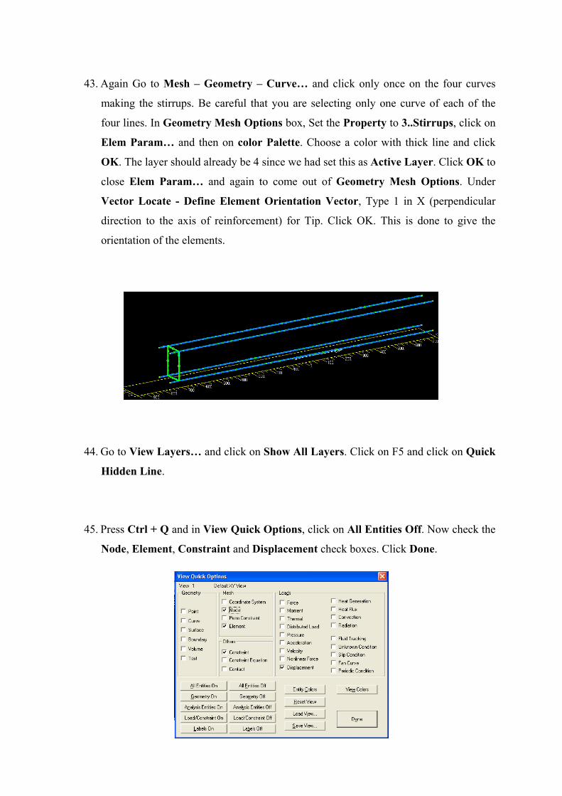
43. Again Go to Mesh – Geometry – Curve… and click only once on the four curves
making the stirrups. Be careful that you are selecting only one curve of each of the
four lines. In Geometry Mesh Options box, Set the Property to 3..Stirrups, click on
Elem Param… and then on color Palette. Choose a color with thick line and click
OK. The layer should already be 4 since we had set this as Active Layer. Click OK to
close Elem Param… and again to come out of Geometry Mesh Options. Under
Vector Locate - Define Element Orientation Vector, Type 1 in X (perpendicular
direction to the axis of reinforcement) for Tip. Click OK. This is done to give the
orientation of the elements.
44. Go to View Layers… and click on Show All Layers. Click on F5 and click on Quick
Hidden Line.
45. Press Ctrl + Q and in View Quick Options, click on All Entities Off. Now check the
Node, Element, Constraint and Displacement check boxes. Click Done.
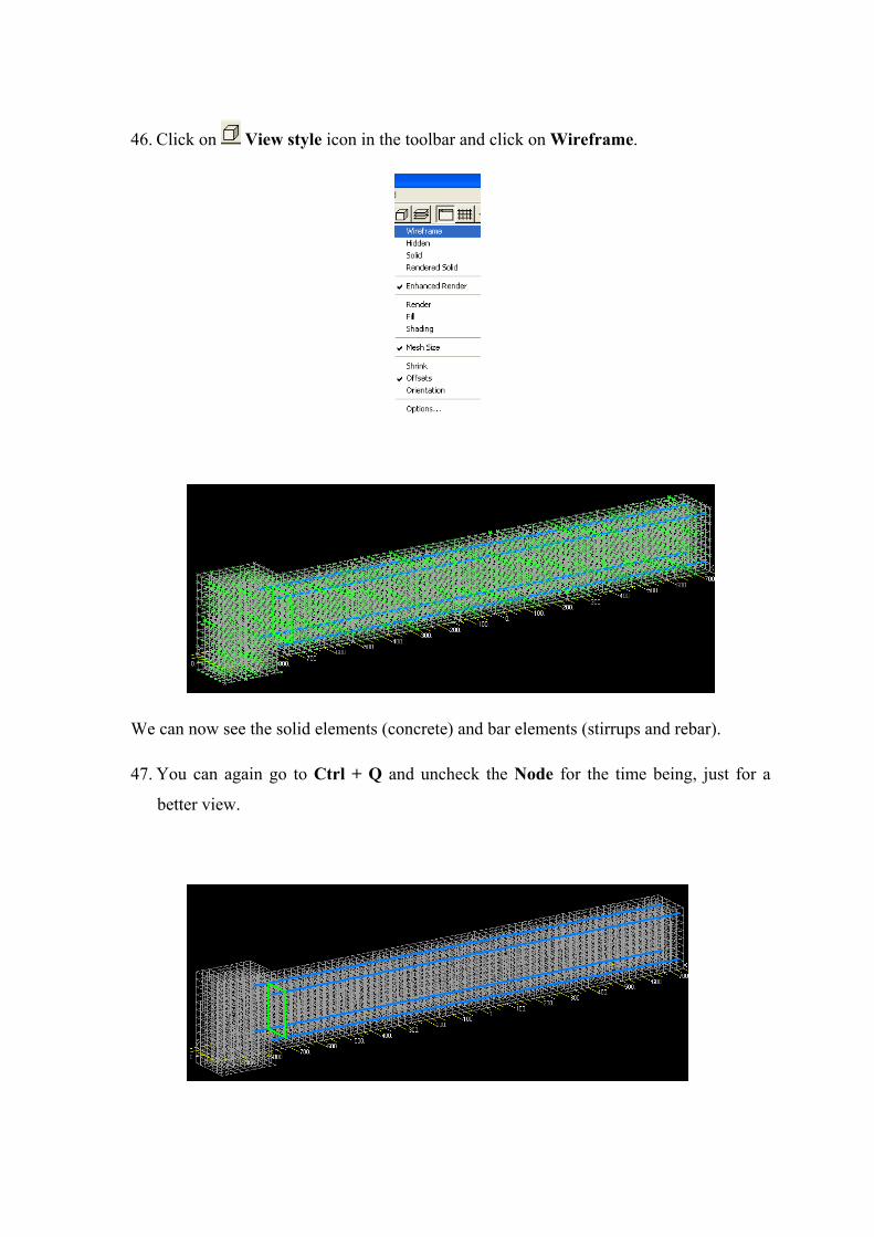
46. Click on View style icon in the toolbar and click on Wireframe.
We can now see the solid elements (concrete) and bar elements (stirrups and rebar).
47. You can again go to Ctrl + Q and uncheck the Node for the time being, just for a
better view.
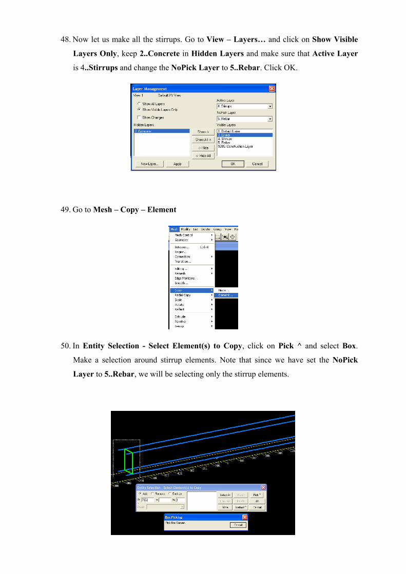
48. Now let us make all the stirrups. Go to View – Layers… and click on Show Visible
Layers Only, keep 2..Concrete in Hidden Layers and make sure that Active Layer
is 4..Stirrups and change the NoPick Layer to 5..Rebar. Click OK.
49. Go to Mesh – Copy – Element
50. In Entity Selection - Select Element(s) to Copy, click on Pick ^ and select Box.
Make a selection around stirrup elements. Note that since we have set the NoPick
Layer to 5..Rebar, we will be selecting only the stirrup elements.
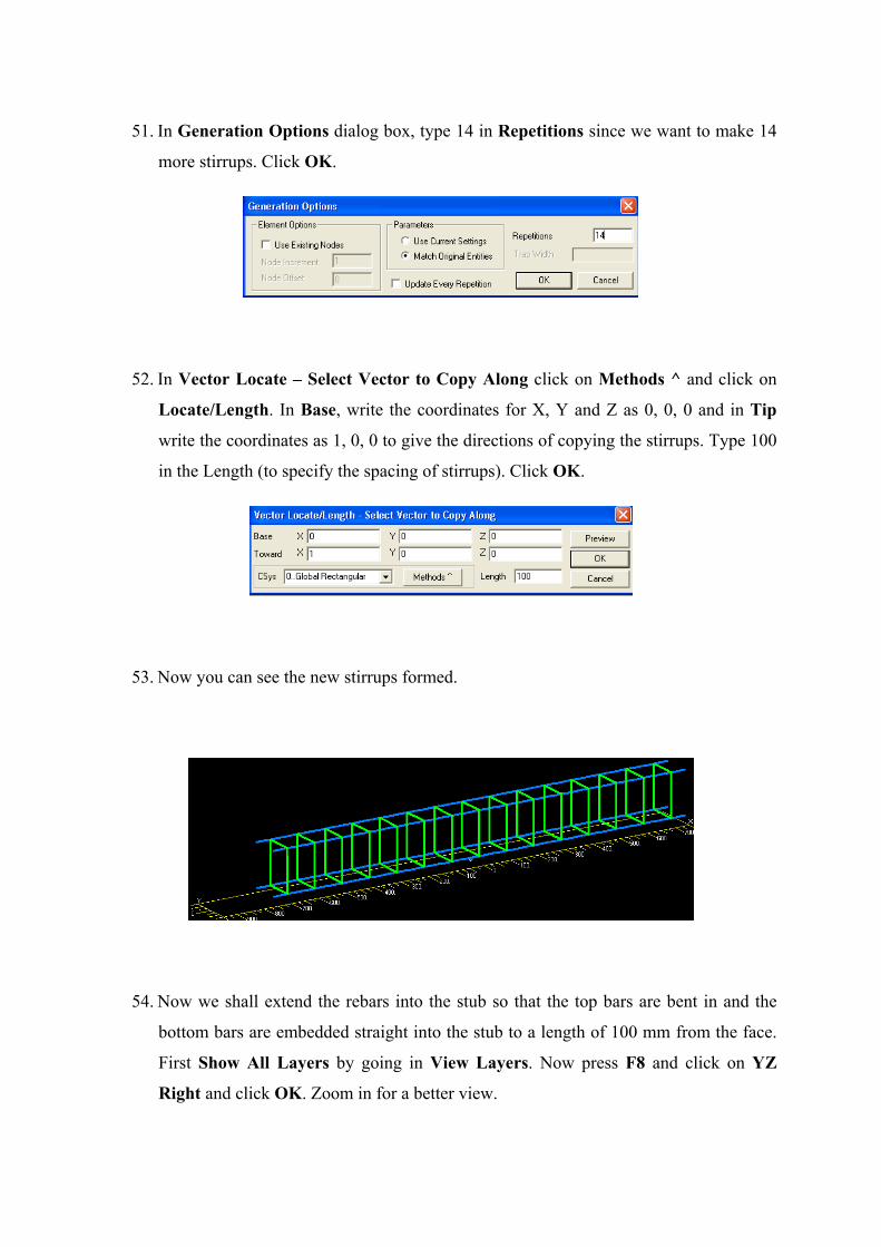
51. In Generation Options dialog box, type 14 in Repetitions since we want to make 14
more stirrups. Click OK.
52. In Vector Locate – Select Vector to Copy Along click on Methods ^ and click on
Locate/Length. In Base, write the coordinates for X, Y and Z as 0, 0, 0 and in Tip
write the coordinates as 1, 0, 0 to give the directions of copying the stirrups. Type 100
in the Length (to specify the spacing of stirrups). Click OK.
53. Now you can see the new stirrups formed.
54. Now we shall extend the rebars into the stub so that the top bars are bent in and the
bottom bars are embedded straight into the stub to a length of 100 mm from the face.
First Show All Layers by going in View Layers. Now press F8 and click on YZ
Right and click OK. Zoom in for a better view.
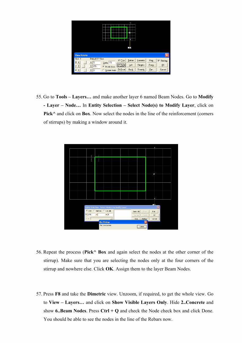
55. Go to Tools – Layers… and make another layer 6 named Beam Nodes. Go to Modify
- Layer – Node… In Entity Selection – Select Node(s) to Modify Layer, click on
Pick^ and click on Box. Now select the nodes in the line of the reinforcement (corners
of stirrups) by making a window around it.
56. Repeat the process (Pick^ Box and again select the nodes at the other corner of the
stirrup). Make sure that you are selecting the nodes only at the four corners of the
stirrup and nowhere else. Click OK. Assign them to the layer Beam Nodes.
57. Press F8 and take the Dimetric view. Unzoom, if required, to get the whole view. Go
to View – Layers… and click on Show Visible Layers Only. Hide 2..Concrete and
show 6..Beam Nodes. Press Ctrl + Q and check the Node check box and click Done.
You should be able to see the nodes in the line of the Rebars now.
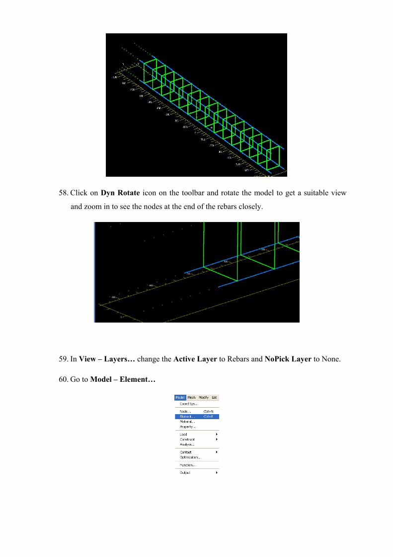
58. Click on Dyn Rotate icon on the toolbar and rotate the model to get a suitable view
and zoom in to see the nodes at the end of the rebars closely.
59. In View – Layers… change the Active Layer to Rebars and NoPick Layer to None.
60. Go to Model – Element…
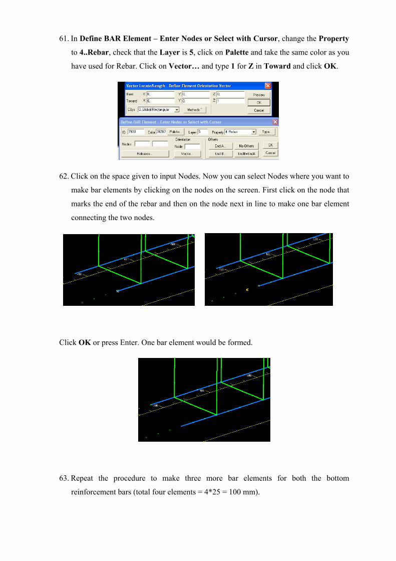
61. In Define BAR Element – Enter Nodes or Select with Cursor, change the Property
to 4..Rebar, check that the Layer is 5, click on Palette and take the same color as you
have used for Rebar. Click on Vector… and type 1 for Z in Toward and click OK.
62. Click on the space given to input Nodes. Now you can select Nodes where you want to
make bar elements by clicking on the nodes on the screen. First click on the node that
marks the end of the rebar and then on the node next in line to make one bar element
connecting the two nodes.
Click OK or press Enter. One bar element would be formed.
63. Repeat the procedure to make three more bar elements for both the bottom
reinforcement bars (total four elements = 4*25 = 100 mm).
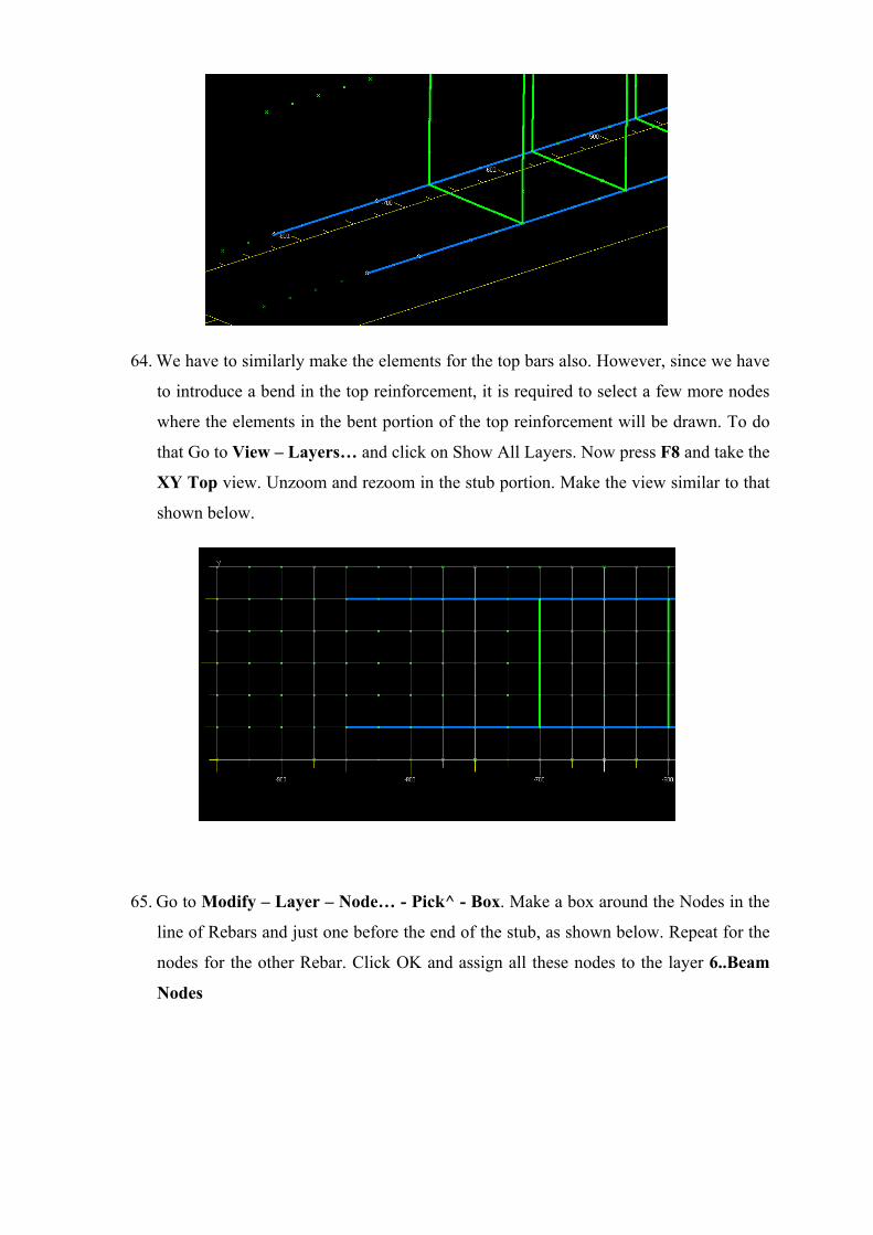
64. We have to similarly make the elements for the top bars also. However, since we have
to introduce a bend in the top reinforcement, it is required to select a few more nodes
where the elements in the bent portion of the top reinforcement will be drawn. To do
that Go to View – Layers… and click on Show All Layers. Now press F8 and take the
XY Top view. Unzoom and rezoom in the stub portion. Make the view similar to that
shown below.
65. Go to Modify – Layer – Node… - Pick^ - Box. Make a box around the Nodes in the
line of Rebars and just one before the end of the stub, as shown below. Repeat for the
nodes for the other Rebar. Click OK and assign all these nodes to the layer 6..Beam
Nodes
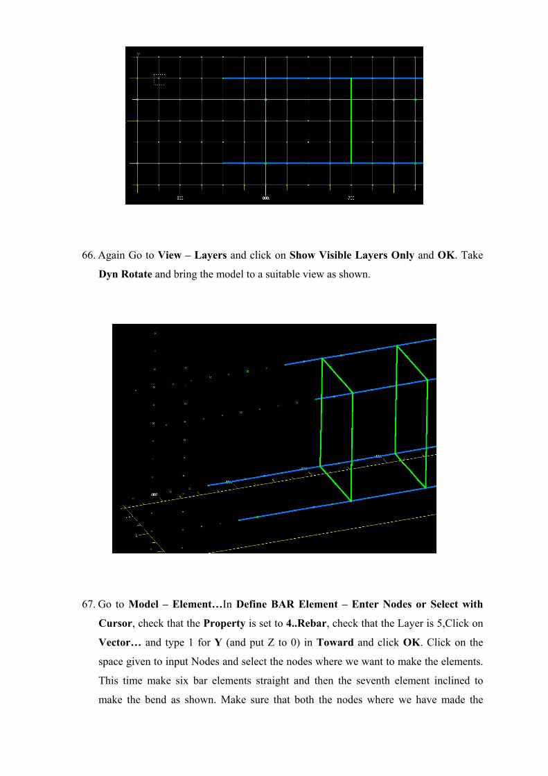
66. Again Go to View – Layers and click on Show Visible Layers Only and OK. Take
Dyn Rotate and bring the model to a suitable view as shown.
67. Go to Model – Element…In Define BAR Element – Enter Nodes or Select with
Cursor, check that the Property is set to 4..Rebar, check that the Layer is 5,Click on
Vector… and type 1 for Y (and put Z to 0) in Toward and click OK. Click on the
space given to input Nodes and select the nodes where we want to make the elements.
This time make six bar elements straight and then the seventh element inclined to
make the bend as shown. Make sure that both the nodes where we have made the
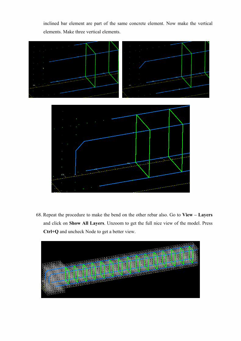
inclined bar element are part of the same concrete element. Now make the vertical
elements. Make three vertical elements.
68. Repeat the procedure to make the bend on the other rebar also. Go to View – Layers
and click on Show All Layers. Unzoom to get the full nice view of the model. Press
Ctrl+Q and uncheck Node to get a better view.
69. Go to Tools – Check – Coincident Nodes… Under Entity Selection - Select Node(s)
to Check, Click on Select All. Click OK. In the Check/Merge Coincident dialog
box, check the Merge Coincident Entities check box. Click OK.
70. Before proceeding further, let us make the model to half model so that we can use
symmetry and reduce the number of elements. Although in this case the number of
elements is not very large because we used very coarse mesh size but when we use
finer mesh, half model helps in saving significant time. Press F8 and take YZ Right
view. Click OK and zoom in to get better view.
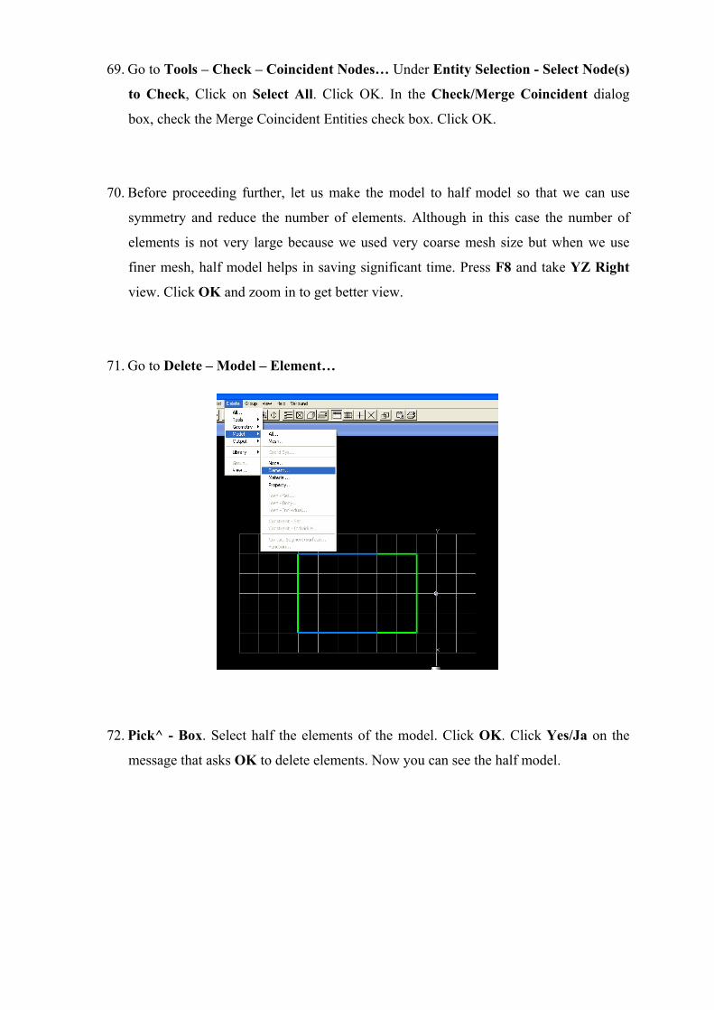
71. Go to Delete – Model – Element…
72. Pick^ - Box. Select half the elements of the model. Click OK. Click Yes/Ja on the
message that asks OK to delete elements. Now you can see the half model.
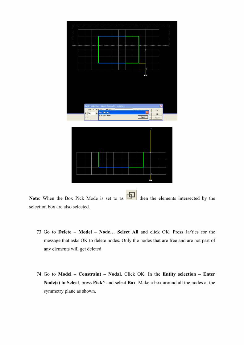
Note: When the Box Pick Mode is set to as then the elements intersected by the
selection box are also selected.
73. Go to Delete – Model – Node… Select All and click OK. Press Ja/Yes for the
message that asks OK to delete nodes. Only the nodes that are free and are not part of
any elements will get deleted.
74. Go to Model – Constraint – Nodal. Click OK. In the Entity selection – Enter
Node(s) to Select, press Pick^ and select Box. Make a box around all the nodes at the
symmetry plane as shown.
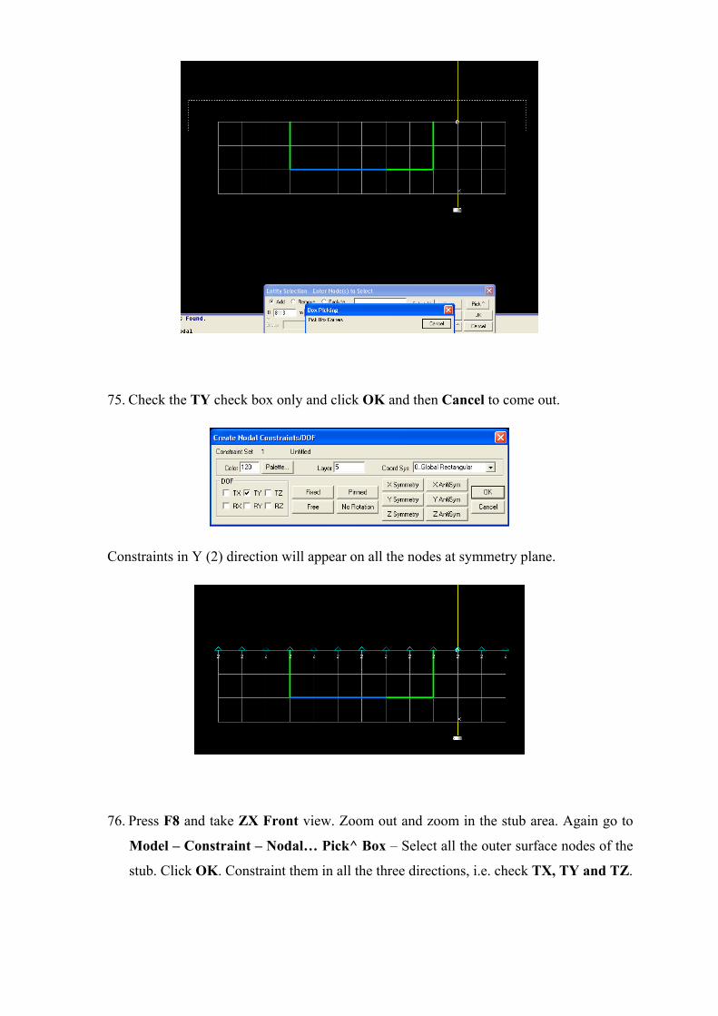
75. Check the TY check box only and click OK and then Cancel to come out.
Constraints in Y (2) direction will appear on all the nodes at symmetry plane.
76. Press F8 and take ZX Front view. Zoom out and zoom in the stub area. Again go to
Model – Constraint – Nodal… Pick^ Box – Select all the outer surface nodes of the
stub. Click OK. Constraint them in all the three directions, i.e. check TX, TY and TZ.
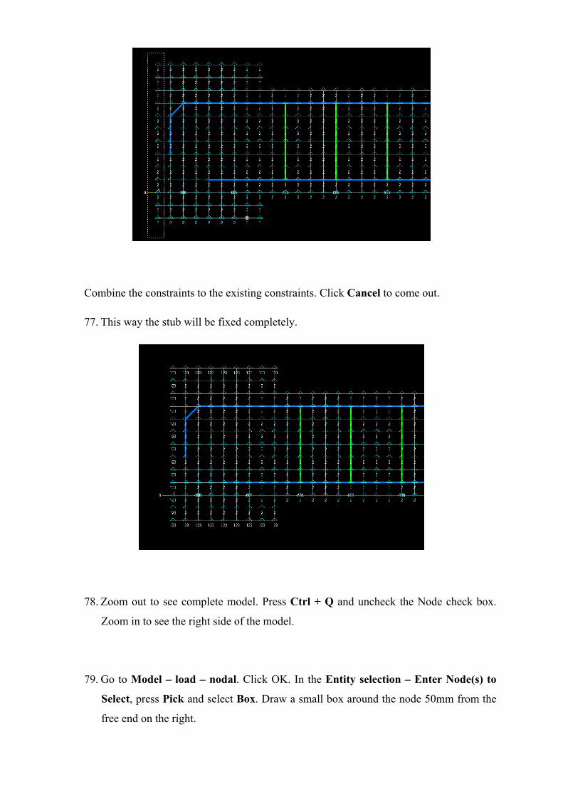
Combine the constraints to the existing constraints. Click Cancel to come out.
77. This way the stub will be fixed completely.
78. Zoom out to see complete model. Press Ctrl + Q and uncheck the Node check box.
Zoom in to see the right side of the model.
79. Go to Model – load – nodal. Click OK. In the Entity selection – Enter Node(s) to
Select, press Pick and select Box. Draw a small box around the node 50mm from the
free end on the right.
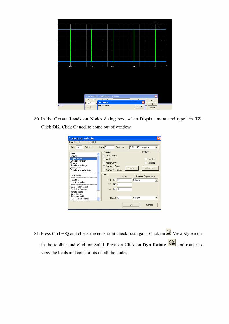
80. In the Create Loads on Nodes dialog box, select Displacement and type 1in TZ.
Click OK. Click Cancel to come out of window.
81. Press Ctrl + Q and check the constraint check box again. Click on View style icon
in the toolbar and click on Solid. Press on Click on Dyn Rotate and rotate to
view the loads and constraints on all the nodes.
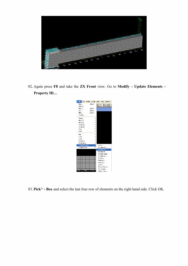
82. Again press F8 and take the ZX Front view. Go to Modify – Update Elements –
Property ID…
83. Pick^ - Box and select the last four row of elements on the right hand side. Click OK.
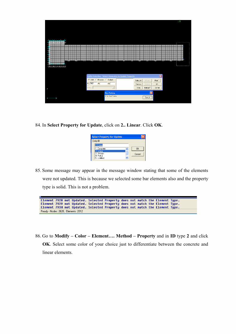
84. In Select Property for Update, click on 2.. Linear. Click OK.
85. Some message may appear in the message window stating that some of the elements
were not updated. This is because we selected some bar elements also and the property
type is solid. This is not a problem.
86. Go to Modify – Color – Element…. Method – Property and in ID type 2 and click
OK. Select some color of your choice just to differentiate between the concrete and
linear elements.
87. Go to Delete – Model – Property. In the Entity Selection – Select Property(s) to
Delete dialog box, click on Select All and click OK.
88. Go to Modify – Renumber – Element… Select All and click OK. In the Renumber
To Dialog box, Click on X. Starting ID should be 1 and Increment should also be 1.
Click OK.
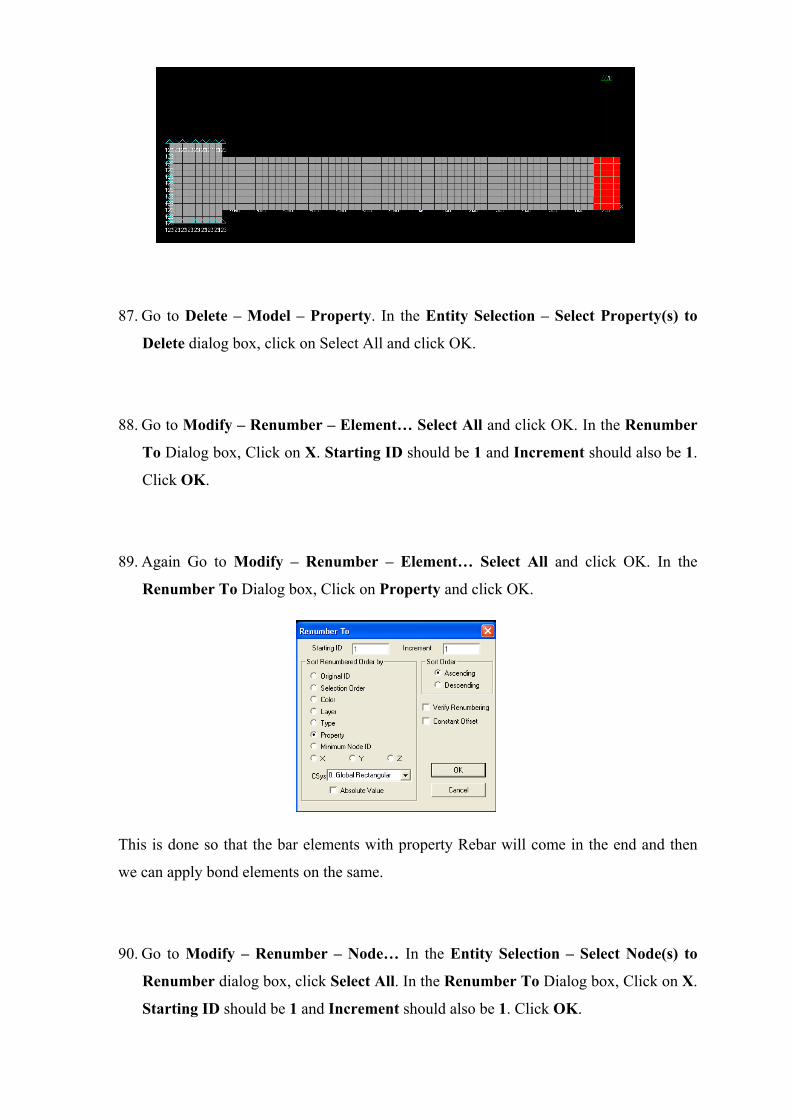
89. Again Go to Modify – Renumber – Element… Select All and click OK. In the
Renumber To Dialog box, Click on Property and click OK.
This is done so that the bar elements with property Rebar will come in the end and then
we can apply bond elements on the same.
90. Go to Modify – Renumber – Node… In the Entity Selection – Select Node(s) to
Renumber dialog box, click Select All. In the Renumber To Dialog box, Click on X.
Starting ID should be 1 and Increment should also be 1. Click OK.
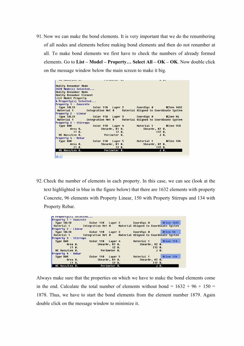
91. Now we can make the bond elements. It is very important that we do the renumbering
of all nodes and elements before making bond elements and then do not renumber at
all. To make bond elements we first have to check the numbers of already formed
elements. Go to List – Model – Property… Select All – OK – OK. Now double click
on the message window below the main screen to make it big.
92. Check the number of elements in each property. In this case, we can see (look at the
text highlighted in blue in the figure below) that there are 1632 elements with property
Concrete, 96 elements with Property Linear, 150 with Property Stirrups and 134 with
Property Rebar.
Always make sure that the properties on which we have to make the bond elements come
in the end. Calculate the total number of elements without bond = 1632 + 96 + 150 =
1878. Thus, we have to start the bond elements from the element number 1879. Again
double click on the message window to minimize it.
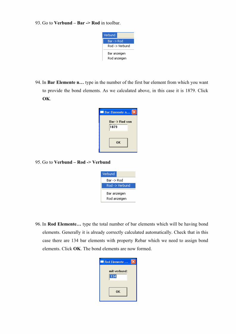
93. Go to Verbund – Bar -> Rod in toolbar.
94. In Bar Elemente n… type in the number of the first bar element from which you want
to provide the bond elements. As we calculated above, in this case it is 1879. Click
OK.
95. Go to Verbund – Rod -> Verbund
96. In Rod Elemente… type the total number of bar elements which will be having bond
elements. Generally it is already correctly calculated automatically. Check that in this
case there are 134 bar elements with property Rebar which we need to assign bond
elements. Click OK. The bond elements are now formed.
97. To check whether bond elements are formed, take wireframe view and zoom in near
the Rebar. Go to View – Show – Node – OK. Click on any node to which Rebar
element is connected. You may notice that at same location you can select 2 nodes.
One node (the one with smaller number) is the part of solid element and the other node
(one with larger number) is connected to rebar. And they both are connected with a
zero length 1D Bond element.
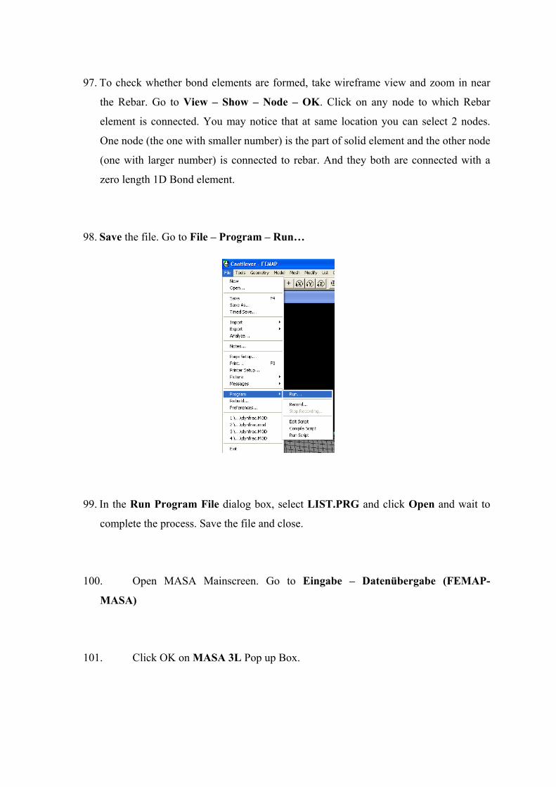
98. Save the file. Go to File – Program – Run…
99. In the Run Program File dialog box, select LIST.PRG and click Open and wait to
complete the process. Save the file and close.
100. Open MASA Mainscreen. Go to Eingabe – Datenübergabe (FEMAP-
MASA)
101. Click OK on MASA 3L Pop up Box.
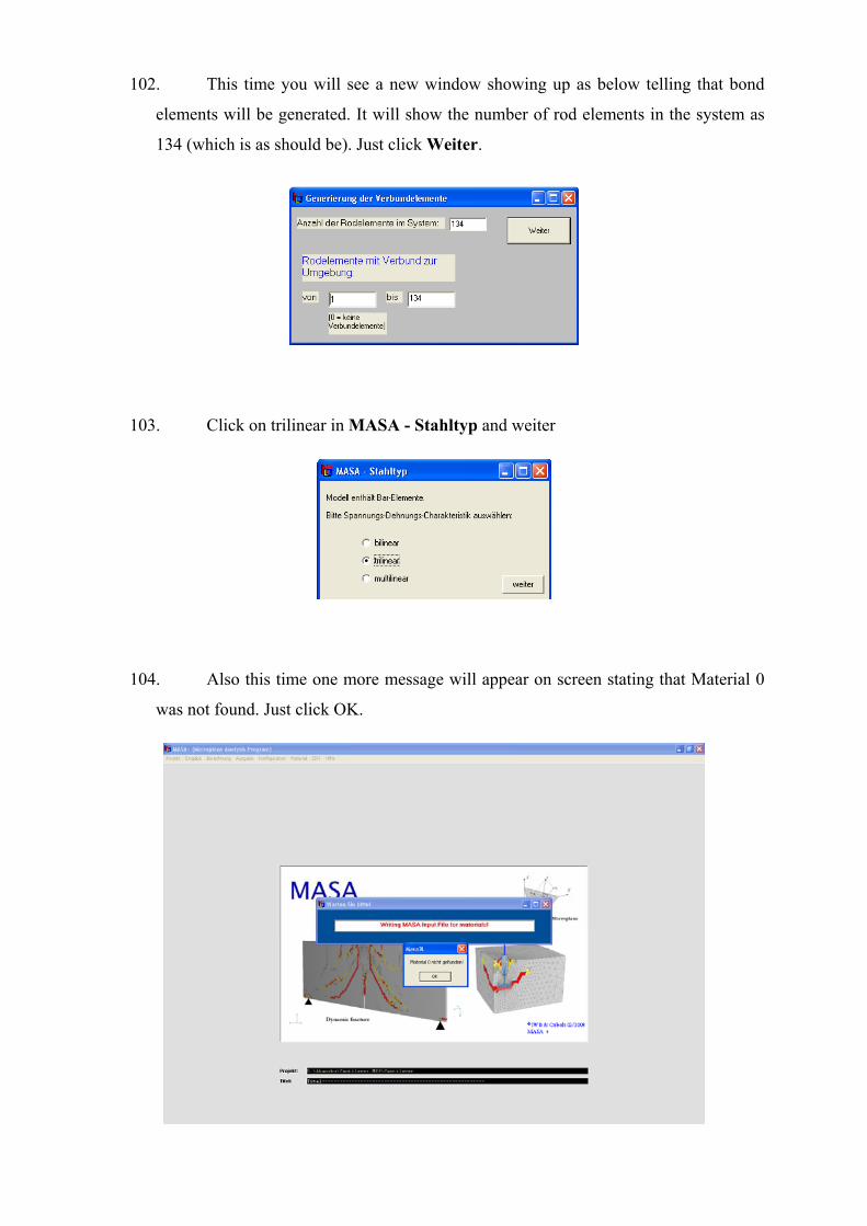
102. This time you will see a new window showing up as below telling that bond
elements will be generated. It will show the number of rod elements in the system as
134 (which is as should be). Just click Weiter.
103. Click on trilinear in MASA - Stahltyp and weiter
104. Also this time one more message will appear on screen stating that Material 0
was not found. Just click OK.
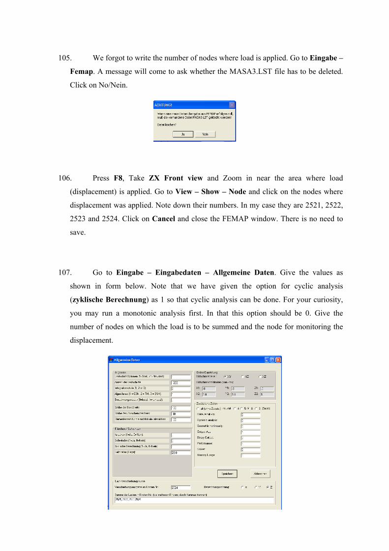
105. We forgot to write the number of nodes where load is applied. Go to Eingabe –
Femap. A message will come to ask whether the MASA3.LST file has to be deleted.
Click on No/Nein.
106. Press F8, Take ZX Front view and Zoom in near the area where load
(displacement) is applied. Go to View – Show – Node and click on the nodes where
displacement was applied. Note down their numbers. In my case they are 2521, 2522,
2523 and 2524. Click on Cancel and close the FEMAP window. There is no need to
save.
107. Go to Eingabe – Eingabedaten – Allgemeine Daten. Give the values as
shown in form below. Note that we have given the option for cyclic analysis
(zyklische Berechnung) as 1 so that cyclic analysis can be done. For your curiosity,
you may run a monotonic analysis first. In that this option should be 0. Give the
number of nodes on which the load is to be summed and the node for monitoring the
displacement.
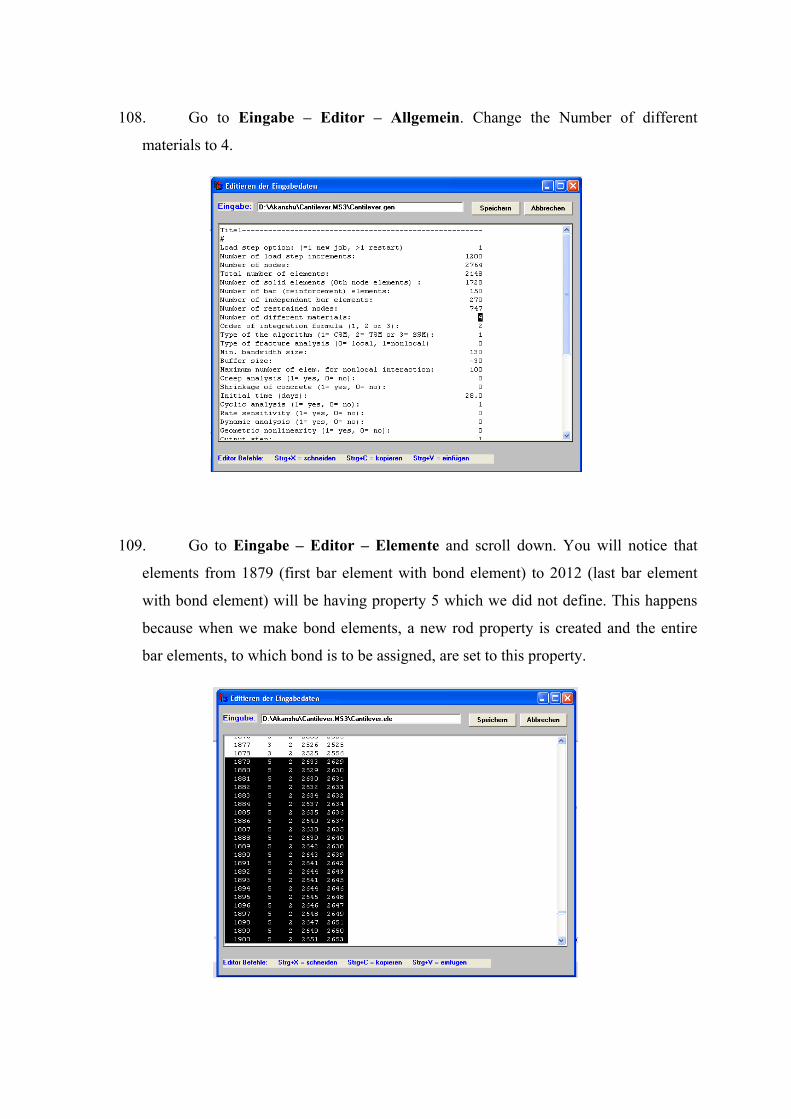
108. Go to Eingabe – Editor – Allgemein. Change the Number of different
materials to 4.
109. Go to Eingabe – Editor – Elemente and scroll down. You will notice that
elements from 1879 (first bar element with bond element) to 2012 (last bar element
with bond element) will be having property 5 which we did not define. This happens
because when we make bond elements, a new rod property is created and the entire
bar elements, to which bond is to be assigned, are set to this property.
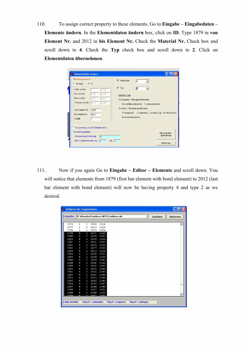
110. To assign correct property to these elements, Go to Eingabe – Eingabedaten –
Elemente ändern. In the Elementdaten ändern box, click on ID. Type 1879 in von
Element Nr. and 2012 in bis Element Nr. Check the Material Nr. Check box and
scroll down to 4. Check the Typ check box and scroll down to 2. Click on
Elementdaten übernehmen.
111. Now if you again Go to Eingabe – Editor – Elemente and scroll down. You
will notice that elements from 1879 (first bar element with bond element) to 2012 (last
bar element with bond element) will now be having property 4 and type 2 as we
desired.
112. Again Go to Eingabe – Eingabedaten – Elemente ändern. In the
Elementdaten ändern form, select Material Nr. 2 from the drop down. Check Typ
check box and select 1 from dropdown for linearelastich. Click on Elementdaten
übernehmen. This is done to make the elements with property 2 (steel plate) have
linear elastic properties.
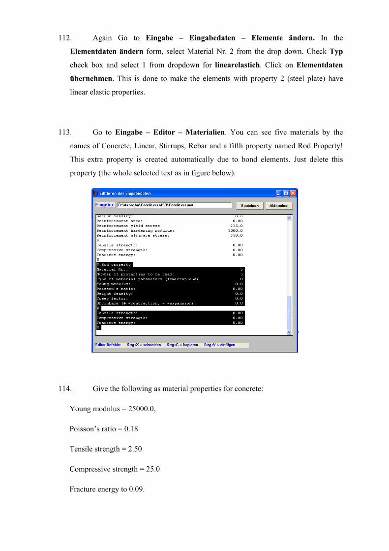
113. Go to Eingabe – Editor – Materialien. You can see five materials by the
names of Concrete, Linear, Stirrups, Rebar and a fifth property named Rod Property!
This extra property is created automatically due to bond elements. Just delete this
property (the whole selected text as in figure below).
114. Give the following as material properties for concrete:
Young modulus = 25000.0,
Poisson’s ratio = 0.18
Tensile strength = 2.50
Compressive strength = 25.0
Fracture energy to 0.09.
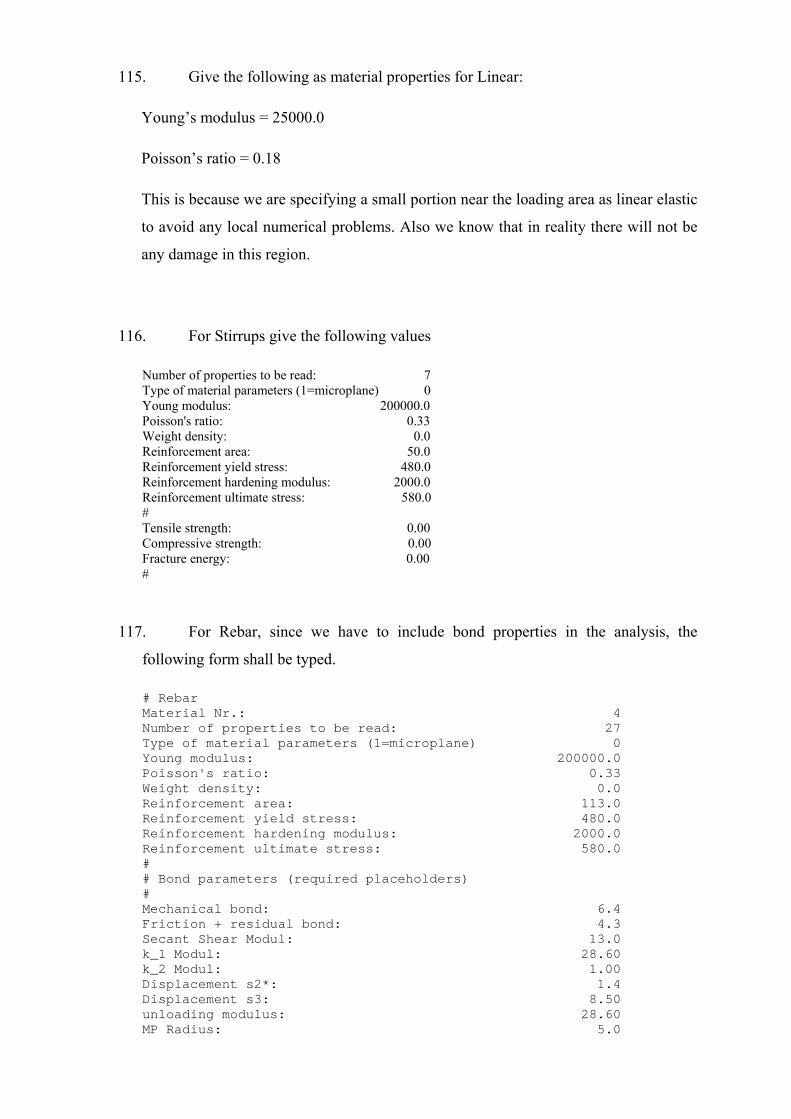
115. Give the following as material properties for Linear:
Young’s modulus = 25000.0
Poisson’s ratio = 0.18
This is because we are specifying a small portion near the loading area as linear elastic
to avoid any local numerical problems. Also we know that in reality there will not be
any damage in this region.
116. For Stirrups give the following values
Number of properties to be read: 7 Type of material parameters (1=microplane) 0 Young modulus: 200000.0 Poisson's ratio: 0.33 Weight density: 0.0 Reinforcement area: 50.0 Reinforcement yield stress: 480.0 Reinforcement hardening modulus: 2000.0 Reinforcement ultimate stress: 580.0 # Tensile strength: 0.00 Compressive strength: 0.00 Fracture energy: 0.00 #
117. For Rebar, since we have to include bond properties in the analysis, the
following form shall be typed.
# Rebar Material Nr.: 4 Number of properties to be read: 27 Type of material parameters (1=microplane) 0 Young modulus: 200000.0 Poisson's ratio: 0.33 Weight density: 0.0 Reinforcement area: 113.0 Reinforcement yield stress: 480.0 Reinforcement hardening modulus: 2000.0 Reinforcement ultimate stress: 580.0 # # Bond parameters (required placeholders) # Mechanical bond: 6.4 Friction + residual bond: 4.3 Secant Shear Modul: 13.0 k_1 Modul: 28.60 k_2 Modul: 1.00 Displacement s2*: 1.4 Displacement s3: 8.50 unloading modulus: 28.60 MP Radius: 5.0
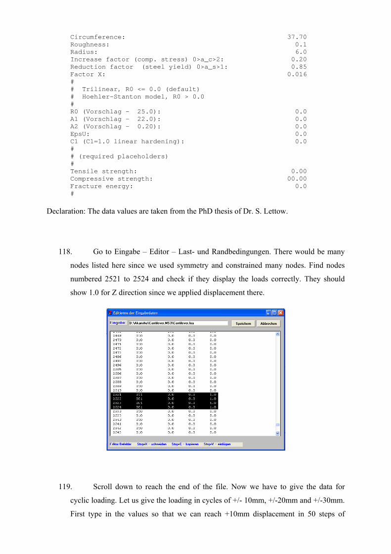
Circumference: 37.70 Roughness: 0.1 Radius: 6.0 Increase factor (comp. stress) 0>a_c>2: 0.20 Reduction factor (steel yield) 0>a_s>1: 0.85 Factor X: 0.016 # # Trilinear, R0 <= 0.0 (default) # Hoehler-Stanton model, R0 > 0.0 # R0 (Vorschlag - 25.0): 0.0 A1 (Vorschlag - 22.0): 0.0 A2 (Vorschlag - 0.20): 0.0 EpsU: 0.0 C1 (C1=1.0 linear hardening): 0.0 # # (required placeholders) # Tensile strength: 0.00 Compressive strength: 00.00 Fracture energy: 0.0 #
Declaration: The data values are taken from the PhD thesis of Dr. S. Lettow.
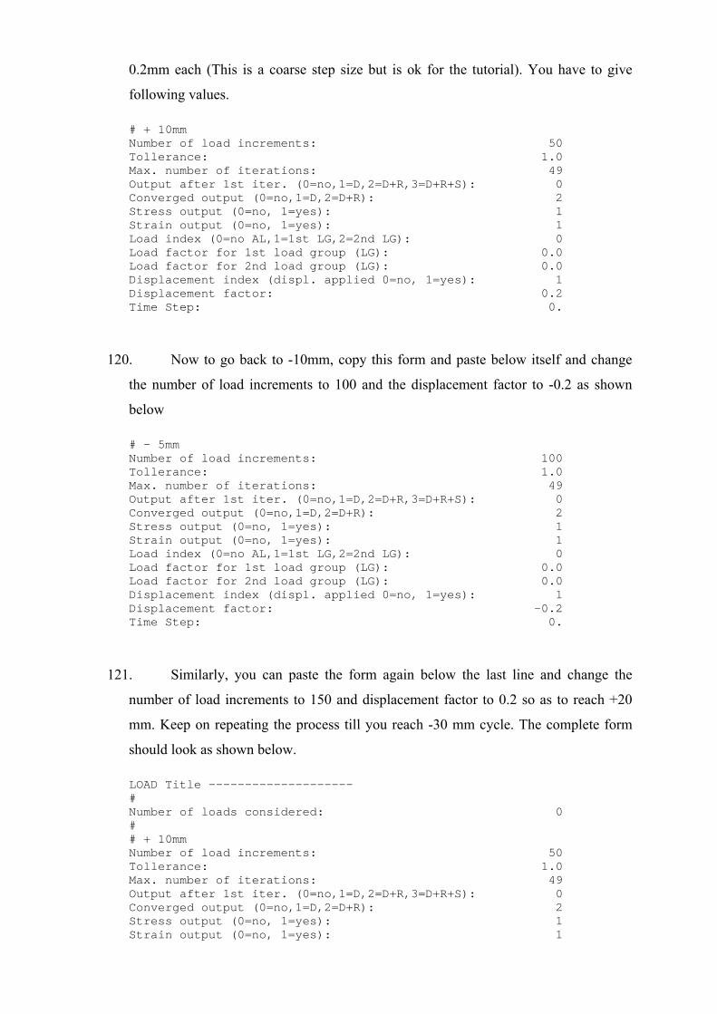
118. Go to Eingabe – Editor – Last- und Randbedingungen. There would be many
nodes listed here since we used symmetry and constrained many nodes. Find nodes
numbered 2521 to 2524 and check if they display the loads correctly. They should
show 1.0 for Z direction since we applied displacement there.
119. Scroll down to reach the end of the file. Now we have to give the data for
cyclic loading. Let us give the loading in cycles of +/- 10mm, +/-20mm and +/-30mm.
First type in the values so that we can reach +10mm displacement in 50 steps of
0.2mm each (This is a coarse step size but is ok for the tutorial). You have to give
following values.
# + 10mm Number of load increments: 50 Tollerance: 1.0 Max. number of iterations: 49 Output after 1st iter. (0=no,1=D,2=D+R,3=D+R+S): 0 Converged output (0=no,1=D,2=D+R): 2 Stress output (0=no, 1=yes): 1 Strain output (0=no, 1=yes): 1 Load index (0=no AL,1=1st LG,2=2nd LG): 0 Load factor for 1st load group (LG): 0.0 Load factor for 2nd load group (LG): 0.0 Displacement index (displ. applied 0=no, 1=yes): 1 Displacement factor: 0.2 Time Step: 0.
120. Now to go back to -10mm, copy this form and paste below itself and change
the number of load increments to 100 and the displacement factor to -0.2 as shown
below
# - 5mm Number of load increments: 100 Tollerance: 1.0 Max. number of iterations: 49 Output after 1st iter. (0=no,1=D,2=D+R,3=D+R+S): 0 Converged output (0=no,1=D,2=D+R): 2 Stress output (0=no, 1=yes): 1 Strain output (0=no, 1=yes): 1 Load index (0=no AL,1=1st LG,2=2nd LG): 0 Load factor for 1st load group (LG): 0.0 Load factor for 2nd load group (LG): 0.0 Displacement index (displ. applied 0=no, 1=yes): 1 Displacement factor: -0.2 Time Step: 0.
121. Similarly, you can paste the form again below the last line and change the
number of load increments to 150 and displacement factor to 0.2 so as to reach +20
mm. Keep on repeating the process till you reach -30 mm cycle. The complete form
should look as shown below.
LOAD Title -------------------- # Number of loads considered: 0 # # + 10mm Number of load increments: 50 Tollerance: 1.0 Max. number of iterations: 49 Output after 1st iter. (0=no,1=D,2=D+R,3=D+R+S): 0 Converged output (0=no,1=D,2=D+R): 2 Stress output (0=no, 1=yes): 1 Strain output (0=no, 1=yes): 1
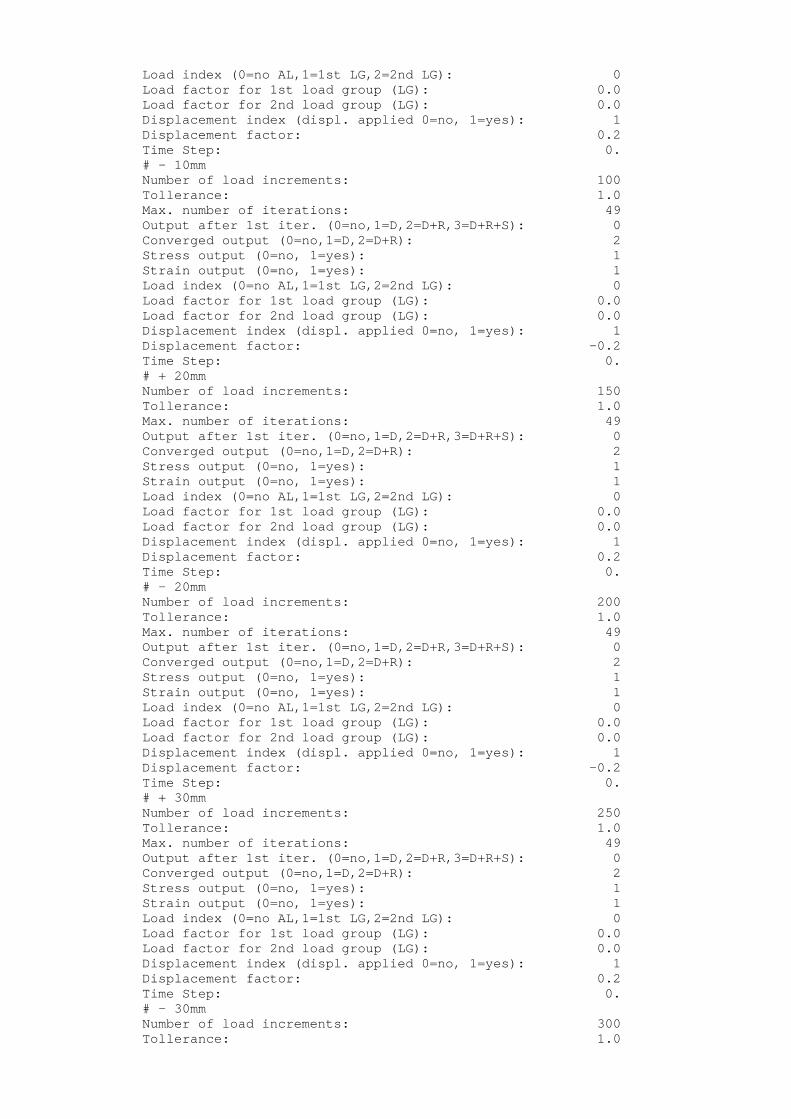
Load index (0=no AL,1=1st LG,2=2nd LG): 0 Load factor for 1st load group (LG): 0.0 Load factor for 2nd load group (LG): 0.0 Displacement index (displ. applied 0=no, 1=yes): 1 Displacement factor: 0.2 Time Step: 0. # - 10mm Number of load increments: 100 Tollerance: 1.0 Max. number of iterations: 49 Output after 1st iter. (0=no,1=D,2=D+R,3=D+R+S): 0 Converged output (0=no,1=D,2=D+R): 2 Stress output (0=no, 1=yes): 1 Strain output (0=no, 1=yes): 1 Load index (0=no AL,1=1st LG,2=2nd LG): 0 Load factor for 1st load group (LG): 0.0 Load factor for 2nd load group (LG): 0.0 Displacement index (displ. applied 0=no, 1=yes): 1 Displacement factor: -0.2 Time Step: 0. # + 20mm Number of load increments: 150 Tollerance: 1.0 Max. number of iterations: 49 Output after 1st iter. (0=no,1=D,2=D+R,3=D+R+S): 0 Converged output (0=no,1=D,2=D+R): 2 Stress output (0=no, 1=yes): 1 Strain output (0=no, 1=yes): 1 Load index (0=no AL,1=1st LG,2=2nd LG): 0 Load factor for 1st load group (LG): 0.0 Load factor for 2nd load group (LG): 0.0 Displacement index (displ. applied 0=no, 1=yes): 1 Displacement factor: 0.2 Time Step: 0. # - 20mm Number of load increments: 200 Tollerance: 1.0 Max. number of iterations: 49 Output after 1st iter. (0=no,1=D,2=D+R,3=D+R+S): 0 Converged output (0=no,1=D,2=D+R): 2 Stress output (0=no, 1=yes): 1 Strain output (0=no, 1=yes): 1 Load index (0=no AL,1=1st LG,2=2nd LG): 0 Load factor for 1st load group (LG): 0.0 Load factor for 2nd load group (LG): 0.0 Displacement index (displ. applied 0=no, 1=yes): 1 Displacement factor: -0.2 Time Step: 0. # + 30mm Number of load increments: 250 Tollerance: 1.0 Max. number of iterations: 49 Output after 1st iter. (0=no,1=D,2=D+R,3=D+R+S): 0 Converged output (0=no,1=D,2=D+R): 2 Stress output (0=no, 1=yes): 1 Strain output (0=no, 1=yes): 1 Load index (0=no AL,1=1st LG,2=2nd LG): 0 Load factor for 1st load group (LG): 0.0 Load factor for 2nd load group (LG): 0.0 Displacement index (displ. applied 0=no, 1=yes): 1 Displacement factor: 0.2 Time Step: 0. # - 30mm Number of load increments: 300 Tollerance: 1.0
Max. number of iterations: 49 Output after 1st iter. (0=no,1=D,2=D+R,3=D+R+S): 0 Converged output (0=no,1=D,2=D+R): 2 Stress output (0=no, 1=yes): 1 Strain output (0=no, 1=yes): 1 Load index (0=no AL,1=1st LG,2=2nd LG): 0 Load factor for 1st load group (LG): 0.0 Load factor for 2nd load group (LG): 0.0 Displacement index (displ. applied 0=no, 1=yes): 1 Displacement factor: 0.2 Time Step: 0. # 0mm Number of load increments: 150 Tollerance: 1.0 Max. number of iterations: 49 Output after 1st iter. (0=no,1=D,2=D+R,3=D+R+S): 0 Converged output (0=no,1=D,2=D+R): 2 Stress output (0=no, 1=yes): 1 Strain output (0=no, 1=yes): 1 Load index (0=no AL,1=1st LG,2=2nd LG): 0 Load factor for 1st load group (LG): 0.0 Load factor for 2nd load group (LG): 0.0 Displacement index (displ. applied 0=no, 1=yes): 1 Displacement factor: 0.2 Time Step: 0. #
Note that the sum total of number of load increments comes to 1200 and that is what we
gave in allgemein file too.
122. Now you are finished with all the required inputs. Click Berechnung. A
Fortran window showing the status of calculations will appear. This time you may
have to wait for long since the number of steps is very large, but it is worth it, have
patience.
123. However, you may not have to wait till the completion of the analysis to view
the progress. Even while the program is running, you may click on Ausgabe – Last-
Verschiebung to See the Load-Displacement curve. Also at any time you may go to
Ausgabe – Post Utility, select a few results and then to Ausgabe – FEMAP to view
the results. This is same as was explained in previous tutorial. Here we will only
discuss the results after completion.
124. After the analysis is complete, press Enter to close the fortran window. To See
the Load-Displacement curve, go to Ausgabe – Last-Verschiebung.
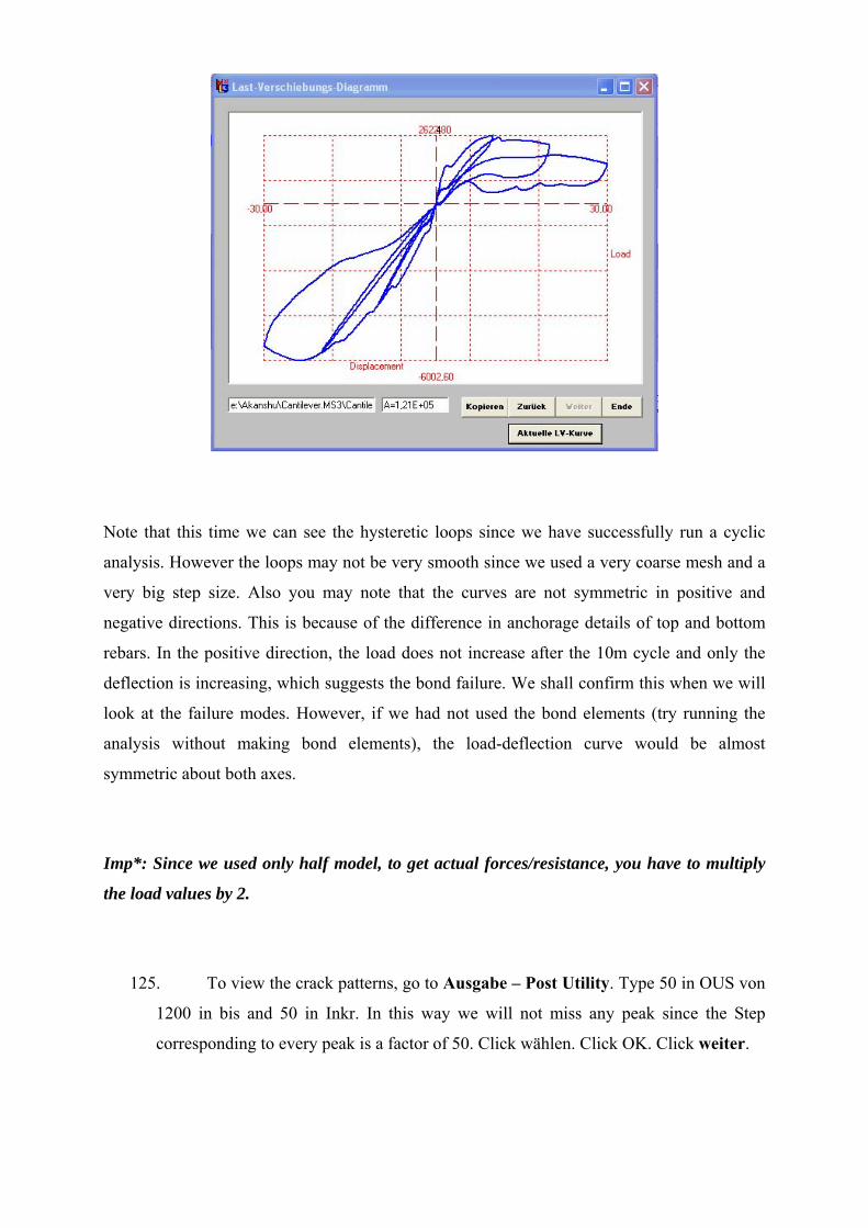
Note that this time we can see the hysteretic loops since we have successfully run a cyclic
analysis. However the loops may not be very smooth since we used a very coarse mesh and a
very big step size. Also you may note that the curves are not symmetric in positive and
negative directions. This is because of the difference in anchorage details of top and bottom
rebars. In the positive direction, the load does not increase after the 10m cycle and only the
deflection is increasing, which suggests the bond failure. We shall confirm this when we will
look at the failure modes. However, if we had not used the bond elements (try running the
analysis without making bond elements), the load-deflection curve would be almost
symmetric about both axes.
Imp*: Since we used only half model, to get actual forces/resistance, you have to multiply
the load values by 2.
125. To view the crack patterns, go to Ausgabe – Post Utility. Type 50 in OUS von
1200 in bis and 50 in Inkr. In this way we will not miss any peak since the Step
corresponding to every peak is a factor of 50. Click wählen. Click OK. Click weiter.
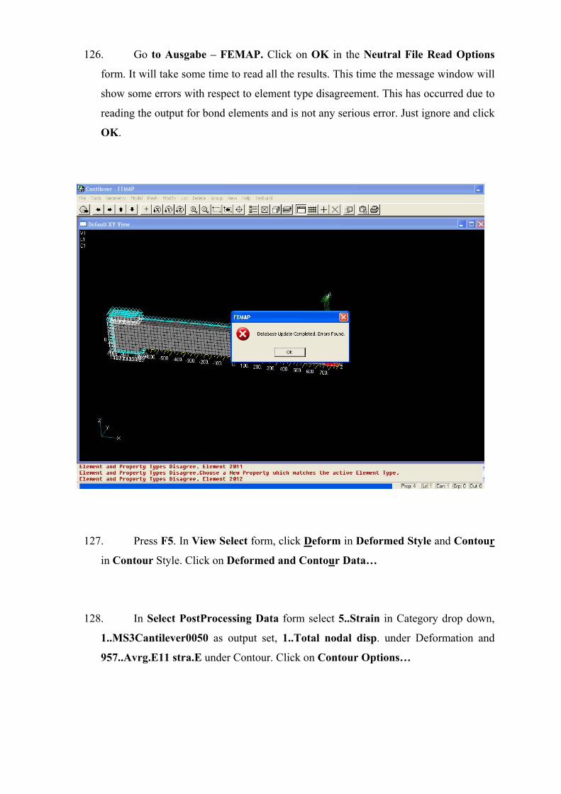
126. Go to Ausgabe – FEMAP. Click on OK in the Neutral File Read Options
form. It will take some time to read all the results. This time the message window will
show some errors with respect to element type disagreement. This has occurred due to
reading the output for bond elements and is not any serious error. Just ignore and click
OK.
127. Press F5. In View Select form, click Deform in Deformed Style and Contour
in Contour Style. Click on Deformed and Contour Data…
128. In Select PostProcessing Data form select 5..Strain in Category drop down,
1..MS3Cantilever0050 as output set, 1..Total nodal disp. under Deformation and
957..Avrg.E11 stra.E under Contour. Click on Contour Options…
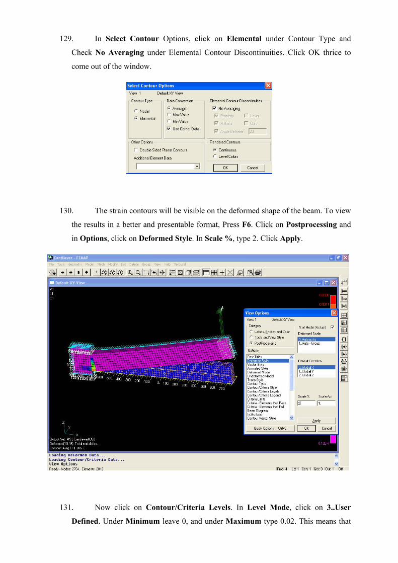
129. In Select Contour Options, click on Elemental under Contour Type and
Check No Averaging under Elemental Contour Discontinuities. Click OK thrice to
come out of the window.
130. The strain contours will be visible on the deformed shape of the beam. To view
the results in a better and presentable format, Press F6. Click on Postprocessing and
in Options, click on Deformed Style. In Scale %, type 2. Click Apply.
131. Now click on Contour/Criteria Levels. In Level Mode, click on 3..User
Defined. Under Minimum leave 0, and under Maximum type 0.02. This means that
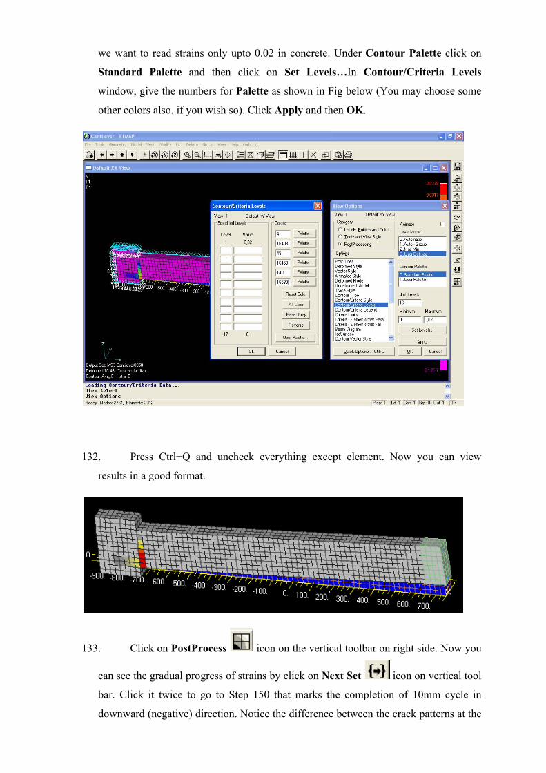
we want to read strains only upto 0.02 in concrete. Under Contour Palette click on
Standard Palette and then click on Set Levels…In Contour/Criteria Levels
window, give the numbers for Palette as shown in Fig below (You may choose some
other colors also, if you wish so). Click Apply and then OK.
132. Press Ctrl+Q and uncheck everything except element. Now you can view
results in a good format.
133. Click on PostProcess icon on the vertical toolbar on right side. Now you
can see the gradual progress of strains by click on Next Set icon on vertical tool
bar. Click it twice to go to Step 150 that marks the completion of 10mm cycle in
downward (negative) direction. Notice the difference between the crack patterns at the
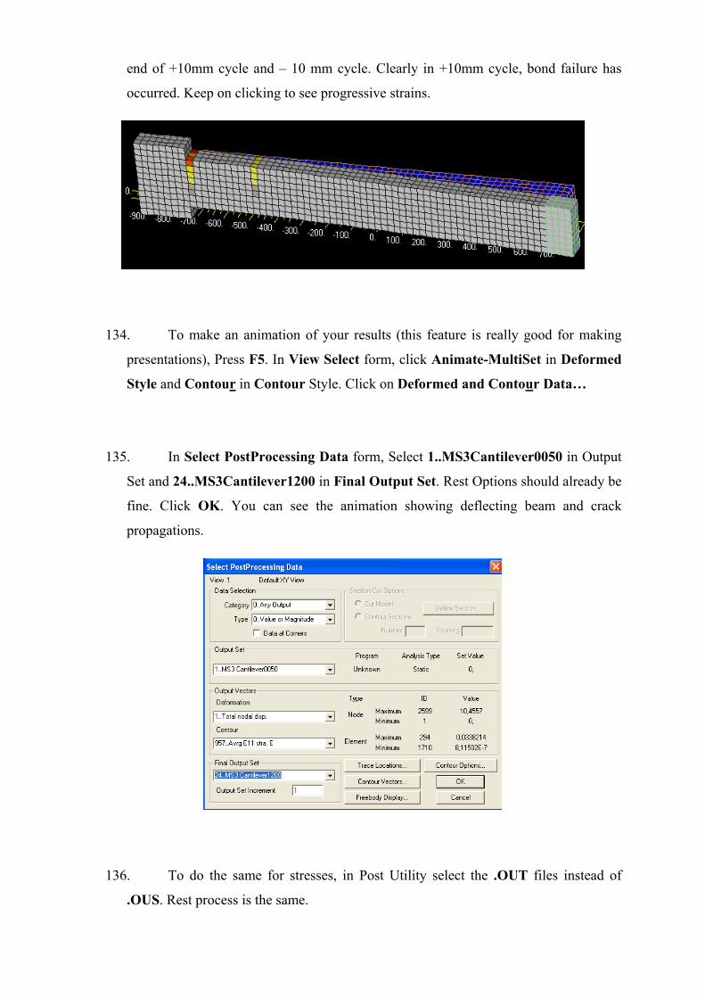
end of +10mm cycle and – 10 mm cycle. Clearly in +10mm cycle, bond failure has
occurred. Keep on clicking to see progressive strains.
134. To make an animation of your results (this feature is really good for making
presentations), Press F5. In View Select form, click Animate-MultiSet in Deformed
Style and Contour in Contour Style. Click on Deformed and Contour Data…
135. In Select PostProcessing Data form, Select 1..MS3Cantilever0050 in Output
Set and 24..MS3Cantilever1200 in Final Output Set. Rest Options should already be
fine. Click OK. You can see the animation showing deflecting beam and crack
propagations.
136. To do the same for stresses, in Post Utility select the .OUT files instead of
.OUS. Rest process is the same.

HAVE A GREAT TIME AHEAD WITH MASA AND FEMAP.


![Full MASA FEMAP Tutorial for RC Structural Elements Rev-April2012[1]](https://static.fdocuments.us/doc/165x107/55cf8cc25503462b138f919d/full-masa-femap-tutorial-for-rc-structural-elements-rev-april20121.jpg)