A beginner’s guide to SSA(Singular Spectrum Analysis)by David Claessen (CERES-ERTI) and Andreas Groth (LMD)CERES-ERTI, Ecole Normale Supérieure, Paris, www.environnement.ens.fr

This guide is intended as a down-to-earth introduction to SSA using a very simple example. The idea is to do the calculations step by step, using a short time series. The different key words and key concepts should become clear through this stepwise computation. This is, however, in no way a rigorous mathematical introduction to SSA. For a rigorous and advanced introduction, please refer to the review paper Ghil et al. (2002) “Advanced spectral methods for climatic time series”, Rev Geophys 40(1): 3.1–3.41. We use the software Scilab, a free alternative to Matlab, as well as the SSA-MTM Toolkit, an equally free software package, specifically designed for doing SSA and other spectral analysis methods. A comprehensive (and advanced) user guide of the SSA-MTM Toolkit, written by the SSA-MTM Group at UCLA, is available online here: www.atmos.ucla.edu/tcd/ssa/

The idea of SSA is to decompose a time series into oscillatory components and noise; we hope to catch a glimpse (or better, to characterize) the underlying regular dynamical behavior which is the signature of the dynamical system under study. The method relies on elementary linear algebra: a basic understanding of concepts such as matrix-vector products, eigenvalues and eigenvectors is hence necessary.

1. SSA page 21. How to compute EOFs and their eigenvalues page 22. Principal components page 63. Reconstruction page 74. How to interpret SSA analysis page 10

2. MSSA page 111. How to compute EOFs and their eigenvalues page 112. Principal components page 133. Reconstruction page 144. Advantages of MSSA with respect to SSA page 165. Tips for MSSA with the SSA-MTM toolkit page 16

3. Glossary page 17

4. References page 17

5. Appendix: Scilab scripts page 17

1

1. Singular Spectral Analysis – Univariate caseFirst of all we consider the univariate case. That means a single time series is given. Later on we will generalize to the multivariate case.

1.1 How to compute EOFs and their eigenvalues

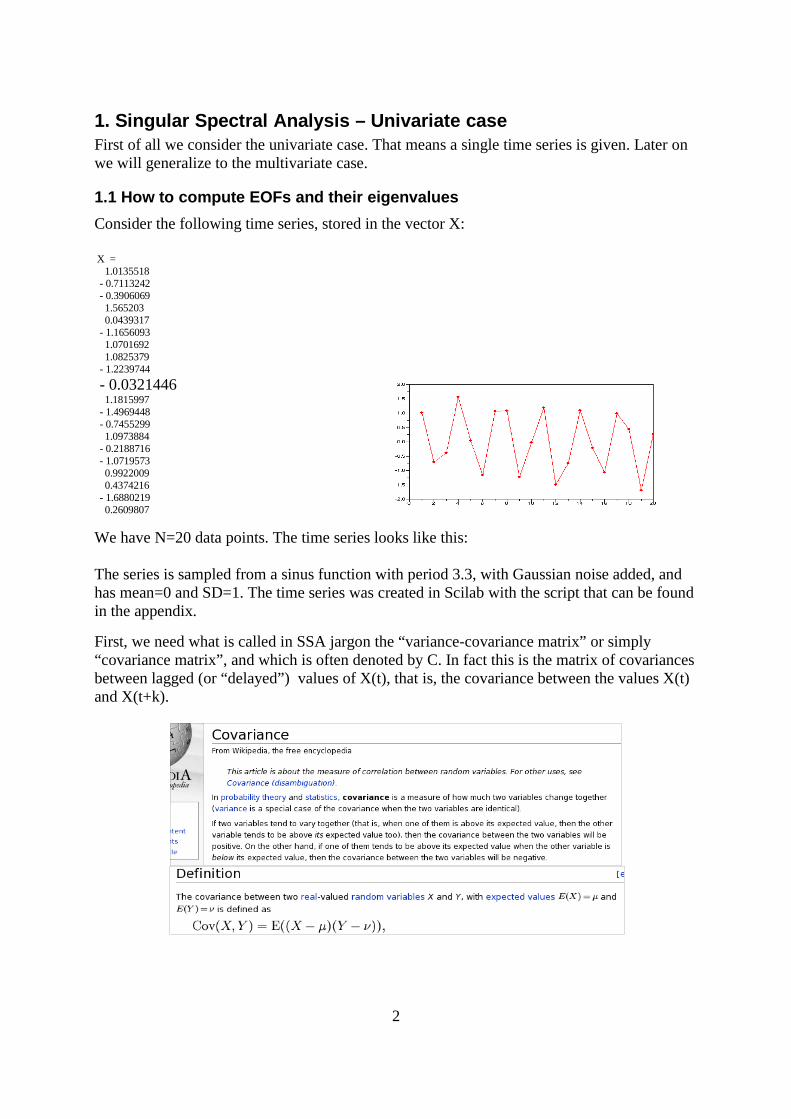
Consider the following time series, stored in the vector X:

X = 1.0135518 - 0.7113242 - 0.3906069 1.565203 0.0439317 - 1.1656093 1.0701692 1.0825379 - 1.2239744

- 0.0321446 1.1815997 - 1.4969448 - 0.7455299 1.0973884 - 0.2188716 - 1.0719573 0.9922009 0.4374216 - 1.6880219 0.2609807

We have N=20 data points. The time series looks like this:

The series is sampled from a sinus function with period 3.3, with Gaussian noise added, and has mean=0 and SD=1. The time series was created in Scilab with the script that can be found in the appendix.

First, we need what is called in SSA jargon the “variance-covariance matrix” or simply “covariance matrix”, and which is often denoted by C. In fact this is the matrix of covariances between lagged (or “delayed”) values of X(t), that is, the covariance between the values X(t) and X(t+k).

2

The idea is thus to compute the covariance between the values X(t) and X(t+k), where k is a delay (or “lag”). That is, using the definition above, if the covariance at lag k is positive, the values X(t) and X(t+k) tend to vary together. For example, guessing from the figure above, is seems that the covariance is positive at lag k=3, and negative for k=1 or k=2.

Here we show two different ways to compute C.

First method to compute C. We compute the covariances between the values X(t) and X(t+k) by using the Scilab built-in function “corr” (NB in engineering covariance is referred to as correlation, hence the function name “corr”. In Matlab the same function is called “cov”). Giving the statement covX=corr(X,M) gives us the vector covX of size M. If we choose “window size” M=4, i.e., we only consider lags of k=0,1,2 and 3, then

covX = 1. - 0.2867228 - 0.6546009 0.6872825

This vector contains the covariances between X(t) and X(t+k) with k=0,..,M-1. Note that we defined X such that it has variance 1 and hence the covariance at lag 0 equals 1. We see that, indeed, the covariance at lag 3 (i.e., element 4 of covX) is positive (and large) whereas the covariances at lags 1 and 2 are negative (and large for k=2); this is a consequence of our choice of signal (see Scilab script).

The covariance matrix can now be constructed from these values, by constructing a Toeplitz matrix (or “diagonal-constant” matrix) from this vector (in Scilab code, C=toeplitz(covX)). That gives us the matrix C:

C = 1. - 0.2867228 - 0.6546009 0.6872825 - 0.2867228 1. - 0.2867228 - 0.6546009 - 0.6546009 - 0.2867228 1. - 0.2867228 0.6872825 - 0.6546009 - 0.2867228 1.

Second method to compute C. The covariance matrix can also be computed by creating a matrix Y that contains the original time series in the first column, a lag-1 shifted version of that time series in the 2nd column, etc. For example, if we choose “window size” M=4, i.e., we only consider lags of k=0,1,2 and 3, then we have the following matrix:

Y = 1.0135518 - 0.7113242 - 0.3906069 1.565203 - 0.7113242 - 0.3906069 1.565203 0.0439317 - 0.3906069 1.565203 0.0439317 - 1.1656093 1.565203 0.0439317 - 1.1656093 1.0701692 0.0439317 - 1.1656093 1.0701692 1.0825379 - 1.1656093 1.0701692 1.0825379 - 1.2239744 1.0701692 1.0825379 - 1.2239744 - 0.0321446 1.0825379 - 1.2239744 - 0.0321446 1.1815997 - 1.2239744 - 0.0321446 1.1815997 - 1.4969448 - 0.0321446 1.1815997 - 1.4969448 - 0.7455299 1.1815997 - 1.4969448 - 0.7455299 1.0973884 - 1.4969448 - 0.7455299 1.0973884 - 0.2188716 - 0.7455299 1.0973884 - 0.2188716 - 1.0719573 1.0973884 - 0.2188716 - 1.0719573 0.9922009 - 0.2188716 - 1.0719573 0.9922009 0.4374216 - 1.0719573 0.9922009 0.4374216 - 1.6880219 0.9922009 0.4374216 - 1.6880219 0.2609807 0.4374216 - 1.6880219 0.2609807 0.

3

- 1.6880219 0.2609807 0. 0. 0.2609807 0. 0. 0.

Note that only N-M+1 rows of the matrix Y can be filled with the values of X(t); the last three rows are supplemented by 0s. (Question: What is the consequence of this for the results of the SSA reconstruction later on?). In SSA jargon, the matrix Y is called the “embedded time series”. It can be seen as a single time series of the delay coordinates (X(t), X(t+1), X(t+2), X(t+3)). It corresponds to a sliding window of size M=4 that moves along the time series X(t), as depicted in the following figure:

The covariance matrix C of the matrix Y is

C = 0.9715 -0.3642 -0.7279 0.7846 -0.3642 0.9271 -0.2002 -0.7776 -0.7279 -0.2002 0.8820 -0.3194 0.7846 -0.7776 -0.3194 0.9900

In Scilab, C is computed as C=Y'*Y / N, which follows from the definition of covariance, if the time series X has zero mean and unit variance. (For the mathematical definition of the matrix C, see the text and equation (6) in Ghil et al 2002, reproduced in the insert above right)

The diagonal of the matrix C contains the variances of each column. Note that if N is large and N>>M then these values are practically identical, and very close to 1. In the first row, the remaining three values are the covariances between the values in the first column and those in the second, third and fourth column, respectively; in the second row the third value is the covariance between columns 2 and 3, etc. Note the symmetry of the matrix C. Also, note that due to the shortness of the time series (N=20) and the relatively high M (N/M=5), this covariance matrix does not entirely have the expected Toeplitz structure: e.g., all values on the subdiagonal should be identical. For the same reason, the diagonal does not have 1s.

Question: Compare the covariances matrix based on the two methods. Explain the differences

We continue below using the covariance matrix C based on the first method above. We compute the eigenvalues (λ) and eigenvectors (ρ) of the matrix C. [In Scilab, use the function spec(C)]

LAMBDA = 2.2601204

4

1.4100527 0.1893876 0.1404393

RHO = 0.6040500 - 0.2247610 0.6704346 0.3675916 - 0.3675916 - 0.6704346 - 0.2247610 0.6040500 - 0.3675916 0.6704346 0.2247610 0.6040500 0.6040500 0.2247610 - 0.6704346 0.3675916

The columns of the matrix RHO are the eigenvectors. The leading eigenvalue is in the first row (λ1=2.26); the corresponding leading eigenvector is in the first column of RHO. The second eigenvalue is in the second row (λ2=1.41) and its eigenvector in the second column, etc.

We plot the eigenvectors of the matrix C in the following figure:

The eigenvectors correspond to the EOFs in SSA jargon, with the associated eigenvalues.

Let’s compare these results with a “real” SSA analysis, using the SSA-MTM toolkit. We copy the time series into a text file called X.txt, and read the file into the toolkit. Then we choose SSA analysis. We set M=4. Note that the number of SSA components has to be less than M (at least for doing reconstruction), so we set it to 3 (setting it to 4 gives the same results except that reconstruction is impossible). See the SSA window:

5

The resulting EOFs are stored in the matrix “ssateofmat”, that we write to file. Same for the eigenvalues “ssaeig”.

Question: Compare the eigenvalues and eigenvectors found with Scilab and with the SSA-MTM toolkit. Do you find the same results with the toolkit as the ones found with Scilab? Explain your results.

1.2 Principal components

The eigenvectors (EOFs) of the matrix C tell us something about the temporal covariance of the time series, measured at different lags, as explained above. We can use them to construct the principal components of the time series. The principal components are again time series, of the same length as the “embedded” time series (i.e., the matrix Y). The difference with the embedded time series Y is that we will choose a different coordinate system to plot each point.

In Scilab the PCs are computed by a simple matrix product:

PC = Y*RHO

where RHO is the matrix of eigenvectors (each column is one eigenvector). In SSA-speak we say that “the embedded time series is projected onto the eigenvectors”. This gives:

PC = 1.9627574 0.3390096 - 0.2977614 0.2823072 - 0.8349101 1.4809946 - 0.0667599 0.4641869 - 1.5315369 - 1.1941031 0.1776660 0.3999458 2.0042159 - 0.9221824 0.0600301 0.2911914 0.7155270 1.7323814 - 0.1938017 0.3564302 - 2.2347452 - 0.0048258 0.0419100 0.4219518 0.6790097 - 1.7941227 0.2206154 0.2961344 1.8293911 0.8213091 0.2014624 0.0735192 - 2.0661013 0.7523830 0.4558111 - 0.3058588 - 0.3538360 - 1.95613 - 0.1237541 - 0.4763508 2.2009377 0.4848472 0.2253469 - 0.5168299 - 1.1657792 1.5228171 - 0.4426484 - 0.4181795 - 1.4207885 - 0.9558344 - 0.0769956 - 0.1374249 1.7367143 - 0.5955802 - 0.121219 - 0.0116097 0.1613329 1.5313921 0.0239406 0.0321603 - 2.1926827 - 0.5104105 0.2883383 - 0.1509817 1.2166946 - 1.5893205 0.0125186 - 0.2947661 0.7887929 1.2083635 0.7313222 - 0.7012118 - 1.115584 0.2044309 - 1.1903665 - 0.4628573 0.1576454 - 0.0586583 0.1749705 0.0959343

Note that the four columns of the matrix PC are the principal components PC1, PC2, PC3 and PC4. They are ordered in the same way as the eigenvectors are ordered in the matrix W; so the 1st column is PC1, the 2nd column is PC2, etc.

An important difference between PC and Y is that the columns of PC do not correspond to different time lags. Rather, the original values of Y have been transformed (i.e., projected in a new coordinate system) in order to gather most of the variance in the first PC, most of the remaining variance in the second PC, and so on. Importantly, the PCs are “orthogonal” at lag zero, i.e., there is no covariance between the PCs (although there is covariance between the

6

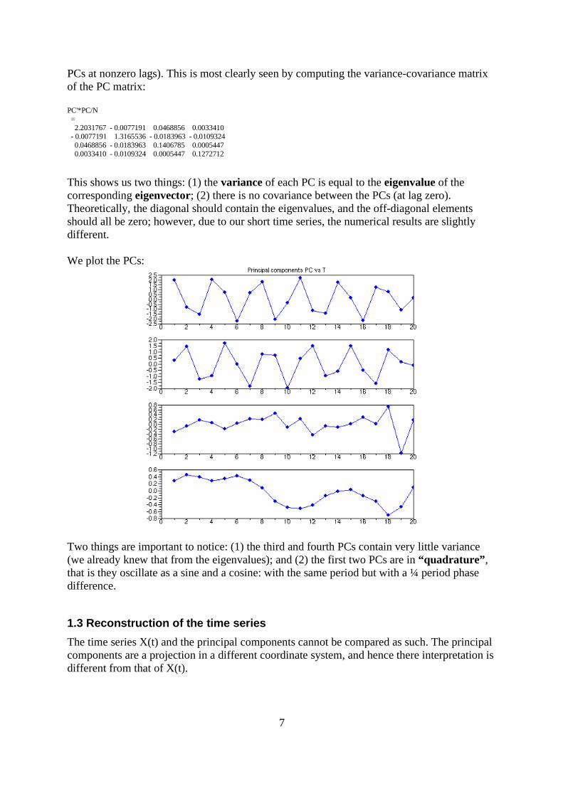
PCs at nonzero lags). This is most clearly seen by computing the variance-covariance matrix of the PC matrix:

PC'*PC/N = 2.2031767 - 0.0077191 0.0468856 0.0033410 - 0.0077191 1.3165536 - 0.0183963 - 0.0109324 0.0468856 - 0.0183963 0.1406785 0.0005447 0.0033410 - 0.0109324 0.0005447 0.1272712

This shows us two things: (1) the variance of each PC is equal to the eigenvalue of the corresponding eigenvector; (2) there is no covariance between the PCs (at lag zero). Theoretically, the diagonal should contain the eigenvalues, and the off-diagonal elements should all be zero; however, due to our short time series, the numerical results are slightly different.

We plot the PCs:

Two things are important to notice: (1) the third and fourth PCs contain very little variance (we already knew that from the eigenvalues); and (2) the first two PCs are in “quadrature”, that is they oscillate as a sine and a cosine: with the same period but with a ¼ period phase difference.

1.3 Reconstruction of the time series

The time series X(t) and the principal components cannot be compared as such. The principal components are a projection in a different coordinate system, and hence there interpretation is different from that of X(t).

7

However, by projecting the PCs back onto the eigenvectors, we obtain time series (referred to as the “reconstructed components”, RCs in SSA terminology) in the original coordinates (units), each one corresponding to one of the PCs. For this, we need to construct a matrix Z that is, like the matrix Y, an “embedded time series”, but that is different from Y in two ways: (i) we do not use X but one of the principal components; (ii) the time delay runs in the opposite direction. Note that we will construct a matrix Z for each one of the principal components.

For example, for the PC1, we obtain the following matrix Z:

Z = 1.9627574 0. 0. 0. - 0.8349101 1.9627574 0. 0. - 1.5315369 - 0.8349101 1.9627574 0. 2.0042159 - 1.5315369 - 0.8349101 1.9627574 0.7155270 2.0042159 - 1.5315369 - 0.8349101 - 2.2347452 0.7155270 2.0042159 - 1.5315369 0.6790097 - 2.2347452 0.7155270 2.0042159 1.8293911 0.6790097 - 2.2347452 0.7155270 - 2.0661013 1.8293911 0.6790097 - 2.2347452 - 0.3538360 - 2.0661013 1.8293911 0.6790097 2.2009377 - 0.3538360 - 2.0661013 1.8293911 - 1.1657792 2.2009377 - 0.3538360 - 2.0661013 - 1.4207885 - 1.1657792 2.2009377 - 0.3538360 1.7367143 - 1.4207885 - 1.1657792 2.2009377 0.1613329 1.7367143 - 1.4207885 - 1.1657792 - 2.1926827 0.1613329 1.7367143 - 1.4207885 1.2166946 - 2.1926827 0.1613329 1.7367143 0.7887929 1.2166946 - 2.1926827 0.1613329 - 1.115584 0.7887929 1.2166946 - 2.1926827 0.1576454 - 1.115584 0.7887929 1.2166946

Compare this matrix to PC1 (i.e., to the first column of the matrix PC). The first column of Z is simply PC1. The second column is PC1 at time t-1. The third column is PC1 at time t-2, and the last column is PC1 at time t-3. Note that, again, zeros have been put in where data was not available.

We obtain the RC1 (the first reconstructed component) by multiplying this matrix by the 1st

eigenvector and dividing by M. In Scilab code, RC1 = Z * RHO(:,1) /M. This operation is analogous to equation (11) for the first PC (K=1) and for the range M<t<N’ in Ghil et al (2002). (For values of t outside this range, see that paper, same paragraph; see also the copied text below right).

The Scilab script (see appendix) puts all the RCs together into a single matrix called RC, of which the columns are the reconstructed components: RC = 0.2964009 - 0.0190490 - 0.0499074 0.0259434 - 0.3064551 - 0.1400384 0.0055417 0.0852897 - 0.3349280 - 0.1243096 0.0167983 0.1494841 0.8165341 0.5192362 0.0462346 0.1831982

- 0.0614666 - 0.0597017 - 0.0146833 0.1797833 - 0.8186943 - 0.5117536 - 0.0084910 0.1733296 0.5448136 0.3401655 0.0136708 0.1715194 0.5272833 0.3510950 0.0562082 0.1479514

- 0.8799984 - 0.4809167 0.0704496 0.0664910 0.0708585 0.0206558 - 0.0720112 - 0.0516477 0.8310172 0.4728761 0.0365692 - 0.1588628 - 0.6577991 - 0.4524197 - 0.1702056 - 0.2165203

8

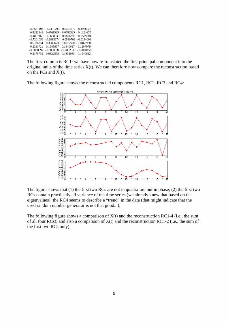
- 0.3631194 - 0.2301796 0.0453719 - 0.1976028 0.8323348 0.4761529 - 0.0786335 - 0.1324657 - 0.1807169 - 0.0608635 0.0806893 - 0.0579804 - 0.7201059 - 0.3815274 0.0530766 - 0.0234006 0.6326784 0.3980623 0.0075590 - 0.0460988 0.2331721 0.1989857 0.1340617 - 0.1287979 - 0.6838897 - 0.5090831 - 0.2882335 - 0.2068156 0.2375739 0.0822595 0.1352085 - 0.1940612

The first column is RC1: we have now re-translated the first principal component into the original units of the time series X(t). We can therefore now compare the reconstruction based on the PCs and X(t).

The following figure shows the reconstructed components RC1, RC2, RC3 and RC4:

The figure shows that (1) the first two RCs are not in quadrature but in phase; (2) the first two RCs contain practically all variance of the time series (we already knew that based on the eigenvalues); the RC4 seems to describe a “trend” in the data (that might indicate that the used random number generator is not that good...).

The following figure shows a comparison of X(t) and the reconstruction RC1-4 (i.e., the sum of all four RCs); and also a comparison of X(t) and the reconstruction RC1-2 (i.e., the sum of the first two RCs only).

9

The conclusion from these reconstructions is that we have reduced the time series to oscillatory components (corresponding to the first two eigenvalues) and two noise components (corresponding to the third and fourth eigenvalues). In fact, in the second figure, we have used the found RCs to “filter” the time series: by using less that the total number of RCs, we filter out a part of the time series that we suppose to be noise rather than signal. Here, we used the first two RCs, which we knew define an oscillatory signal due to the phase quadrature of the corresponding PCs, and their similar eigenvalues (although this remains to be verified by statistical tests!).

The filtered (=partially reconstructed) signal can now be analyzed further by using other spectral methods, e.g., to determine the dominant frequencies of the components of the time series. The SSA-MTM toolkit includes several such methods (BT, MEM, MTM).

1.4 How to interpret an SSA analysis.

Filtering of time series data. The eigenvectors of the matrix C (ie, the EOFs) can be used to reconstruct or “filter” the original time series. We say “filter” when the reconstruction is partial: i.e., we do not use all information, but only a selected portion, supposedly the essential portion of the time series. That is, we only use those eigenvectors that explain a large portion of the variance (measured by their eigenvalues). And in particular, we use the EOFS corresponding to the “paired” eigenvalues (see below).

An SSA reconstruction can be seen as follows. For a particular time t, we consider the observed values of X(t) that fall within the window of size M around t. Then the reconstructed value at time t is computed as a particular kind of weighted average of the values of X in this window. The EOFs define the “weights” for this averaging. A reconstruction hence corresponds to a kind of “moving average” of the time series. Note that the EOFS are such that when we take all of them into account, the moving average is identical to the original time series.

10

Eigenvalue pairs Why are pairs of eigenvalues indications of “ghost limit cycles” (regular but unstable oscillations underlying the noisy time series)? From Ghil et al 2002: “Vautard and Ghil [1989] argued that subject to certain statistical significance tests (...), such pairs correspond to the nonlinear counterpart of a sine-cosine pair in the standard Fourier analysis of linear problems.”

2. Multivariate Singular Spectral AnalysisThis section describes the differences between the univariate SSA and its multivariate extension, MSSA. For this reason we go through the same steps as in the previous case and clarify the differences.

2.1 How to compute EOFs and their eigenvalues

Now we consider the following 2-dimensional time series, stored in the matrix X:

X = 1.0135518 1.2441205 - 0.7113242 - 0.7790017 - 0.3906069 0.7752333 1.565203 1.4445798 0.0439317 - 0.4838554 - 1.1656093 - 0.8627650 1.0701692 0.6981061 1.0825379 - 0.7191011 - 1.2239744 - 2.0409115 - 0.0321446 0.3918897 1.1815997 1.1679199 - 1.4969448 - 0.3742759 - 0.7455299 - 0.1891236 1.0973884 1.8180156 - 0.2188716 - 0.4703280 - 1.0719573 - 1.0197255 0.9922009 0.9053288 0.4374216 - 0.0818220 - 1.6880219 - 1.3862948 0.2609807 - 0.0379891

The two time series look like this:

The first time series is the same as before; it was sampled from a sine function with period 3.3 and Gaussian noise was added. The second time series is sampled from the same sine function to the power of three and, again, Gaussian noise was added. An essential and necessary step for MSSA is to normalize both time series. That means to remove the mean value and to divide it by the standard deviation (for each series separately).

11

Next, we estimate the covariance matrix C including all auto- and cross-covariance functions of X. Therefore, we create a vector Y, which includes the time-delayed versions of the first and the second time series:

Y = 1.0135518 - 0.7113242 - 0.3906069 1.565203 1.2441205 - 0.7790017 0.7752333 1.4445798 - 0.7113242 - 0.3906069 1.565203 0.0439317 - 0.7790017 0.7752333 1.4445798 - 0.4838554 - 0.3906069 1.565203 0.0439317 - 1.1656093 0.7752333 1.4445798 - 0.4838554 - 0.8627650 1.565203 0.0439317 - 1.1656093 1.0701692 1.4445798 - 0.4838554 - 0.8627650 0.6981061 0.0439317 - 1.1656093 1.0701692 1.0825379 - 0.4838554 - 0.8627650 0.6981061 - 0.7191011 - 1.1656093 1.0701692 1.0825379 - 1.2239744 - 0.8627650 0.6981061 - 0.7191011 - 2.0409115 1.0701692 1.0825379 - 1.2239744 - 0.0321446 0.6981061 - 0.7191011 - 2.0409115 0.3918897 1.0825379 - 1.2239744 - 0.0321446 1.1815997 - 0.7191011 - 2.0409115 0.3918897 1.1679199 - 1.2239744 - 0.0321446 1.1815997 - 1.4969448 - 2.0409115 0.3918897 1.1679199 - 0.3742759 - 0.0321446 1.1815997 - 1.4969448 - 0.7455299 0.3918897 1.1679199 - 0.3742759 - 0.1891236 1.1815997 - 1.4969448 - 0.7455299 1.0973884 1.1679199 - 0.3742759 - 0.1891236 1.8180156 - 1.4969448 - 0.7455299 1.0973884 - 0.2188716 - 0.3742759 - 0.1891236 1.8180156 - 0.4703280 - 0.7455299 1.0973884 - 0.2188716 - 1.0719573 - 0.1891236 1.8180156 - 0.4703280 - 1.0197255 1.0973884 - 0.2188716 - 1.0719573 0.9922009 1.8180156 - 0.4703280 - 1.0197255 0.9053288 - 0.2188716 - 1.0719573 0.9922009 0.4374216 - 0.4703280 - 1.0197255 0.9053288 - 0.0818220 - 1.0719573 0.9922009 0.4374216 - 1.6880219 - 1.0197255 0.9053288 - 0.0818220 - 1.3862948 0.9922009 0.4374216 - 1.6880219 0.2609807 0.9053288 - 0.0818220 - 1.3862948 - 0.0379891 0.4374216 - 1.6880219 0.2609807 0. - 0.0818220 - 1.3862948 - 0.0379891 0. - 1.6880219 0.2609807 0. 0. - 1.3862948 - 0.0379891 0. 0. 0.2609807 0. 0. 0. - 0.0379891 0. 0. 0.

The first four columns are identical to Y in the univariate case, where the second four columns represent the time-delayed embedding of the second time series.

The covariance matrix C can be derived from this matrix as Y'*Y/N:

C = 1. - 0.2867228 - 0.6546009 0.6872825 0.783843 - 0.5205869 - 0.4463800 0.6902719 - 0.2867228 0.9486356 - 0.2506746 - 0.6348058 0.0045700 0.7207940 - 0.4811090 - 0.4856669 - 0.6546009 - 0.2506746 0.9233365 - 0.2645671 - 0.7143745 0.0488186 0.6930878 - 0.4535369 0.6872825 - 0.6348058 - 0.2645671 0.9157079 0.5050230 - 0.6900764 0.0336045 0.7082284 0.783843 0.0045700 - 0.7143745 0.5050230 1. - 0.1315155 - 0.4998541 0.5150921 - 0.5205869 0.7207940 0.0488186 - 0.6900764 - 0.1315155 0.9226082 - 0.0830569 - 0.5480783 - 0.4463800 - 0.4811090 0.6930878 0.0336045 - 0.4998541 - 0.0830569 0.8922660 - 0.0528615 0.6902719 - 0.4856669 - 0.4535369 0.7082284 0.5150921 - 0.5480783 - 0.0528615 0.8622167

The matrix C has dimension L·M, where L is the number of variables in the time series. In our case, L=2.

Question: does the way we have computed C here correspond to the first or the second method as described above for SSA?

We compute the eigenvalues (λ) and eigenvectors (ρ) of the matrix C. [In Scilab, use the function spec(C)]

LAMBDA = 3.9351181 2.4195975 0.4599736 0.2790406 0.1316975 0.1012908 0.0736324 0.0644204

12

RHO = 0.4730634 - 0.1054322 - 0.0901056 0.2175589 0.4720963 - 0.6274409 0.1806476 - 0.2458731 - 0.2249794 - 0.5297505 - 0.0108227 - 0.1051553 - 0.4298665 - 0.5431790 - 0.4194785 - 0.0422269 - 0.3177635 0.4190955 0.0273376 0.4765846 0.0515316 - 0.3711261 - 0.1102094 0.5856355 0.4162558 0.2331546 0.1292536 0.1669875 - 0.7518224 - 0.1311260 0.3801923 - 0.0283132 0.3893586 - 0.2904463 0.4888841 0.4841341 0.0433365 0.3057310 - 0.4275540 0.1117829 - 0.3232252 - 0.3566756 0.6146423 - 0.0415173 0.1155326 - 0.0816922 0.5921959 0.1344684 - 0.1638748 0.5034736 0.5524014 - 0.1395248 0.0386233 - 0.1794367 - 0.2809422 - 0.5314388 0.4103939 0.1148223 0.2288447 - 0.6565182 0.0879197 - 0.1549298 - 0.1492819 0.5300835

The covariance matrix has size 2·M × 2·M, therefore we get 8 eigenvalues and eigenvectors. The columns of RHO contain the eigenvectors, where each has length 8. The first 4 components of each eigenvector belong to the first time series and the second 4 components to the second time series. We plot the first pair of eigenvectors:

The first four values of the eigenvectors are similar to the eigenvectors obtained with SSA (compare the figure in section 1.1). However, due to estimation problems in the covariance matrix (because of the shortness of the time series), the eigenvectors are not symmetric or antisymmetric as before.

2.2 Principal components

Once we have determined the eigenvectors we compute the principal components as:

PC = Y*RHO

This gives:

PC = 2.6171605 0.9438761 0.9962493 - 0.0513752 - 0.2917500 - 0.2287511 - 0.3070882 - 0.1041581 - 1.716888 1.5696349 0.8996988 0.3463854 - 0.0512167 - 0.4139074 0.3380974 0.0997600 - 1.4759344 - 2.1244232 0.6709754 0.5259982 0.1273124 - 0.1290738 - 0.3863778 0.1693864 2.6931466 - 1.0284971 0.0569486 0.3406141 - 0.1098447 - 0.1858399 0.0336523 - 0.1746411 0.0745299 2.0309225 - 0.3679344 0.9991928 - 0.3938383 - 0.0248507 0.3976838 - 0.2877883 - 2.9269561 - 0.8705194 - 0.8921540 0.9389603 - 0.1982590 0.0332216 0.0448624 0.2077649 1.6377916 - 2.135586 - 1.284177 - 0.0743977 - 0.0962281 - 0.2233394 - 0.3475563 0.2489629 2.0843124 2.0645034 - 1.0546837 - 0.5386314 - 0.0019376 - 0.4617901 - 0.0238460 - 0.2107538 - 2.8366751 1.2902979 - 0.2479362 - 0.8713252 0.5913432 - 0.2643676 - 0.0745443 0.0421521 - 0.3568950 - 2.1642956 0.5122341 - 0.6515377 0.0810931 0.1525250 0.0375361 - 0.5980391 2.9422599 0.5196485 0.6836954 - 0.3437828 0.4977630 0.3444301 0.4015147 0.4494413 - 1.5557823 1.9991321 0.7420831 0.1209452 - 0.1743242 0.6133022 - 0.5543623 - 0.2343394 - 1.9789113 - 1.7917956 0.4425631 0.0071434 0.0649748 0.1295294 0.4634063 - 0.0281263 2.7205448 - 0.9874034 0.2460260 0.3641712 - 0.1243806 0.3350277 - 0.1190721 0.2453557

13

- 0.0310430 2.0554902 - 0.2603362 0.3530523 - 0.0306845 0.0837419 - 0.1778383 - 0.0464315 - 2.8171564 - 0.8499547 - 0.4248928 - 0.0206860 0.2944135 0.0363924 - 0.0977785 - 0.1579876 1.6065225 - 1.9190181 - 0.4887260 0.0690209 - 0.0299186 0.2702111 0.2406166 - 0.4515899 0.9262209 1.4565839 - 0.9270728 0.4202916 0.7804026 0.6406357 - 0.0169565 - 0.0588009 - 1.3847434 0.4559112 - 0.5518115 - 1.064263 - 0.9735619 0.4966449 0.1558060 0.2439464 0.1086690 - 0.0164820 - 0.0420881 0.0383868 0.1215617 - 0.1753644 0.0633879 - 0.0684147

By writing down element-by-element the results of this matrix product (try this!) one discovers that each element of the PC matrix is the sum of a linear combination of M values of the first time series (weighted by that part of the EOF that corresponds to the first time series) and a linear combination of the M values of the second time series (again weighted by the corresponding part of the EOF). This means that each PC contains characteristics of both time series. Unlike the EOFs or the matrices Y and C, we can no longer identify a part that corresponds to each separate time series.

The first 4 PCs are shown here:

2.3 Reconstruction of the time series

Analogously to the univariate SSA, each time series can be reconstructed by projecting the PCs back onto the eigenvectors. As before, we embed each PC time-delayed with delays 0...-M+1, what yields to a matrix Z of size N×M with the same structure. In order to reconstruct the first time series we use the first M rows of RHO, and for the second time series the second M rows.

14

In Scilab this means to calculate RCx1(:,m)=Z*RHO(1:M,m)/M and RCx2(:,m)=Z*RHO(M+1:2*M,m)/M, respectively. Note that we use the same matrix Z for both time series. The information specific to each of the two variables in X(t) is hence contained in the eigenvectors. This gives the following RCs:

The first both RC1 and RC2 describe the oscillations, where the RC3 and RC4 describe a trend (which may be introduced due to the random number generator and the very short time series). When we summarize all eight RCs we reconstruct the whole time series:

15

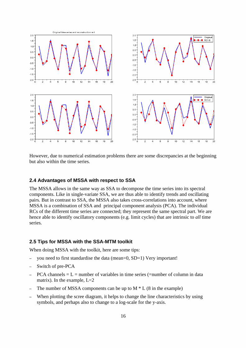
However, due to numerical estimation problems there are some discrepancies at the beginning but also within the time series.

2.4 Advantages of MSSA with respect to SSA

The MSSA allows in the same way as SSA to decompose the time series into its spectral components. Like in single-variate SSA, we are thus able to identify trends and oscillating pairs. But in contrast to SSA, the MSSA also takes cross-correlations into account, where MSSA is a combination of SSA and principal component analysis (PCA). The individual RCs of the different time series are connected; they represent the same spectral part. We are hence able to identify oscillatory components (e.g. limit cycles) that are intrinsic to all time series.

2.5 Tips for MSSA with the SSA-MTM toolkit

When doing MSSA with the toolkit, here are some tips:

– you need to first standardise the data (mean=0, SD=1) Very important!

– Switch of pre-PCA

– PCA channels = L = number of variables in time series (=number of column in data matrix). In the example, L=2

– The number of MSSA components can be up to M * L (8 in the example)

– When plotting the scree diagram, it helps to change the line characteristics by using symbols, and perhaps also to change to a log-scale for the y-axis.

16

3. Glossary (under construction)EOF: Empirical orthogonal function = eigenvectorsMSSA: Multichannel SSA; as SSA but for multivariate time series Nyquist interval: the minimum required interval (i.e., number of data points of time series)

that is required to reconstruct a sinusoidal signal from the data points. Scree diagram: a graph plotting the eigenvalues of the covariance matrix C versus their rank

(i.e., ranked by their value) and usually including error bars. Is used to visually distinguish between important and other EOFs, by assessing the change in the slope of the scree diagram. Pairs of eigenvalues might also be distinguished, although the significance of the pairing needs to be established statistically. Note: a Scree diagram is not a power spectrum: although the eigenvalues correspond to “power”, the eigenvalues are not plotted against frequency but simply against rank.

SSA components : the number of EOFs retained by the Toolkit for further analysisSSA eigenspectrum : Scree diagramPower spectrum: the distribution of frequencies present in the time series; “power” refers to

the weight that each frequency has in the time series. Thus, peaks in the power spectrum correspond to dominant frequencies in the time series. NB a Scree diagram is not a power spectrum.

4. ReferencesGhil M., R. M. Allen, M. D. Dettinger, K. Ide, D. Kondrashov, M. E. Mann, A. Robertson, A.

Saunders, Y. Tian, F. Varadi, and P. Yiou, 2002: "Advanced spectral methods for climatic time series," Rev. Geophys.,40(1), pp. 3.1-3.41, 10.1029/2000RG000092.

5. APPENDIX: The Scilab scripts

A.1 Scilab instructions1. To start Scilab and Scipad: open a terminal; enter “scilab”; in the appearing scilab

window enter “scipad”. Scipad is the editor that you can use to read, write and execute scilab scripts.

2. In Scipad, click “Open file”; select the SSA script (download the script from the atelier website, see link to TD data; the script has extension .sci)

3. Hit F5 to run the script. The script runs stepwise; you need to hit a key in the scilab window to continue after each step

4. Try to understand what is going on.

A.2 The Scilab script for doing the SSA computations used in this guide

17

//=========================================================

// SSA beginner's guide//// This guide demonstrates step by step the singular spectral// analysis.//=========================================================

clear; // clear workspace// mode(-1); // no output in the consolemode(0); // standard ouput in the console

//-- Set general Parameters ------------------------------- M = 4; // embedding dimension N = 20; // length of generated time series waitforkeypress = %T; // wait for keypress (%T/%F)//---------------------------------------------------------

clc;function waithere if waitforkeypress halt('Press <Enter> to continue...'); disp(''); end;endfunctionlines(0);

//---------------------------------------------------------// Create time series X//// First of all, we generate a time series, a sine function// of length N with observational noise//---------------------------------------------------------t = (1:N)';X = sin(2*%pi*t/3.3); // sine function with period length 3.3rand('seed',0.123456789);rand('normal');noise = 0.2*rand(X); // Gaussian noiseX = X+noise;X = X-mean(X); // remove mean valuestdX = sqrt(X'*X /N); X = X/stdX; // normalize to std=1X

clf;plot(X, 'r.-');xtitle('Time series X(t) vs T');waithere;

//---------------------------------------------------------// Calculate covariance matrix C//// Next, we calculate the covariance matrix. There are// several numerical approaches to estimate C. Here,// we calculate the covariance function with CORR and// build C with the function TOEPLITZ.//---------------------------------------------------------covX = corr(X,M)

Ctoep=toeplitz(covX);Ctoepwaithere;

//---------------------------------------------------------// Calculate covariance matrix (alternative estimation)//// An alternative approach is to determine C directly from// the scalar product of Y, the time-delayed embedding of X.// However, this estimation of C is biased and does not give a// Toeplitz structure. Therefore, the eigenvectors wouldn't be// symmetric or antisymmetric. //---------------------------------------------------------Y=zeros(N,M);for m=1:M // create time-delayed embedding of X Y((1:N-m+1),m) = X((1:N-m+1)+m-1);

18

end;Ywaithere;Cemb=Y'*Y / N;Cembwaithere;

//---------------------------------------------------------// We proceed with C=Ctoep!//---------------------------------------------------------

C=Ctoep;

//---------------------------------------------------------// Calculate eigenvalues LAMBDA and eigenvectors RHO//// In order to determine the eigenvalues and eigenvectors of C// we use the function SPEC. This function returns two matrices,// the matrix RHO with eigenvectors arranged in columns, and the// matrix LAMBDA with eigenvalues on the diagonal.//---------------------------------------------------------[RHO,LAMBDA] = spec(C);LAMBDA = diag(LAMBDA); // extract the diagonal[LAMBDA,ind]=gsort(LAMBDA); // sort eigenvaluesRHO = RHO(:,ind); // and eigenvectorsLAMBDA

clf;xtitle('Eigenvectors RHO')plot(RHO, '.-','LineWidth',2);legend('1', '2', '3', '4');

waithere;

//---------------------------------------------------------// Calculate principal components PC//// The principal components are given as the scalar product// between Y, the time-delayed embedding of X, and the// eigenvectors RHO.(//---------------------------------------------------------PC = Y*RHO;

clf;xtitle('Principal components PC vs T')for m=1:M subplot(M,1,m); plot(PC(:,m),'.-');end;PCwaithere;

//---------------------------------------------------------// Calculate reconstructed components RC//// In order to determine the reconstructed components RC,// we have to calculate the scalar product between PCtde// (Z=the time-delayed embedding of the principal components PC)// and the eigenvectors.//---------------------------------------------------------RC=zeros(N,M);for m=1:M Z=zeros(N,M); // time-delayed embedding of PC(:,m): // Note the difference to Y! for m2=1:M Z((1:N-m2+1)+m2-1,m2) = PC((1:N-m2+1),m); end; // determine RC as a scalar product RC(:,m) = Z * RHO(:,m) /M;end;

RC

19

clf;xtitle('Reconstructed components RC vs T')for m=1:M subplot(M,1,m); plot(RC(:,m),'r.-');end;waithere;

//---------------------------------------------------------// Compare reconstruction and original time series//// Beside some numerical estimation problems at the beginning,// the original time series X can be completely reconstructed// by the sum of all reconstructed components RC.//---------------------------------------------------------//figure(5,'Figure_name','Full reconstruction and original time series'); clf;xtitle('Original time series and reconstruction vs T')subplot(2,1,1)plot(t,X,'b','LineWidth',2);plot(t,sum(RC,2),'r.-');legend('Original','RC1-4');

subplot(2,1,2)plot(t,X,'b','LineWidth',2);plot(t,RC(:,1)+RC(:,2),'r.-');legend('Original','RC1-2');

disp('Script finished');

A.3 The Scilab script for doing the MSSA computations used in this guide

//=========================================================// MSSA beginner's guide//// This guide demonstrates step by step the multivariate// singular spectral analysis. The steps are almost similar// to a singular spectral analysis//=========================================================

clear; // clear workspace// mode(-1); // no output in the consolemode(0); // standard ouput in the console

//-- Set general Parameters ------------------------------- M = 4; // embedding dimension N = 20; // length of generated time series waitforkeypress = %T; // wait for keypress (%T/%F)//---------------------------------------------------------

clc;function waithere if waitforkeypress halt('Press <Enter> to continue...'); disp(''); end;endfunctionlines(0);

//---------------------------------------------------------// Create time series X//// First of all, we generate two time series, a sine function// of length N and the same function to the power of 3, both// with observational noise//---------------------------------------------------------t = (1:N)';X1 = sin(2*%pi*t/3.3); // sine function with period length 3.3X2 = X1.^3;rand('seed',0.123456789);rand('normal');noise = 0.2*rand(N,2); // Gaussian noise

20

X1 = X1+noise(:,1);X2 = X2+noise(:,2);X1 = X1-mean(X1); // remove mean valueX2 = X2-mean(X2);stdX1 = sqrt(X1'*X1 /N); stdX2 = sqrt(X2'*X2 /N); X1 = X1/stdX1; // normalize to std=1X2 = X2/stdX2;X = [X1 X2]

clf;subplot(1,2,1);plot(X1, 'r.-');xtitle('Time series X1(t) vs t');subplot(1,2,2);plot(X2, 'r.-');xtitle('Time series X2(t) vs t');waithere;

//---------------------------------------------------------// Calculate covariance matrix//// Here we use only the "alternative" approach for simplicity.// This means to determine C directly from// the scalar product of Y, the time-delayed embedding of X.// However, this estimation of C is biased and does not give a// Toeplitz structure. Therefore, the eigenvectors wouldn't be// symmetric or antisymmetric. //---------------------------------------------------------Y1=zeros(N,M);Y2=zeros(N,M);for m=1:M // create time-delayed embedding of X Y1((1:N-m+1),m) = X1((1:N-m+1)+m-1); Y2((1:N-m+1),m) = X2((1:N-m+1)+m-1);end;Y = [Y1 Y2]waithere;Cemb=Y'*Y / N;Cembwaithere;

C=Cemb;

//---------------------------------------------------------// Calculate eigenvalues LAMBDA and eigenvectors RHO//// In order to determine the eigenvalues and eigenvectors of C// we use the function SPEC. This function returns two matrices,// the matrix RHO with eigenvectors arranged in columns, and the// matrix LAMBDA with eigenvalues on the diagonal.//---------------------------------------------------------[RHO,LAMBDA] = spec(C);LAMBDA = diag(LAMBDA); // extract the diagonal[LAMBDA,ind]=gsort(LAMBDA); // sort eigenvaluesRHO = RHO(:,ind); // and eigenvectorsLAMBDA

clf;xtitle('Eigenvectors RHO')plot(RHO(:,1:2), '-','LineWidth',2);legend('1', '2');

waithere;//---------------------------------------------------------// Calculate principal components PC//// The principal components are given as the scalar product// between Y, the time-delayed embedding of X1 and X2, and the// eigenvectors RHO.//---------------------------------------------------------PC = Y*RHO;

clf;xtitle('Principal components PC vs t')

21

for m=1:M subplot(M,1,m); plot(PC(:,m),'.-');end;PCwaithere;

//---------------------------------------------------------// Calculate reconstructed components RC//// In order to determine the reconstructed components RC,// we have to calculate the scalar product between PCtde// (Z=the time-delayed embedding of the principal components PC)// and the eigenvectors.//---------------------------------------------------------RC1=zeros(N,M);RC2=zeros(N,M);for m=1:M Z=zeros(N,M); // time-delayed embedding of PC(:,m): // Note the difference to Y! for m2=1:M Z((1:N-m2+1)+m2-1,m2) = PC((1:N-m2+1),m); end; // determine RC as a scalar product RC1(:,m) = Z * RHO(1:M,m) /M; RC2(:,m) = Z * RHO(M+1:2*M,m) /M;end;

RC = [RC1 RC2]

clf;xtitle('Reconstructed components RC vs T')for m=1:M subplot(M,2,2*m-1); plot(RC1(:,m),'r.-'); subplot(M,2,2*m); plot(RC2(:,m),'r.-');end;waithere;

//---------------------------------------------------------// Compare reconstruction and original time series//// Beside some numerical estimation problems at the beginning,// the original time series X can be completely reconstructed// by the sum of all reconstructed components RC.//---------------------------------------------------------//figure(5,'Figure_name','Full reconstruction and original time series'); clf;xtitle('Original time series and reconstruction vs t')subplot(2,2,1)plot(t,X1,'b','LineWidth',2);plot(t,sum(RC1,2),'r.-');subplot(2,2,2)plot(t,X2,'b','LineWidth',2);plot(t,sum(RC2,2),'r.-');legend('Original','RC1-8');

subplot(2,2,3)plot(t,X1,'b','LineWidth',2);plot(t,RC1(:,1)+RC1(:,2),'r.-');subplot(2,2,4)plot(t,X2,'b','LineWidth',2);plot(t,RC2(:,1)+RC2(:,2),'r.-');legend('Original','RC1-2');

disp('Script finished');

22