A Bayesian hybrid method for context-sensitive spelling correction

A n d r e w It. Gold ing Mitsubishi Electric Research Labs

201 Broadway, 8th Floor Cambridge, MA 02139

golding©merl, tom

A b s t r a c t

Two classes of methods have been shown to be useful for resolving lexical ambiguity. The first relies on tile presence of particular words within some distance of tile ambiguous target word; the second uses the pattern of words and part-of-speech tags around the target word. These methods have complementary coverage: the former captures the lexical "atmosphere" (discourse topic, tense, etc.), while tile latter captures local syntax. Yarowsky has exploited this complementarity by combining the two methods using decision lists. The idea is to pool the evidence provided by the component methods, and to then solve a target problem by applying the single strongest piece of evidence, whatever type it happens to be. This paper takes Yarowsky's work as a starting point, applying decision lists to the problem of context-sensitive spelling correction. Decision lists are found, by and large, to outperform either component method. However, it is found that further improvements can be obtained by taking into account not just the single strongest piece of evidence, but all the available evidence. A new hybrid method, based on Bayesian classifiers, is presented for doing this, and its performance improvements are demonstrated.

1 In troduc t ion

Two classes of methods have been shown useful for resolving lexical ambiguity. The first tests for the presence of particular c o n t e x t words within a certain distance of the ambiguous target word. The second tests for co l loca t ions - - patterns of words and part-of-speech tags around the target word. The context-word and collocation methods have complementary coverage: the former captures the lexical "atmosphere" (discourse topic, tense, etc.), while the latter captures local syntax. Yarowsky [1994] has exploited this complementarity by combining the two methods using decision lists. The idea is to pool the evidence provided by the component methods, and to then solve a target problem by applying the single strongest piece of evidence, whatever type it happens to be. Yarowsky applied his method to the task of restoring missing accents in Spanish and French, and found that it outperformed both the method based on context words, and one based on local syntax. This paper takes Yarowsky's method as a starting point, and hypothesizes that further improvements can be obtained by taking into account not only the single strongest piece of evidence, but all the available evidence. A method is presented for doing this, based on Bayesian classifiers.

The work reported here was applied not to accent restoration, but to a related lexical disam- biguation task: context-sensitive spelling correction. The task is to fix spelling errors that happen to result in valid words in the lexicon; for example:

I'd like the chocolate cake for ,desert.

where d e s s e r t was misspelled as deser t . This goes beyond the capabilities of conventional spell checkers, which can only detect errors that result in non-words.

39

We start by applying a very simple method to the task, to serve as a baseline for comparison with the other methods. We then al)ply each of the two component methods mentioned above - - context words and collocations. We try two ways of combining these components: decision lists, and Bayesian classifiers. We evaluate the above methods by comparing them with an alternative approach to spelling correction based on part-of-speech trigrams.

The sections below discuss the task of context-sensitive spelling correction, the five methods we tried for the task (baseline, two component methods, and two hybrid methods), and the evaluation. The final section draws some conclusions.

2 Context -sens i t ive spell ing correction

Context-sensitive spelling correction is the problem of correcting spelling errors tha t result in valid words in the lexicon. Such errors can arise for a. variety of reasons, including typos (e.g., out for our), homonym confusions (there for their), and usage errors (between for among). These errors are not detected by collventional spell checkers, as they only notice errors resulting in non-words.

We treat context-sensitive spelling correction as a task of word disambiguation. The ambiguity among words is modelled by eonfusio~ sets. A confilsion set C = { w l , . . . , Wn} means that each word wi in the set is ambiguous with each other word in the set. Thus if C = {desert, dessert}, then when the spelling-correction program sees an occurrence of either desert or dessert in the target document, it takes it to be a.mbiguous between desert and dessert, and tries to infer fi'om the context which of the two it should be.

This t rea tment requires a collection of confusion sets to start with. There are several ways t o obtain such a collection. One is based on finding words in the dictionary tha t are one typo away from each other [Mays et al., 1991]. 1 Another finds words that have the same or similar pronunciations. Since this was not the focus of the work reported here, we simply took (most of) our confusion sets fl'om the list of "Words Commonly Confused" in the back of the Random House unabridged dictionary [Flexner, 1983].

A final point concerns the two types of errors a spelling-correction program can make: false negatives (complaining about a correct word), and false positives (failing to notice an error). We will make the simplifying assumption that both kinds of errors are equally bad. In practice, however, false negatives are much worse, as users get irr i tated by programs that badger them with bogus complaints. However, given the probabilistic nature of the methods that will be presented below, it would not be hard to modify them to take this into account. We would merely set a confidence threshold, and report a suggested correction only if the probability of the suggested word exceeds the probability of the user's original spelling by at least the threshold amount. The reason this was not done in the work reported here is that setting this confidence threshold involves a certain

subjective factor (which depends on the user's "irritability threshold"). Our simpli~,ing assumption allows us to measure performance objectively, by the single parameter of prediction accuracy.

1Constructing confllsion sets in this way requires assigning each word in the lexicon its own confusion set. For instance, cat might have the confusion set {hat, car,...}, hat might have {cat, had . . . . }, and so on. We cannot u s e

t h e symmetric conflmion sets that we have adopted -- where every word in the set is confusable with every o t h e r o n e

- - b e c a u s e t h e "confusable" relation is no longer transitive.

40

3 Five m e t h o d s for spel l ing correct ion

This section presents a progression of five methods for context-sensitive spelling correction:

B a s e l i n e An indicator of "minimal competency" for comparison with the other methods C o n t e x t w o r d s Tests for particular words within ::t=k words of the ambiguous target word C o l l o c a t i o n s Tests for syntactic pat terns around the ambiguous target word D e c i s i o n l i s t s Combines context words and collocations via decision lists B a y e s i a n c lass i f ie rs Combines context words and collocations via Bayesian classifiers.

Each method will be described in terms of its operation on a single confusion set C = ( W l , . . . , w~}; that is, we will say how the method disambiguates occurrences of words wl through wn from the context. The methods handle multiple confusion sets by applying the same technique to each confusion set independently.

Each method involves a training phase and a test phase. The performance figures given below are based on training each method on the 1-million-word Brown corpus [Ku~:era and Francis, 1967] and testing it on a 3/4-million-word corpus of Wall Street Journal text [Marcus et al., 1993].

3 .1 B a s e l i n e m e t h o d

The baseline method disambiguates words wl through wn by simply ignoring the context, and always guessing that the word should be whichever wi occurred most often in the training corpus. For instance, if C -- (desert, dessert}, and desert occurred more often than dessert in the training corpus, then the method will predict that every occurrence of desert or dessert in the test corpus should be changed to (dr left as) desert.

Table 1 shows the performance of the baseline method for 18 confusion sets. This collection of confusion sets will be used for evaluating the methods throughout the paper. Each line of the table gives the results for one confusion set: the words in the confusion set; the number of instances of any word in the confusion set in the training corpus and in the test corpus; the word in the confusion set that occurred most often in the training corpus; and the prediction accuracy of the baseline method for the test corpus. Prediction accuracy is the number of times the correct word was predicted, divided by the total number of test cases. For example, the members of the confusion set {I, me} occurred 840 times in the test corpus, the breakdown being 744 I and 96 me. The baseline method predicted I every time, a.nd thus was right 744 times, for a score of 744/840 = 0.886.

Essentially the baseline method measures how accurately one can predict words using just their prior probabilities. This provides a lower bound on the performance we would expect from the other methods, which use more than just the priors.

3 .2 C o m p o n e n t m e t h o d 1: C o n t e x t w o r d s

One clue about the identity of an ambiguous target word comes from the words around it. For instance, if the target word is ambiguous between desert and dessert, and we see words like arid, sand, and sun nearby, this suggests that the target word should be desert. On the other hand, words such as chocolate and delicious ill the context imply dessert. This observation is the basis for the method of context words. The idea is that each word wi in the confusion set will have a characteristic distribution of words that occur in its context; thus to classify an ambiguous target word, we look at the set of words around it and see which wi's distribution they most closely follow.

41

Confusion set No. of

training cases

No. of

test cases

whether, weather 331 245 I, me 6125 840 its, it 's 1951 3575 past, passed 385 397 than, then 2949 1659 being, begin 727 449 effect, affect 228 162 your, you're 1047 212 number, amount 588 429 council, counsel 82 83 rise, raise 139 301 between, among 1003 730 led, lead 226 219 except, accept 232 95 peace, piece 310 61 there, their, they're 5026 2187 principle, principal 184 69 sight, site, cite 149 44

Most frequent word

Baseline

whether 0.922 I 0.886 its 0.863 past 0.861 than 0.807 being 0.780 effect 0.741 your 0.726 number 0.627 council 0.614 rise 0.575 between 0.538 led 0.530 except 0.442 peace 0.393 there 0.306 principle 0.290 sight 0.114

Table 1: Performance of the baseline method for 18 confusion sets. The "Most frequent word" column gives the word in the confusion set that occurred most frequently in the training corpus. (In subsequent tables, confusion sets will be referred to by their most frequent word.) The "Baseline" column gives the prediction a,ccuracy of the baseline system on the test corpus.

Following previous work [Gale et al., 1994], we formulate tile method in a Bayesian framework. The task is to pick the word wi that is most probable, given the context words cj observed within a =t:k-word window of the target word. The probabil i ty for each wi is calculated using Bayes' rule:

p(wi lc -k , . . . , C-1, e l , . . . , Ck) = P ( C - k ' ' ' " C- l ' C l ' ' " ' CklWi) p(wi) p ( C - k , . . . , C - l , C l , . . . ,Ck)

As it stands, the likelihood term, p ( c - k . . . . , C-l, C l , . . . , CklWi) , is difficult to es t imate from training da ta - - we would have to count situations in which the entire context was previously observed around word wi, which raises a severe sparse-data problem. Instead, therefore, we assume that the presence of one word in the context is independent of the presence of any other word. This lets us decompose the likelihood into a product:

p(c_k,...,c_1,cl,.. ,cklw ) = lII p(cjlw ) j 6 - k . . . . . - 1 , 1 . . . . . k

Gale et al. [1994] provide evidence that this is in fact a reasonable approximation. We still have the problem, however, of est imating the individual p(c j lw i ) probabilit ies from our

training corpus. The straightforward way would be to use a. maximum likelihood est imate - - we

4 2

would count Mi, the total number of occurrences of wi in the training corpus, and mi, the number of such occurrences for which cj occurred within ±k words, and we would then take the ratio mi/~4i.2 Unfortunately, we may not have enough training da ta to get an accurate est imate this way. Gale et al. [1994] address this problem by interpolating between two maximum-likefihood estimates: one of p(cjlwi) , and one of p(cj). The former measures the desired quantity, but is subject to inaccuracy due to sparse data; the lat ter provides a robust estimate, but of a potentially irrelevant quantity. Gale et al. interpolate between the two so as to minimize the overall inaccuracy.

We have pursued an alternative approach to the problem of est imating the likelihood terms. We start with the observation that there is no need to use every word in the ±k-word window to discriminate among the words in the confusion set. If we do not have enough training da ta for a given word c to accurately est imate p(clwi ) for all w/, then we simply disregard e, and base our discrimination on other, more reliable evidence. We implement this by introducing a "minimum occurrences" threshold, Train. It is currently set to 10. We then ignore a context word c if:

l < i < n l < i < n

where mi and Mi are defined as above. In other words, e is ignored if it practically never occurs within the context of any wi, or if it practically always occurs within the context of every wi. In the former case, we have insufficient da ta to measure its presence; in the latter, its absence.

Besides the reason of insufficient data, a second reason to ignore a context word is if it does not help discriminate among the words in the confusion set. For instance, if we are trying to decide between I and me, then the presence of the in the context probably does not help. By ignoring such words, we eliminate a source of noise in our discrimination procedure, as well as reducing storage requirements and run time. To determine whether a context word e is a useful discriminator, we run a chi-squa.re test [Fleiss, 1981] to check for an association between the presence of c and the choice of word in the confusion set. If the observed association is not judged to be significant, a then c is discarded. The significance level is currently set to 0.05.

Figure 1 pulls together the points of the preceding discussion into an outline of the method of context words. In the training phase, it identifies a list of context words that are useful for discriminating among the words in the confusion set. At run time, it est imates the probabili ty of each word in the confusion set. It s tarts with the prior probabilities, and multiplies them by the likelihood of each context word fl'om its list that appears in the ±k-word window of the target word. Finally, it selects the word in the confusion set with the greatest probability.

The main parameter to tune for the method of context words is k, the half-width of the context window. Previous work [Yarowsky, 1994] shows that smaller values of k (3 or 4) work well for resolving local syntactic ambiguities, while larger values (20 to 50) are suitable for resolving semantic ambiguities. We tried the values 3, 6, 12, and 24 on some practice confusion sets (not shown here), and found that k = 3 generally did best, indicating that most of the action, for our task and confusion sets, comes fl'om local syntax. In the rest of this paper, this value of k will be used.

=We are i n t e rp re t i ng the condi t ion "cj occurs wi th in a =l=k-word window of wi" as a b ina ry fea ture - - e i ther i t happens , or i t does not . Th i s allows us to handle con tex t words in the same Bayesian f r amework as will be used la ter for o the r b inary features (see Section 3.3). A more convent ional i n t e rp r e t a t i on is to take in to account the number of occurrences of each cj with in the ::l=k-word window, and to e s t ima te p(cjlwi ) accordingly. However, e i ther i n t e r p r e t a t i o n is valid, as long as i t is applied cons is tent ly - - t h a t is, b o t h when e s t ima t ing the l ikel ihoods from t r a in ing da ta , and when classifying test. cases.

3An associa t ion is significant if the probabi l i ty t h a t i t occurred by chance is low. Th i s is no t a s t a t e m e n t abou t the strength of the associat ion. Even a weak associat ion may be judged signif icant if there are enough d a t a to suppor t it. Measures of the s t r eng th of associat ion will be discussed in Section 3.4.

4 3

Training phase

(1) Propose all words as candidate context words. (2) Count occurrences of each candidate context word in the training corpus. (3) Prune context words that have insufficient da ta or are uninformative discriminators. (4) Store the remaining context words (and their associated statistics) for use at run time.

Run time

(1) Initialize the probability for each word in the confusion set to its prior probability. (2) Go through the list of context words that was saved during training. For each context word

tha t appears in the context of the ambiguous target word, update the probabilities. (3) Choose the word in the confusion set with the highest probability.

Figure 1: Outline of the method of context words.

Table 2 shows the effect of varying k for our usual collection of confusion sets. It can be seen that performance generally degrades as k increases. The reason is that the method starts picking up spurious correlations in the training corpus. Table 4 gives some examples of the context words learned for the confusion set {peace, piece}, with k = 24. The context words coTTs, united, nations, etc., all imply peace, and appear to be plausible (although united and nations are a counterexample to our earlier assumption of independence). On the other hand, consider the context word how, which allegedly also implies peace. If we look back at the training corpus for the supporting data for this word, we find excerpts such as:

But oh, how I do sometimes need just a moment of rest, and peace . . . No mat te r how earnest is our quest for guaranteed peace . . .

How best to destroy your peace ?

There does not seem to be a necessary connection here between how and peace; the correlation is probably spurious. Although we are using a chi-square test expressly to filter out such spurious correlations, we can only expect the test to catch 95% of them (given that the significance level was set to 0.05). As mentioned above, most of the legitimate context words show up for small k; thus as k gets large, the limited number of legitimate context words gets overwhelmed by the 5% of the spurious correlations that make it through our filter.

3 .3 C o m p o n e n t m e t h o d 2: C o l l o c a t i o n s

The method of context words is good at capturing generalities that depend on the presence of nearby words, but not their order. When order matters , other more syntax-based methods, such as collocations and trigrams, are appropriate. In the work reported here, the method of collocations was used to capture order dependencies. A collocation expresses a pat tern of syntactic elements around the target word. We allow two types of syntactic elements: words, and part-of-speech tags. Going back to the {desert, dessert} example, a collocation that would imply desert might be:

PREP t h e

44

Confusion set

whether I its past than being effect your number council ri se between led except peace there principle sight

Baseline

0.922 0.886 0.863 0.861 0.807 0.780 0.741 0.726 0.627 0.614 0.575 0.538 0.530 0.442 0.393 0.306 0.290 0.114

Avg no. of context words

Cwords Cwords Cwords Cwords :1=3 =t=6 =i:12 =t=24

0.902 0.922 0.927 0.922 0.914 0.893 0.883 0.851 0.862 0.795 0.743 0.702 0.861 0.849 0.801 0.743 0.931 0.901 0.896 0.855 0.791 0.795 0.793 0.755 0.747 0.741 0.759 0.716 0.816 0.783 0.774 0.736 0.646 0.622 0.636 0.639 0.639 . 0.614 0.602 0.614 0.575 0.575 0.585 0.498 0.759 0.697 0.671 0.586 0.530 0.530 0.521 0.557 0.695 0.526 0.516 0.558 0.754 0.705 0.574 0.574 0.726 0.623 0.557 0.466 0.290 0.290 0.290 0.435 0.455 0.250 0.364 0.318 27.9 36.9 55.9 92.9

Table 2: Performance of the method of context words as a function of k, the half-width of the context window. The bo t tom line of the table shows the number of context words learned, averaged over all confusion sets, also as a function of k.

This collocation would match the sentences:

Travelers entering from the d e s e r t were confounded. . . . . . along with some guerrilla fighting in the deser t .

. . . t w o ladies who lay pinkly nude beside him in the d e s e r t . . .

Matching part-of-speech tags (here, PREP) against the sentence is done by first tagging each word in the sentence with its se t of possible part-of-speech tags, obtained from a dictionary. For instance, walk has the tag set {NS, V}, corresponding to its use as a singular noun and as a verb. 4 For a tag to match a word, the tag must be a member of the word's tag set. The reason we use tag se t s ,

instead of running a tagger on the sentence to produce unique tags, is that taggers need to look at all words in the sentence, which is impossible when the target word is taken to be ambiguous (but see the trigram method in Section 4).

The method of collocations was implemented in much the same way as the method of context words. The idea. is to discriminate among the words wi in the confusion set by identifying the collocations that tend to occur around each wi. An ambiguous target word is then classified by finding all collocations that match its context. Each collocation provides some degree of evidence

4Our tag inventory contains 40 tags, and includes the usual categories for determiners, nouns, verbs, modals, etc., a few specialized tags (for be, have, and do), and a dozen compound tags (such as V+PRO for let's).

45

for each word in the confusion set. This evidence is combined using Bayes' rule. In the end, the wi with the highest probability, given the evidence, is selected.

A new complication arises for collocations, however, in that collocations, unlike context words, cannot be assumed independent. Consider, for example, the following collocations for desert:

P R E P t h e in t h e

the __

These collocations are highly interdependent - - we will say they conflict. To deal with this problem, we invoke our earlier observation that there is no need to use all the evidence. If two pieces of evidence conflict, we simply eliminate one of them, and base our decision on the rest of the evidence. We identify conflicts by the heuristic that two collocations conflict iff they overlap. The overlapping portion is the factor they have in common, and thus represents their lack of independence. This is only a heuristic because we could imagine collocations that do not overlap, but still conflict. Note, incidentally, that there can be at most two non-conflicting collocations for any decision - - one matching on the left-hand side of the target word, and one on the right.

Having said that we resolve conflicts between two collocations by eliminating one of them, we still need to specify which one. Our approach is to assign each one a strength, just as Yarowsky [1994] does in his hybrid method, and to eliminate the one with the lower strength. This preserves the strongest non-conflicting evidence as the basis for our answer. The strength of a collocation reflects its reliability for decision-making; a further discussion of strength is deferred to Section 3.4.

Figure 2 ties together the preceding discussion into an outline of the method of collocations. The method is described in terms of "features" rather than "collocations" to reflect its full generality; the features could be context words as well a.s collocations. In fact, the method subsumes the method of context words - - it does everything that method does, and resolves conflicts among its features as well. To facilitate the conflict resolution, it sorts the features by decreasing strength.

Like the method of context words, the method of collocations has one main parameter to tune: e, the maximum number of syntactic elements in a collocation. Since the number of collocations grows exponentially with e, it was only practical to vary g from 1 to 3. We tried this on some practice confusion sets, and found that all values of g gave roughly comparable performance. We selected g = 2 to use from here on, as a compromise between reducing the expressive power of collocations (with g = 1) and incurring a high computat ional cost (with g = 3).

Table 3 shows the results of varying f for the usual confusion sets. There is no clear winner; each value of g did best for certain confusion sets. Table 5 gives examples of the collocations learned for {peace, piece} with g = 2. A good deal of redundancy can be seen among the collocations. There is also some redundancy between the collocations and the context words of the previous section (e.g., for corps). Many of the collocations a.t the end of the list appear to be overgeneral and irrelevant.

3.4 H y b r i d m e t h o d 1: D e c i s i o n l ists

Yarowsky [1994] pointed out the complementari ty between context words and collocations: context words pick up those generalities that are best expressed in an order-independent way, while collo- cations capture order-dependent generalities. Yarowsky proposed decision lists as a way to get the best of both methods. The idea is to make one big list of all features - - in this case, context words and collocations. The features are sorted in order of decreasing strength, where the strength of a feature reflects its reliability for decision-making. An ambiguous target word is then classified by running down the list and matching each feature against the target context. The first feature that

46

Training phase

(1) (2) (3)

(3.5) (4)

Propose all possible features as candidate features. Count occurrences of each candidate feature in the training corpus. Prune features that have insufficient data or are uninformative discriminators. S o r t t h e r e m a i n i n g f e a t u r e s in o r d e r o f d e c r e a s i n g s t r e n g t h . Store the list of features (and their associated statistics) for use at run time.

Run time

(1) (2)

(3)

Initialize the probabili ty for each word in the confusion set to its prior probability. Go through the sorted list of features that was saved during training. For each feature that matches the context of the ambiguous target word, a n d d o e s no t conf l i c t w i t h a f e a t u r e a c c e p t e d p r e v i o u s l y , update the probabilities. Choose the word in the confiision set with the highest probability.

Figure 2: Outline of the method of collocations. Differences from the method of context words are highlighted in boldface. The method is described in terms of "features" rather than "collocations" to reflect its full generality.

matches is used to classify the target word. Yarowsky [1994] describes further refinements, such as detecting and pruning features that make a zero or negative contribution to overall performance.

The method of decision lists, as just described, is almost the same as the method for collocations in Figure 2, where we take "features" in that figure to include both context words and collocations. The main difference is that during evidence gathering (step (2) at run time), decision lists terminate after matching the first feature. This obviates the need for resolving conflicts between features.

Given that decision lists base their answer for a problem on the single strongest feature, their performance rests heavily on how the strength of a feature is defined. Yarowsky [1994] used the following metric to calculate the strength of a feature f :

a b s / l o g ( p ( w l l f ) ) reliability(f) \ \p(w21f) ] ]

This is for the case of a confusion set of two words, wl and w2. It can be shown that this metric produces the identical ranking of features as the following somewhat simpler metric, provided p(wi] f ) > 0 for all i: s

reliability'(f) = m.ax p (wi l f )

As an example of using tile metric, suppose f is the context word arid, and suppose that arid co- occurs 10 times with desert and 1 time with dessert in the training corpus. Then reliability~(f) = max(10/11, 1/11) = 10/11 = 0.909. This value measures the extent to which the presence of the feature is unambiguously correlated with one particular wi. It can be thought of as the feature's reliability at picking out that wi fi'om the others in the confusion set.

Sin fact, we guarantee that this inequality holds by performing smoothing before calculating strength. We smooth the data by adding 1 to the count of how many times each feature was observed for each wi.

4 7

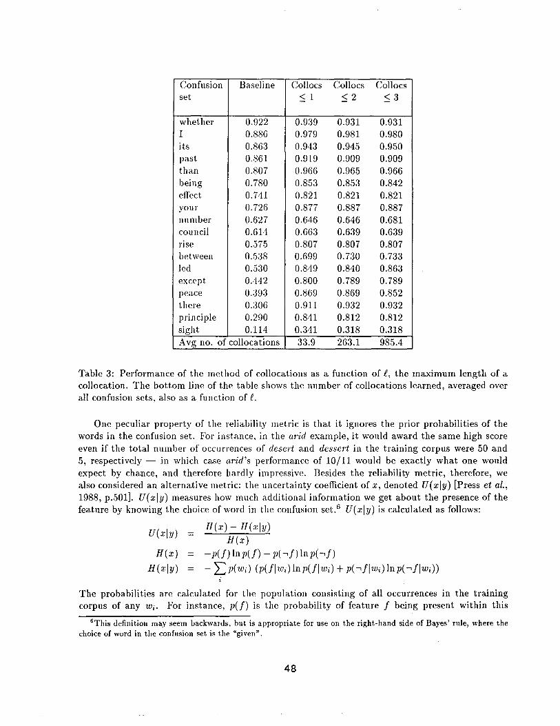
Confllsion set

whether I its past than being effect your number council rise between led except peace there principle sight

Baseline

0.922 0.886 0.863 0.861 0.807 0.780 0.741 0.726 0.627 0.614 0.575 0.538 0.530 0.442 0.393 0.306 0.290 0.114

Collocs Collocs Collocs < 1 _<2 _<3

0.939 0.931 0.931 0.979 0.981 0.980 0.943 0.945 0.950 0.919 0.909 0.909 0.966 0.965 0.966 0.853 0.853 0.842 0.821 0.821 0.821 0.877 0.887 0.887 0.646 0.646 0.681 0.663 0.639 0.639 0.807 0.807 0.807 0.699 0.730 0.733 0.849 0.840 0.863 0.800 0.789 0.789 0.869 0.869 0.852 0.911 0.932 0.932 0.841 0.812 0.812 0.341 0.318 0.318

Avg no. of collocations 33.9 263.1 985.4

Table 3: Performance of the method of collocations as a function of g, the maximum length of a collocation. The bo t tom line of the table shows the number of collocations learned, averaged over all confusion sets, also as a function of e.

One peculiar property of the reliability metric is that it ignores the prior probabilit ies of the words in the confusion set. For instance, in the arid example, it would award the same high score even if the total number of occurrences of desert and dessert in the training corpus were 50 and 5, respectively - - in which case arid's 1)erformance of 10/11 would be exactly what one would expect by chance, and therefore hardly impressive. Besides the reliability metric, therefore, we also considered an alternative metric: the uncertainty coefficient of x, denoted U(xIy ) [Press et al., 1988, p.501]. U(xly ) measures how much additional information we get about the presence of the feature by knowing the choice of word in the confusion set. 6 U(xly ) is calculated as follows:

H ( x ) - H(xly ) v ( x l y ) =

H(x) H(x) = -p ( f ) l n p ( f ) - p(~f)lnp(-~/)

H(xly ) = - ~ p(wl) (p(flwi) lnp(flwl) + p(~flwi) ln p(~flwi) ) i

The probM)ilities are calculated for the population consisting of all occurrences in the training corpus of any wi. For instance, p(f) is the probabil i ty of feature f being present within this

6This definition may seem backwards, but is appropriate for use on the right-hand side of Bayes' rule, where the choice of word in the confusion set is the "given".

4 8

C o n t e x t word peace piece corps peace

un i ted na t ions

ou r hea r t

jus t ice s t a t e

amer i can

aid i n t e r n a t i o n a l

women

war

world piece

over m u s t

g rea t

under

how

t w o

for

a b o u t every

l i t t le

long

o n e

the s o

49 1 41 1

20 0

15 0

27 1

12 0

12 0

12 0

11 0

11 0

11 0

10 0

20 1

40 3 1 15

1 14

11 1

11 1

10 1

10 1

5 12

83 38

4 9

4 9

5 10

6 11

14 23

179 113

9 14

16 22

Tota l occur rences 184 126

Col loca t ion

w corps

D E T w corps

A D V _ _ corps

the __ corps

__ and _ _ of NS

the __ NS

a _ _ P R E P

P R E P _ _ o f

a _ _ o f

f o r

and NS

D E T _ _ N P

NS __ of __ corps NS

P R E P _ _ C O N J

the __ NP

V C O N J

- - NS P U N C

o f v

C, O N J A D J

the NS __

N S A D J

A D V NS _ _

P R E P N S

A D V _ _ P R E P

A D J A D J

N S

A D J

NS N S

peace 47

32

28 27

22

2

37

1

1

1

16

16

32

2 14

14

27

13

13

1

piece 0 0 0 0 0

60 1

35 34

34

0

0 1

45

0

0 1

0

0

25

4 9 4 9

13 26

12 23

17 31

12 22

9 14

62 79

46 54

29 32

To ta l occur rences 184 126

Tab le 4: E x c e r p t s f rom the list of 43 con tex t

words lea rned for {peace, piece} with k = 24.

Each line gives a con tex t word, and the num-

ber of peace and piece occur rences for which

t h a t con tex t word occur red within ± k words.

T h e las t line of the t ab le gives the to ta l num-

ber of occur rences of peace and piece in the

t r a in ing corpus .

Tab le 5: E x c e r p t s f rom the sor ted list of

98 col loca t ions lea rned for {peace, piece} with = 2. Each line gives a co l loca t ion , and

the n u m b e r of peace and piece occur rences it

ma t ched . T h e las t line of the t ab le gives the

to t a l n u m b e r of occur rences of peace and piece in the t r a in ing corpus .

4 9

population. Applying tim U(x]y) metric to the arid example, the value returned now depends on the number of occurrences of desert and dessert in the training corpus. If these numbers are 50 and 5, then U(xly ) = 0.0, reflecting the mfinformativeness of the arid feature in this situation. If instead the numbers are 50 and 500, then U(xly ) = 0.402, indicating arid's better- than-chance ability to pick out desert (10 out of 50 occurrences) over dessert (1 out of 500 occurrences).

To compare the two strength metrics, we tried both on some practice confusion sets. Sometimes one metric did sul)stantially better , sometimes the other. In the balance, the reliability metric seemed to give higher performance. This metric is therefore the one that will be used from here on. It was also used for all experiments involving the method of collocations.

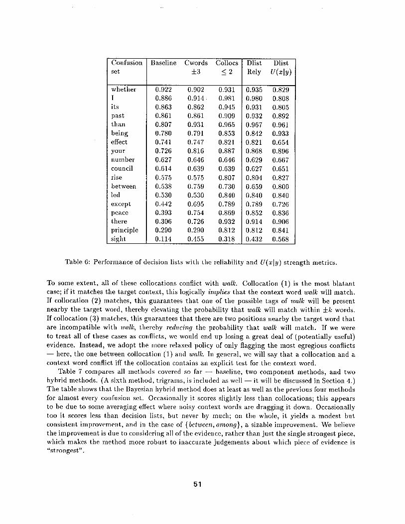
Table 6 shows the performance of decision lists with each metric for the usual confusion sets. As with the practice confusion sets, we see sometimes dramatic performance differences between the two metrics, and no clear winner. For instance, for {I, me}, the reliability metric did bet ter than U(xly) (0.980 versus 0.808); whereas for {between, among}, it did worse (0.659 versus 0.800). Further research is needed to understand the circumstances under which each metric performs best.

Focusing for now on the reliability metric, Table 6 shows that the method of decision lists does, by and large, accomplish what it set out to do - - namely, outperform either component method alone. There axe, however, a few cases where it falls short; for instance, for {between, among}, decision lists score only 0.659, compared with 0.759 for context words and 0.730 for collocations. 7 We believe that the problem lies in the strength metric: because decision lists make their judgements based on a single piece of evidence, their performance is very sensitive to the metric used to select that piece of evidence. But as the relial)ility and U(x[y) metrics indicate, it is not completely clear how the metric should be defined. This problem is addressed in the next section.

3 .5 H y b r i d m e t h o d 2: B a y e s i a n c l a s s i f i e r s

The previous section confirmed that decision lists are effective at combining two complementary methods - - context words and collocations. In doing the combination, however, decision lists look only at the single strongest piece of evidence for a given problem. We hypothesize that even bet ter performance can be obtained by ta.king into account all available evidence. This section presents a method of doing this based on Bayesian classifiers.

Like decision lists, the Bayesian method starts with a list of all features, sorted by decreasing strength. It classifies a.n ambiguous target word by matching each feature in the list in turn against the target context. Instead of stopping at the first matching feature, however, it traverses the entire list, combining evidence fi'om all matching features, and resolving conflicts where necessary.

This method is essentially the same as the one for collocations (see Figure 2), except that it uses context words as well as collocations for the features. The only new wrinkle is in checking for conflicts between features (in step (2) a.t run tilne), as there are now two kinds of features to consider. If both features are context words, we say the features never conflict (as in the method of context words). If both features are collocations, we say they conflict iff they overlap (as in the method of collocations). The new case is if one feature is a context word, and the other is a collocation. Consider, for example, the context word walk, and the following collocations:

(1) __ walk ( 2 ) _ v

(3) CONJ __ P R E P

7If we use the U(x[y) met r ic ins tead , then decision lists fall down on different examples ; e.g., {its, it 's}.

50

Confusion se t

whether I its past than being effect your number council rise between led except peace there principle sight

Baseline Cwords Collocs :53 < 2

0.922 0.902 0.931 0.886 0.914 0.981 0.863 0.862 0.945 0.861 0.861 0.909 0.807 0.931 0.965 0.780 0.791 0.853 0.741 0.747 0.821 0.726 0.816 0.887 0.627 0.646 0.646 0.614 0.639 0.639 0.575 0.575 0.807 0.538 0.759 0.730 0.530 0.530 0.840 0.442 0.695 0.789 0.393 0.754 0.869 0.306 0.726 0.932 0.290 0.290 0.812 0.114 0.455 0.318

Dlist Dlist Rely U(xly )

0.935 0.829 0.980 0.808 0.931 0.805 0.932 0.892 0.967 0.961 0.842 0.933 0.821 0.654 0.868 0.896 0.629 0.667 0.627 0.651 0.804 0.827 0.659 0.800 0.840 0.840 0.789 0.726 0.852 0.836 0.914 0.906 0.812 0.841 0.432 0.568

Table 6: Performance of decision lists with the reliability and U(xly ) strength metrics.

To some extent, all of these collocations conflict with walk. Collocation (1) is the most blatant case; if it matches the target context, this logically implies that the context word walk will match. If collocation (2) matches, this guarantees that one of the possible tags of walk will be present nearby the target word, thereby elevating the probabili ty that walk will match within :5k words. If collocation (3) matches, this guarantees that there are two positions nearby the target word that are incompatible with walk, thereby reducing the probabili ty that walk will match. If we were to treat all of these cases as conflicts, we would end up losing a great deal of (potentially useful) evidence. Instead, we adopt the more relaxed policy of only flagging the most egregious conflicts - - here, the one between collocation (1) and walk. In general, we will say that a collocation and a context word conflict iff the collocation contains an explicit test for the context word.

Table 7 compares all methods covered so far - - baseline, two component methods, and two hybrid methods. (A sixth method, trigrams, is included as well - - it will be discussed in Section 4.) The table shows that the Bayesian hyt)rid method does at least as well as the previous four methods for almost every confusion set. Occasionally it scores slightly less than collocations; this appears to be due to some averaging effect where noisy context words are dragging it down. Occasionally too it scores less than decision lists, 1)ut never by much; on the whole, it yields a modest but consistent improvement, and in the case of {between, among}, a sizable improvement. We believe the improvement is due to considering all of the evidence, rather than just the single strongest piece, which makes the method more robust to inaccurate judgements about which piece of evidence is "strongest".

51

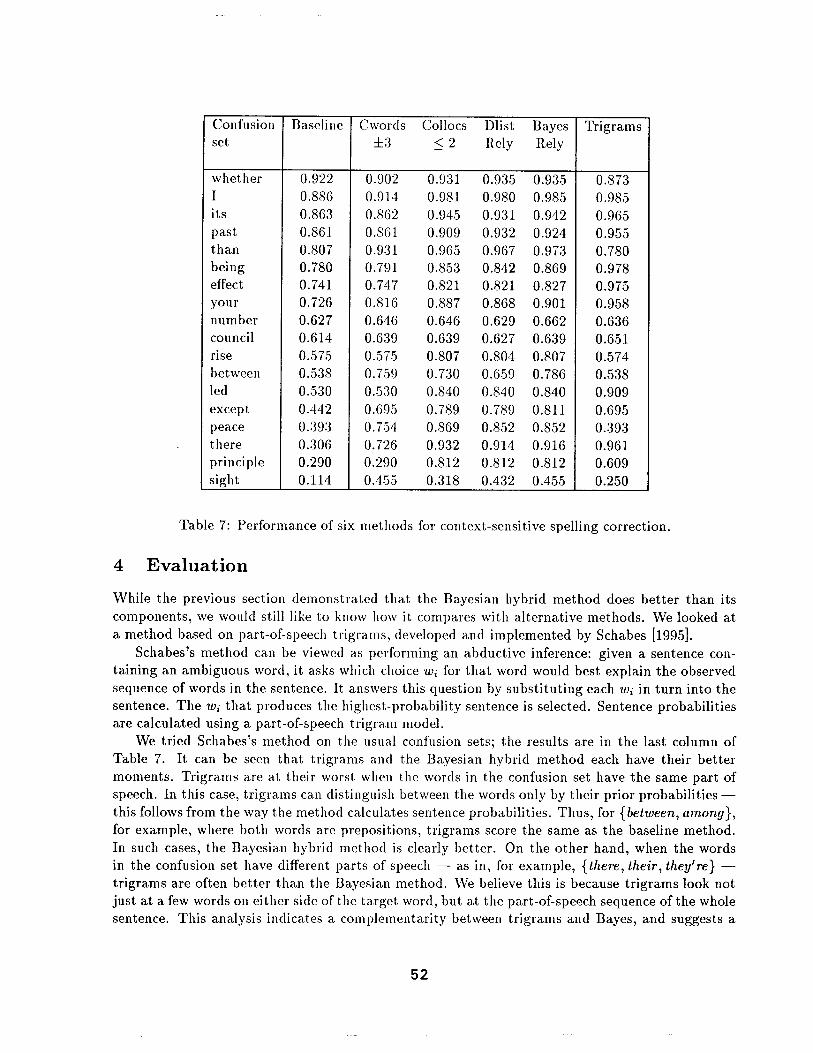
Confusion set

whether I its past than being effect your number council rise between led except peace there principle sight

Baseline

0.922 0.886 0.863 0.861 0.807 0.780 0.741 0.726 0.627 0.614 O.575 0.538 0.530 0.442 0.393 0.306 0.290 0.114

Cwords Collocs Dlist Bayes :t:3 _< 2 Rely Rely

0.902 0.931 0.935 0.935 0.914 0.981 0.980 0.985 0.862 0.945 0.931 0.942 0.861 0.909 0.932 0.924 0.931 0.965 0.967 0.973 0.791 0.853 0.842 0.869 0.747 0.821 0.821 0.827 0.816 0.887 0.868 0.901 0.646 0.646 0.629 0.662 0.639 0.639 0.627 0.639 0.575 0.807 0.804 0.807 0.759 0.730 0.659 0.786 0.530 0.840 0.840 0.840 0.695 0.789 0.789 0.811 0.754 0.869 0.852 0.852 0.726 0.932 0.914 0.916 0.290 0.812 0.812 0.812 0.455 0.318 0.432 0.455

Trigrams

0.873 0.985 0.965 0.955 0.780 0.978 0.975 0.958 0.636 0.651 0.574 0.538 0.909 0.695 0.393 0.961 0.609 0.250

Table 7: Performance of six methods for context-sensitive spelling correction.

4 E v a l u a t i o n

While the previous section demonstrated that the Bayesian hybrid method does bet ter than its components, we would still like to know how it compares with alternative methods. We looked at a method based on part-of-speech trigrams, developed and implemented by Schabes [1995].

Schabes's method can be viewed as performing an abductive inference: given a sentence con- taining an ambiguous word, it asks which choice wi for that word would best explain the observed sequence of words in the sentence. It answers this question by subst i tut ing each wi in turn into the sentence. The wi that produces the highest-probabili ty sentence is selected. Sentence probabilit ies are calculated using a part-of-speech trigram model.

We tried Schabes's method on the usual confusion sets; the results are in the last column of Table 7. It can be seen that trigrams and the Bayesian hybrid method each have their bet ter moments. Trigrams are at their worst when the words in the confusion set have the same part of speech. In this case, trigrams can distinguish between the words only by their prior probabilit ies - - this follows from the way the method calculates sentence probabilities. Thus, for {between, among}, for example, where both words are prepositions, trigrams score the same as the baseline method. In such cases, the Bayesian hybrid method is clearly better . On the other hand, when the words in the confusion set have different parts of speech - - as in, for example, {there, their, they%e} - - trigrams are often bet ter than the Bayesian method. We believe this is because tr igrams look not just at a few words on either side of the target word, but at the part-of-speech sequence of the whole sentence. This analysis indicates a complementari ty between trigrams and Bayes, and suggests a

5 2

combination ill which trigrams would be applied first, but if trigrams determine that the words in the confusion set have the same part of speech for the sentence at issue, then the sentence would be passed to the Bayesian method. This is a research direction we plan to pursue.

5 Conc lus ion

The work reported here builds on Yarowsky's use of decision lists to combine two component methods - - context words and collocations. Decision lists pool the evidence fl'om the two methods, and solve a target problem by applying the single strongest piece of evidence, whichever type that happens to be. This paper investigated the hypothesis that even better performance can be obtained by basing decisions on not just the single strongest piece of evidence, but on M1 available evidence. A method for doing this, based on Bayesian classifiers, was presented. It was applied to the task of context-sensitive spelling correction, and was found to outperform the component methods as well as decision lists. A comparison of the Bayesian hybrid method with Schabes's trigram-based method suggested a further combination in which trigrams would be used when the words in the confusion set had different parts of speech, and the Bayesian method would be used otherwise. This is a direction we plan to pursue in future research.

A c k n o w l e d g e m e n t s

We would like to thank Bill Freeman, Yves Schabes, Emmanuel Roche, and Jacki Golding for helpful and enjoyable discussions on the work reported here.

References

Joseph L. Fleiss. Statistical Methods for Rates and Proportions. John Wiley and Sons, 1981.

Stuart Berg Flexner, editor. Random House Unabridged Dictionary. Random House, New York, 1983. Second edition.

William A. Gale, Kenneth W. Church, and David Yarowsky. Discrimination decisions for 100,000- dimensional spaces. In Current Issues in Computational Linguistics: In Honour off Don Walker, pages 429-450. Kluwer Academic Publishers, 1994.

H. Ku~era and W. N. Francis. Computational Analysis of Present-Day American English. Brown University Press, Providence, RI, 1967.

Mitchell P. Marcus, Beatrice Santorini, and Mary Ann Marcinkiewicz. Building a large annotated corpus of English: The Penn Treebank. Computational Linguistics, 19(2):313-330, June 1993.

Eric Mays, Fred J. Damerau, and Robert L. Mercer. Context based spelling correction. Information Processing ~4 Management, 27(5):517-522, 1991.

William Press, Brian Flannery, Saul Teukolsky, and William Vetterling. Numerical Recipes in C: The Art of Scientific Computing. Cambridge University Press, New York, 1988. Reprinted twice.

Yves Schabes. Technical report, Mitsubishi Electric Research Laboratories, 1995. Forthcoming.

David Yarowsky. A comparison of corpus-based techniques for restoring accents in Spanish and French text. In Proceedings of the 2nd Annual Workshop on Very Large Corpora, Kyoto, 1994.

53