A Bayesian approach to feed reconstruction

A Bayesian approach to feed reconstruction

by

Naveen Kartik Conjeevaram Krishnakumar

B.Tech Chemical Engineering, Indian Institute of Technology, Madras

(2011)

Submitted to the School of Engineering

in partial fulfillment of the requirements for the degree of

Master of Science in Computation for Design and Optimization

at the

MASSACHUSETTS INSTITUTE OF TECHNOLOGY

June 2013

@ Massachusetts Institute of Technology 2013. All rights res

2,PAI E S1

arCHNES

A uthor .........................School of Engineering

May 23, 2013

Certified by..... ..................... ....................................

Youssef M. MarzoukAssociate Professor of Aeronautics and Astronautics

Thesis Supervisor

A ccepted by ................................... ........Ni H stantinou

Co-Director, Computation for Desigd and Optimization

A Bayesian approach to feed reconstruction

by

Naveen Kartik Conjeevaram Krishnakumar

Submitted to the School of Engineeringon May 23, 2013, in partial fulfillment of the

requirements for the degree ofMaster of Science in Computation for Design and Optimization

Abstract

In this thesis, we developed a Bayesian approach to estimate the detailed compositionof an unknown feedstock in a chemical plant by combining information from a fewbulk measurements of the feedstock in the plant along with some detailed compositioninformation of a similar feedstock that was measured in a laboratory. The complexityof the Bayesian model combined with the simplex-type constraints on the weightfractions makes it difficult to sample from the resulting high-dimensional posteriordistribution. We reviewed and implemented different algorithms to generate samplesfrom this posterior that satisfy the given constraints. We tested our approach on adata set from a plant.

Thesis Supervisor: Youssef M. MarzoukTitle: Associate Professor of Aeronautics and Astronautics

3

Acknowledgments

First off, I would like to acknowledge my parents Gowri and Krishnakumar, to whom

I owe all my past, present and future success. Their unconditional love and support

enabled me to pursue my dreams and desires, and become the person I am today.

I would also like to thank my advisor Professor Youssef Marzouk, who shaped my

journey through MIT. He is intelligent, inspirational, and most of all, the best friend

a student could ask for. I could fill this entire page, and still not convey the deep

sense of gratitude that I feel today. However, a simple thank you will have to suffice

for now. I would like to thank the members of the ACDL community and the UQ

lab, for being amazing friends, co-workers and labmates. In particular, I would like

to thank Alessio Spantini, who endured many a sleepless night solving problem sets

and assignments with me, and Tiangang Cui, who would always patiently listen to

my research ramblings.

I would also like to thank my all my friends, both in and outside Boston, who

helped me helped me maintain my sanity through the crazy times at MIT. Finally, I

would like to thank Barbara Lechner, our program administrator, who passed away

recently. She was a truly warm and kind person, who would put the needs of students

before herself. We will all miss her wonderful smile.

I would also like to acknowledge BP for supporting this research, and thank Randy

Field for his help through the project.

5

Contents

1 Introduction

1.1 Feed reconstruction in chemical processes . . . . . . . . .

1.2 Pseudo-compound framework . . . . . . . . . . . . . . .

1.3 Current approaches to feed reconstruction . . . . . . . .

1.3.1 Drawbacks of current feed reconstruction schemes

1.4 Bayesian inference . . . . . . . . . . . . . . . . . . . . .

1.5 Research objectives . . . . . . . . . . . . . . . . . . . . .

1.6 Thesis outline . . . . . . . . . . . . . . . . . . . . . . . .

2 A Bayesian inference approach to feed reconstruction

2.1 Available data . . . . . . . . . . . . . . . . . . . . . . . .

2.1.1 Laboratory data . . . . . . . . . . . . . . . . . . .

2.1.2 Plant data . . . . . . . . . . . . . . . . . . . . . .

2.2 Bayesian formulation of feed reconstruction . . . . . . . .

2.2.1 Target variable . . . . . . . . . . . . . . . . . . .

2.2.2 Prior distribution . . . . . . . . . . . . . . . . . .

2.2.3 Likelihood . . . . . . . . . . . . . . . . . . . . . .

2.2.4 Posterior distribution . . . . . . . . . . . . . . . .

2.3 Advantages of the Bayesian approach . . . . . . . . . . .

2.4 Exploring the posterior distribution . . . . . . . . . . . .

3 Computational aspects of feed reconstruction

3.1 Introduction.............. ....... ..... .

7

13

13

14

15

16

18

19

19

21

. . . . . . . 22

. . . . . . . 22

. . . . . . . 23

. . . . . . . 23

. . . . . . . 23

. . . . . . . 25

. . . . . . . 31

. . . . . . . 32

. . . . . . . 34

. . . . . . . 34

37

37

3.1.1 Monte Carlo methods . . . . . . .

3.2 Numerical integration using Monte Carlo

3.3 Markov chain Monte Carlo . . . . . . . .

3.3.1 Literature Review . . . . . . . . .

3.3.2 Sampling problem . . . . . . . . .

3.3.3 Gibbs sampler . . . . . . . . . . .

3.3.4 Hit-and-run sampler . . . . . . .

3.3.5 Directional independence sampler

3.4 Summary . . . . . . . . . . . . . . . . .

sampling

4 Results

4.1 Low dimensional examples . . . . . . . . . . . . . . . . . . . . . . . .

4.1.1 Gibbs sampler . . . . . . . . . . . . . . . . . . . . . . . . . . .

4.1.2 Hit-and-run sampler . . . . . . . . . . . . . . . . . . . . . . .

4.1.3 Directional independence sampler . . . . . . . . . . . . . . . .

4.2 Feed reconstruction example . . . . . . . . . . . . . . . . . . . . . . .

4.3 Sum m ary . . . . . . . . . . . . . . . . . . . . . . . . . . . . . . . . .

5 Conclusions

5.1 Future work . . . . . . . . . . . . . . . . . . . . . . . . . . . . . . . .

A Fully Bayesian procedure

B Restriction of a Gaussian to a line

C Projected Normal Distribution

8

38

39

40

40

41

43

45

48

55

57

57

59

61

63

65

69

71

72

75

77

79

List of Figures

2-1 Feed reconstruction framework used to develop Bayesian model . . . 22

2-2 Grid of inference target weight fractions . . . . . . . . . . . . . . . . 24

2-3 A schematic illustrating the "straddling" issue with assigning prior

means, with a section for the matrix Y . . . . . . . . . . . . . . . . . 26

2-4 A schematic illustrating the prior parameter estimation procedure . 30

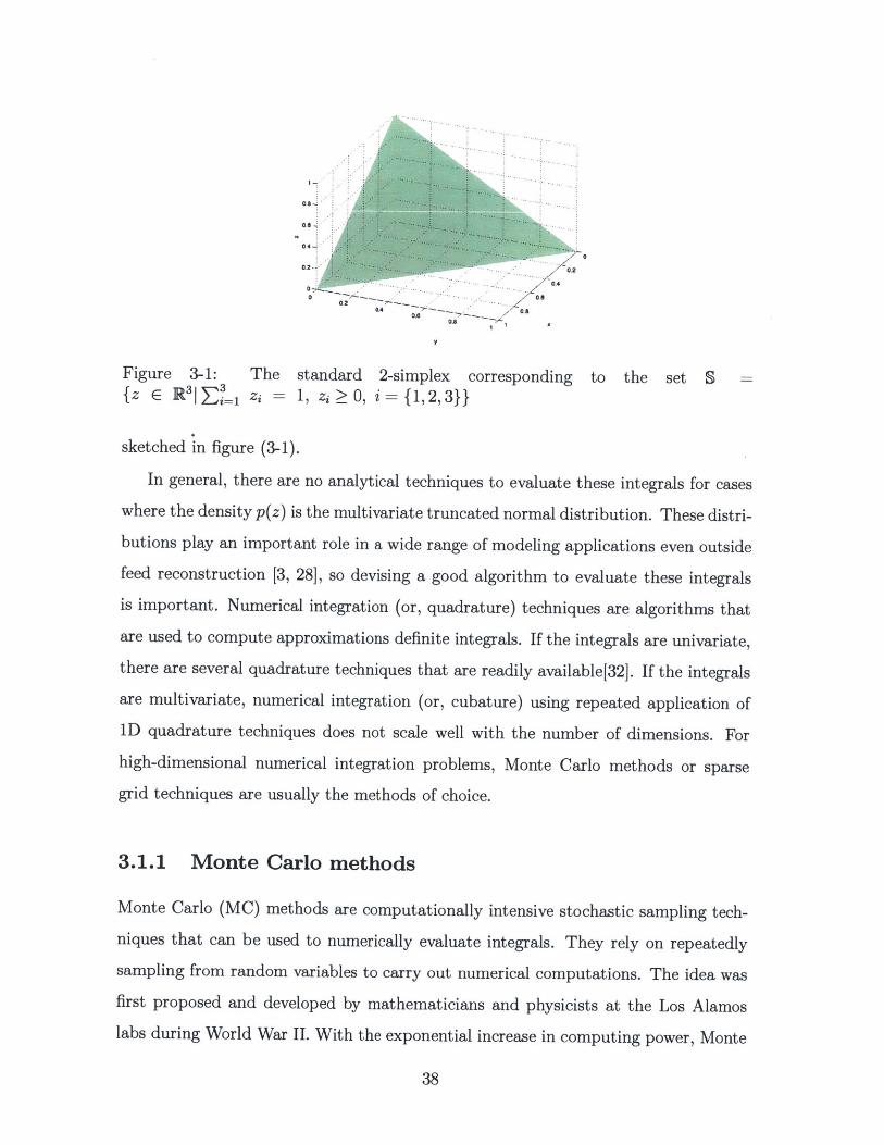
3-1 The standard 2-simplex corresponding to the set S {z E R3 zj = 1, z >

0, i = { 1, 2,3}} . . . . . . . . . . . . . . . . . . . . . . . . . . . . . . 38

3-2 Visual Representation of the Hit-and-Run algorithm. Image Courtesy:

[20] . . . . . . . . . . . . . . . . . . . . . . . . . . . . . . . . . . . . 45

4-1 Case 1: Scatter plot of samples generated by the Gibbs sampling algo-

rithm, along with the sample trace and autocorrelation plots ..... 59


rithm, along with the sample trace and autocorrelation plots . . . . . 59


rithm, along with the sample trace and autocorrelation plots . . . . . 60

4-4 Case 1: Scatter plot of samples generated by the hit-and-run sampling

algorithm, along with the sample trace and autocorrelation plots . . . 61





9

4-7 Case 1: Scatter plot of samples generated by the directional indepen-

dence sampler, along with the sample trace and autocorrelation plots 63





4-10 Sample trace and autocorrelations along selected coordinates in the

Bayesian feed reconstruction example . . . . . . . . . . . . . . . . . . 66

4-11 Marginal densities of samples generated from Bayesian posterior dis-

tribution for 2 different families of pseudo-compounds . . . . . . . . . 67

4-12 Marginal densities of concentrations of pseudo-compounds in a partic-

ular family for varying bulk concentrations . . . . . . . . . . . . . . . 68

4-13 Comparing marginal densities of concentrations of pseudo-compounds

in a particular family for varying degrees-of-belief in the bulk and lab-

oratory measurements respectively . . . . . . . . . . . . . . . . . . . 68

C-1 Plots observed samples for different values of IIp, with the population

mean direction highlighted in red . . . . . . . . . . . . . . . . . . . . 81

10

List of Tables

4.1 Comparing the mean of the truncated normal distribution calculated

using 2-D quadrature and the sample mean for the Gibbs sampler . . 60


using 2-D quadrature and the sample mean for the hit-and-run sampler 62


using 2-D quadrature and the sample mean for the directional inde-

pendence sampler . . . . . . . . . . . . . . . . . . . . . . . . . . . . . 64

11

Chapter 1

Introduction

1.1 Feed reconstruction in chemical processes

In chemical plants and oil refineries, the typical process stream contains a mixture of a

large number of molecular species. In oil refineries for example, it is not uncommon to

observe streams with several thousand hydrocarbon species [19]. When these streams

are used as a feed to reactors or unit operations in the plant, the detailed composition

of the stream becomes important. Accurate knowledge of the stream composition in

terms of the molecular constituents allows us to build good operating models (such

as kinetic models), which in turn can be used control the reactor conditions, prod-

uct yield and quality. Recent advances in analytical chemistry techniques (such as

conventional gas chromatography (1D-GC) and comprehensive two-dimensional gas

chromatography (GC x GC) [35]) allow us to to obtain detailed molecular composi-

tions of various streams. However, these techniques are expensive, time consuming

and rarely done in-plant. This means that it is not possible to analytically obtain the

detailed composition of various streams in the plant on a regular basis. However, the

dynamic nature of the modern refinery or chemical plant results in a changing stream

composition on a daily, if not hourly, basis. To overcome this difficulty, it is common

practice to resort to feed reconstruction techniques.

Feed reconstruction or composition modeling techniques are a class of algorithms

that are used to estimate the detailed composition of a mixture starting from a limited

13

number of bulk property measurements (such as average molar mass, distillation

data, specific density, atomic concentrations, etc.) [34]. In the absence of detailed

experimental measurements, feed reconstruction algorithms provide a rapid way to

obtain detailed composition data. These techniques have become increasingly popular

with the rise of cheap computational power and the high cost of analytical techniques.

To handle the sheer number of molecular components that are present in a typical

feed, it is common practice to represent groups of molecules with a single represen-

tative molecule called a pseudo-compound [19]. This procedure is also employed in

analyzing the kinetics of complex mixtures of molecules, and is sometimes referred to

as a lumping approach [22]. The pseudo-compound framework allows us to represent

the stream with a significantly smaller set of species. However, it is still diffucult to

experimentally ascertain the exact concentrations of these pseudo-compounds. We

shall first elaborate on the pseudo- compound/lumping framework that we utilize

here before we describe the general feed reconstruction process.

1.2 Pseudo-compound framework

The pseudo-compounds that are chosen to represent a particular feedstock must be

sufficiently representative of the underlying actual molecular species to minimize any

resulting lumping errors. In an oil refining context, the large number of hydrocarbons

that that constitute any typical feed stream allow for a variety of pseudo-compound

representations.

One popular choice of pseudo-compounds [19, 29, 35, 46] is based on identifying

chemical families, which may be based on certain parameters, such as structural or

reactive attributes. Once the chemical families are identified, the pseudo-compounds

are then generated by choosing different carbon number homologues corresponding

to each chemical family. For instance, if we identify the Thiophene family (molecules

that contain at least one thiophene ring) as one possible constituent of our feedstock,

then we may choose C1-Thiophene, C3-Thiophene and C7-Thiophene as pseudo-

compounds to represent all members of the Thiophene family in the feedstock. The

14

chemical families that are identified often depend on the feedstock in question. Ana-

lytical techniques can be used to understand the molecular composition of the feed-

stock and reveal the types of chemical families that are required to model it. In Gas

Oil feeds, for example, experimental analyses have been used to define 28 different

chemical families that can be processed in a refinery [19], while a larger number of

such families have been used to model vacuum gas oil cuts [46].

The carbon numbers corresponding to homologues of the chemical families are

chosen based on the boiling range of the feedstock. Gas oil, which has a low boiling

range, is typically composed of low carbon number molecules, while high boiling feeds

such as vacuum gas oil require a higher carbon number range to model accurately.

This approach to feed modeling, which assumes that the given mixture of com-

pounds can be described by a fixed library of pseudo-compounds , is said to be a

deterministic representation of the feed. Stochastic representations, on the other

hand, do not rely on a fixed library of pseudo-compounds. Instead, they rely on

a distribution of molecular attributes and sample from this distribution to generate

a realization of pseudo-compounds [29, 46]. However, stochastic methods are usu-

ally difficult to implement because they are computationally intensive and rely on

distribution information that is usually hard to obtain [50].

Ultimately, the choice of pseudo-compounds depends on the purpose and the de-

sired accuracy of the modeling exercise. For low-fidelity models, it may be sufficient

to pick a few chemical families and carbon number homologues. State of the art

modeling [35, 34, 50, 27] techniques rely on generating a large number of chemical

families by varying structural attributes and then using finely discretized carbon num-

ber ranges. The modeler has to choose the pseudo-compounds appropriately, so as to

reduce error in the estimation of any variables of interest.

1.3 Current approaches to feed reconstruction

Liguras and Allen [23] proposed one of the first feed reconstruction algorithms, which

was based on minimizing a weighted objective function based on bulk measurements

15

collected using NMR spectroscopy. Their method was innovative, but it required a

large number of property measurements to be effective. Since then, several different

feed reconstruction techniques have been proposed.

Typical modern modeling techniques involve minimizing a specific function of de-

viation of the observed bulk measurements from the calculated bulk measurements by

varying the concentrations of the pseudo-compounds that are assumed to constitute

the feed. Androulakis et al. [4] used a constrained weighted least squares approach

to modeling the composition of diesel fuel. Van Geem et al. [45] proposed a feed

reconstruction scheme that characterizes a given feedstock by maximizing a criterion

similar to Shannon's entropy. Quanne and Jaffe propose a similar method, where

the pseudo-compounds are replaced by vectors called Structured Oriented Lumping

(SOL) vectors. These methods assume that the feedstock being modeled can be

completely described by the fixed library of pseudo-compounds.

Alternative approaches to feed reconstruction have focused on coupling the mini-

mization step with stochastic representation of the feed [29]. The pseudo-compounds

are first generated using a Monte Carlo routine, and then their concentrations are

calculated so that the computed bulk properties match the experimental measure-

ments. Trauth et al. [44] used this method to model the composition of petroleum

resid, while Verstraete et al. [46] adopted a similar idea to model vacuum gas oils. To

reduce the computational burden associated with stochastic models, Campbell et al.

[9] used a Monte Carlo generation method coupled with a quadrature technique to

work with a reduced basis of pseudo-compounds. Pyl et al. [34] proposed a stochastic

composition modeling technique that uses constrained homologous series and empir-

ically verified structural distributions to greatly reduce the number of unknowns in

the optimization step.

1.3.1 Drawbacks of current feed reconstruction schemes

While feed reconstruction schemes have been around for quite some time, they all

suffer from similar drawbacks. The deterministic approaches to feed reconstruction

sometimes require bulk properties that are hard to obtain, while the stochastic ap-

16

proaches rely on attribute distribution information that is mostly fixed on an ad-hoc

or empirical basis.

In typical composition modeling techniques, it is difficult to add any new measure-

ment information in a systematic manner. For example, if a modeler wishes to add a

new type of bulk measurement to increase the accuracy of the predicted composition,

it is not immediately obvious how one may modify the algorithm to incorporate this

new piece of information. In particular, if we have any past detailed measurements

that could improve current concentration estimates, we cannot take advantage of this

information without significantly modifying the algorithm.

Furthermore, traditional composition modeling techniques do not incorporate a

systematic idea of uncertainty in the reconstruction process. Understanding uncer-

tainty in the composition of any feed stream in a chemical plant/refinery is very

important. The uncertainty in the concentration of any pseudo-compounds of inter-

est allows us to understand the impact of variation of bulk properties on the feed

composition. Furthermore, the output of the feed reconstruction process might be

used to model downstream unit operations like chemical reactors. In that case, hav-

ing a handle on the input uncertainty to a unit operation gives us an idea of the

resulting output uncertainty of the process. This becomes particularly important in

applications such as oil refining, where the final product is expected to conform to

certain quality standards. Having a low output uncertainty ensures that the quality

of the product remains consistent across time.

Finally, from an experimental design point of view, an accurate quantification of

uncertainty in the feed reconstruction process would allow us to analyze if we can

reduce the uncertainty in any particular quantities of interest by incorporating addi-

tional experimental measurements. For example, environmental regulations require

a strict control on the level of sulphur in diesel produced in oil refineries. Therefore,

it is important to estimate the composition of sulphur-containing psuedo-compounds

with a high degree of confidence. However, it may only be possible to obtain a small

number of bulk measurements. If we can quantify the uncertainty in the feed recon-

struction, it is possible to implement an experimental design procedure to choose the

17

bulk measurements that yield the lowest level of uncertainty (or inversely, the high-

est degree of confidence) in the concentrations of interest. The drawbacks that we

have outlined in this section motivate the construction of a new feed reconstruction

approach, by adopting a Bayesian approach to the problem.

1.4 Bayesian inference

Parametric inference is the branch of statistical inference that is concerned with iden-

tifying parameters of a model given noisy data that is assumed to be generated from

the same model. Traditional parameter inference frameworks (sometimes referred to

as frequentist inference) assume that the parameters in a model are constant and

any deviation in measurement from the model prediction is attributed to noise [48].

Typical frequentist inference techniques focus on finding a best estimate for each pa-

rameter (also called a point estimate), along with an associated confidence interval.

The Bayesian approach to statistics is motivated by the simple idea that a prob-

ability value assigned to an event represents a degree of belief, rather than a limiting

frequency of the event. We can extend this notion of "probability as a degree-of-belief'

to inference using Bayesian statistics. Contrary to frequentist inference, Bayesian in-

ference assumes that the underlying model parameters are random variables. Bayesian

parametric inference computes a probability distribution for each unknown param-

eter from the data. Subsequent point estimates and confidence intervals are then

calculated from the probability distributions.

Since the Bayesian inference procedure assigns probability distributions to each

parameter, we need to choose a way to update the probability distributions with noisy

data from the model. The most popular updating rule is the Bayes rule [41], which

we shall describe below.

Let us denote the set of parameters as 0. First, we choose a probability distribution

p(9), called a prior, that reflects our beliefs about the parameters before observing

any data (denoted by D). Then, we choose a function C called a likelihood, which

gives the probability of observing V, given 0. Then, by Bayes rule,

18

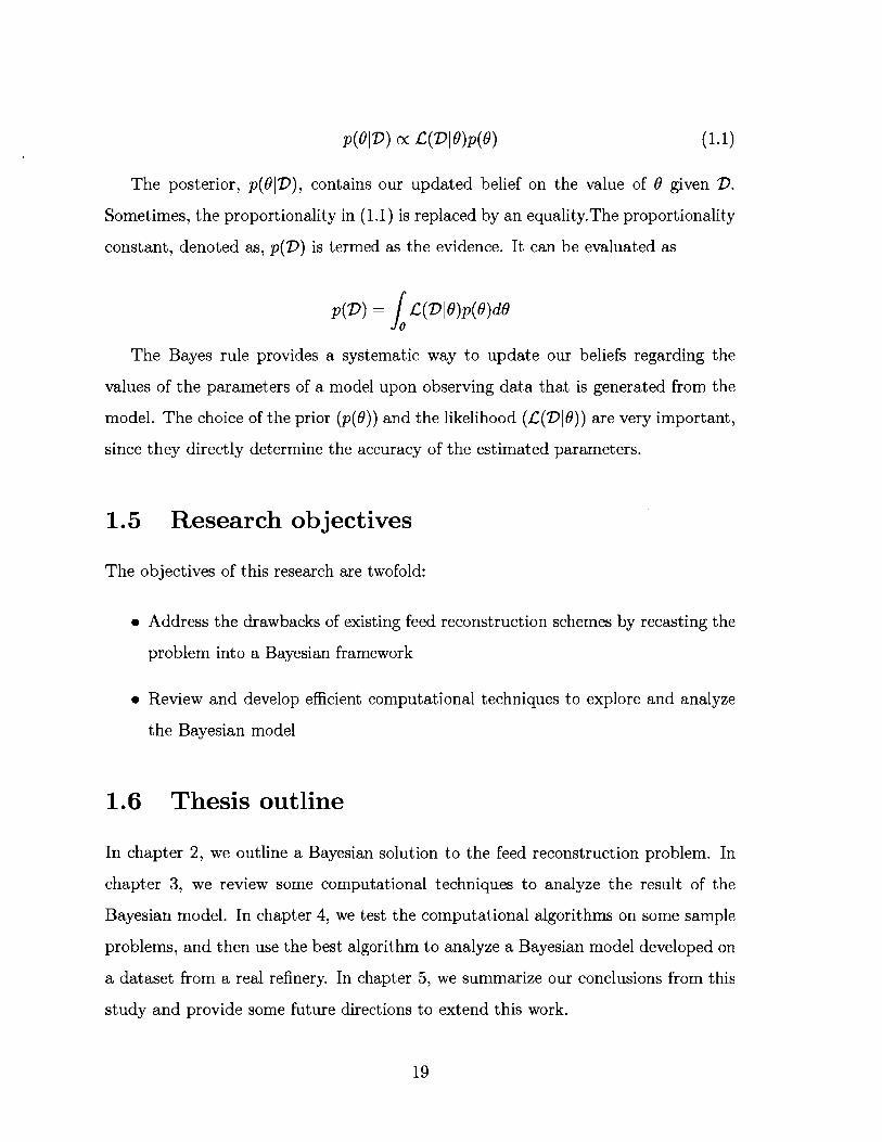
p(6|D) oc L(D|O)p(9) (1.1)

The posterior, p(ID), contains our updated belief on the value of 0 given D.

Sometimes, the proportionality in (1.1) is replaced by an equality.The proportionality

constant, denoted as, p(D) is termed as the evidence. It can be evaluated as

p(D) jL(D|9)p(9)d9

The Bayes rule provides a systematic way to update our beliefs regarding the

values of the parameters of a model upon observing data that is generated from the

model. The choice of the prior (p(9)) and the likelihood (L(D|j)) are very important,

since they directly determine the accuracy of the estimated parameters.

1.5 Research objectives

The objectives of this research are twofold:

* Address the drawbacks of existing feed reconstruction schemes by recasting the

problem into a Bayesian framework

" Review and develop efficient computational techniques to explore and analyze

the Bayesian model

1.6 Thesis outline

In chapter 2, we outline a Bayesian solution to the feed reconstruction problem. In

chapter 3, we review some computational techniques to analyze the result of the

Bayesian model. In chapter 4, we test the computational algorithms on some sample

problems, and then use the best algorithm to analyze a Bayesian model developed on

a dataset from a real refinery. In chapter 5, we summarize our conclusions from this

study and provide some future directions to extend this work.

19

Chapter 2

A Bayesian inference approach to

feed reconstruction

In this chapter, we shall describe a Bayesian approach to the feed reconstruction

problem. While we shall apply this feed reconstruction approach specifically to model

crude fractions in an oil refinery, the general framework can be extended to other

chemical systems.

We are interested in developing a Bayesian model for the following framework: We

have the detailed description for a particular type of feedstock in terms of the cho-

sen pseudo-compounds from analytical chemistry techniques in a laboratory setting.

These experiments are time-consuming and expensive, so we cannot repeat them on

a daily basis in the chemical plant/refinery. Instead, we would like to predict the

detailed composition from properties like distillation curves and bulk concentrations

that can be easily measured in the plant. In this framework, a feed reconstruction

model should combine the detailed information from the laboratory with the bulk

information of the feedstock measured in the plant to infer the detailed composition

of the feedstock in the refinery (in terms of weight percents/fractions). A schematic

representation of this feed reconstruction procedure is presented in figure (2-1).

In the following sections, we shall first explain type of laboratory and plant infor-

mation that we assume is available to the feed reconstruction process. Then, we shall

outline the Bayesian inference procedure and elaborate on the details.

21

Fingerprint Library|

Figure 2-1: Feed reconstruction framework used to develop Bayesian model

2.1 Available data

2.1.1 Laboratory data

Detailed analytical techniques such as two-dimensional gas chromatography allow ex-

perimentalists to identify the concentrations (in weight percent) of individual species

with great precision. By applying these techniques on a sample feedstock (which is

assumed to be representative of any typical feed that you might encounter in the re-

finery), we can first identify a set of pseudo-compounds that can sufficiently describe

the feed along with with their concentrations (in weight fractions) and molecular

weights. The pseudo-compounds themselves are assumed belong to certain families,

while individual pseudo-compounds within each family are differentiated by carbon

number (as described in the previous chapter).

Since each pseudo-compound refers to a collection of molecules, it is not going

to have a single boiling temperature. Instead, each pseudo-compound will boil over

a temperature range. Along with their concentrations, we shall also assume that

we can measure the initial and final boiling point of each pseudo- compound that is

identified1 .

'Since boiling information is a by-product of most detailed analytical techniques, this assumptionis not unjustified

22

2.1.2 Plant data

The Plant Data refers to any bulk measurements of the feed that are collected in the

refinery. While bulk measurements (or assays) could refer to a wide range of physical

properties (such as atomic concentrations, refractive indices, specific gravities etc.),

we assume that any assay that is collected in the refinery includes some distillation

analysis (such as the ASTM D86 distillation [12]). At the simplest level, the resulting

data can be understood as a set of boiling ranges and fraction of the crude that boils

in those corresponding ranges.

These assumptions on data availability that we have made so far might seem

restrictive at first glance. The subsequent analysis however, is general enough to deal

with the absence of any type of information (albeit with slight modifications). We

have chosen this particular structure in our data available since this refers to the most

general type of data that is used as an input to a feed reconstruction procedure.

2.2 Bayesian formulation of feed reconstruction

The first step in constructing a Bayesian model for a given problem is to identify

the parameters in the problem. Once we identify the parameters, we need to assign

a prior distribution on the range of values that the parameters can take. Then, we

need to define a likelihood function on the data that we observe. Finally, we need to

use equation (1.1) to compute the posterior distribution on the parameters. In the

following subsections, we shall construct a Bayesian model for the feed reconstruction

problem using the same outline.

2.2.1 Target variable

Before we begin constructing probability distributions, we must first identify the

parameters that we wish to infer in modeling the composition of any feedstock. First,

we assume that the modeler has the pseudo-compounds of interest from the laboratory

data and the boiling temperature ranges for the feedstock from the plant data. We

23

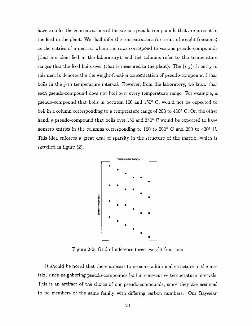
have to infer the concentrations of the various pseudo-compounds that are present in

the feed in the plant. We shall infer the concentrations (in terms of weight fractions)

as the entries of a matrix, where the rows correspond to various pseudo-compounds

(that are identified in the laboratory), and the columns refer to the temperature

ranges that the feed boils over (that is measured in the plant). The (ij)-th entry in

this matrix denotes the the weight-fraction concentration of pseudo-compound i that

boils in the j-th temperature interval. However, from the laboratory, we know that

each pseudo-compound does not boil over every temperature range: For example, a

pseudo-compound that boils in between 100 and 150* C, would not be expected to

boil in a column corresponding to a temperature range of 200 to 4000 C. On the other

hand, a pseudo-compound that boils over 150 and 350* C would be expected to have

nonzero entries in the columns corresponding to 100 to 200* C and 200 to 4000 C.

This idea enforces a great deal of sparsity in the structure of the matrix, which is

sketched in figure (2).

Temperature Ranges

0

*

Figure 2-2: Grid of inference target weight fractions

It should be noted that there appears to be some additional structure in the ma-

trix, since neighboring pseudo-compounds boil in consecutive temperature intervals.

This is an artifact of the choice of our pseudo-compounds, since they are assumed

to be members of the same family with differing carbon numbers. Our Bayesian

24

inference procedure will be focused only on the nonzero entries of the matrix. So

while the procedure is explained in terms of this matrix, the final computations and

mathematical operations are performed on a vector whose elements correspond to

the nonzero entries of the matrix. We shall call this vector as our target variable of

interest Y. 2

2.2.2 Prior distribution

The prior distribution has to contain all the information about a feedstock before

making any bulk measurements. In this case, the prior distribution has to encode

the detailed laboratory data of a sample of crude that is similar to the feedstock in

question. The choice of prior probability distribution has to ensure that the entries of

Y are nonnegative and sum to one hundred (since they represent weight fractions). We

model the distribution of entries in Y as a multivariate truncated normal distribution.

Truncated normal distribution

The truncated multivariate normal distribution is a probability distribution of a n-

dimensional multivariate random variable that is restricted to to a subset (S) of R".

Mathematically, this distribution is calculated as

p(Y; y, E, S) oc exp (- 1 p)T (y _ p s(Y) (2.1)2

where yt and E are the mean and covariance parameters of the distribution re-

spectively3 , and 1s(Y) is an indicator function defined as

1 if Y E S1s(Y)={

0 otherwise

2y can imagined as an "unrolling" of the matrix into a vector. For the purposes of understandingthe Bayesian model construction, Y can be imagined as either a matrix or a vector.

3Note that these do not necessarily correspond to the mean and covariance of the truncatednormal random variable. In this case, they are just parameters to the distribution.

25

Since p(Y) is a probability distribution, the normalizing constant (say, C) in

equation (2.1) can be calculated as

C= - exp (y )TE-1(y Ii))dYfs -2

In the feed reconstruction case, the subset S is defined as

S= {Y c Rj Yi = 1, Yi > 0, i =1...n}i=1

The choice of the prior mean and prior covariance parameters for the distribution

in equation (2.1) are detailed in the following sections.

Prior mean

The choice of the prior mean parameter is non-unique, and is a function of the type of

information that is available. One particular choice (in this case, also the maximum

likelihood choice) is the estimate of the entries of Y from the detailed analytical data.

These estimates are not readily available, since there is is no accurate one-to-one

correspondence between the the laboratory data and the entries of Y.

R1 R 2 R 3 R 4

Si *

S2 * *

S3

Figure 2-3: A schematic illustrating the "straddling" issue with assigning prior means,with a section for the matrix Y

For instance, in figure (2-3), the pseudo-compound S1 boils completely in the

temperature range R 1. In this case, the prior mean of the nonzero entry corresponding

to pseudo-compound S1 would simply be concentration of S that is measured in

the laboratory.On the other hand, the boiling range of a pseudo-compound could

potentially straddle the temperature ranges corresponding to the columns of Y. The

26

pseudo-compound S2 has a boiling range that straddles temperature ranges R2 and

R 3. This would imply that S2 has nonzero entries in the column corresponding to R4 .

However, there is no easy way to calculate the prior means corresponding to those

nonzero entries.

One way to work around the mismatch in temperature ranges in the laboratory

and the plant is to use an assumption on how the pseudo-compound boils in its

temperature range. One valid assumption, for instance, is to assume that the pseudo-

compound boils uniformly between its initial and final boiling point. In that case, the

fraction of the pseudo-compound that boils in any arbitrary temperature range would

be the ratio of the temperature range to the total boiling range. This assumption,

although simple, is not really representative of how boiling occurs in practice. In this

case, a more sophisticated assumption on the boiling profile of a pseudo-compound

can improve the accuracy of the estimate of the prior mean.

Pyl et al. [34] observe that there is a correlation between the carbon number of

a hydrocarbon within a homologous series and its boiling point. In this particular

feed reconstruction case, this idea would imply that there is a correlation between

the boiling range and the carbon number of each pseudo-compound within a partic-

ular family (which would be equivalent to a homologous series). Pyl et al. further

suggest using an exponential or chi-squared distribution to model the relationship.

Whitson et al. [49] suggest fitting a curve which takes the same functional form as a

gamma distribution to petroleum fractions. While there are many choices to model

the boiling profile of a feedstock , the gamma distribution is flexible and well-suited

to the Bayesian reconstruction scheme. The details of the gamma distribution model

are discussed below.

Mathematically, the gamma distribution is a function that models the probabil-

ity distribution of a gamma random variable. The expression for the probability

distribution is given by

oa t- t0 ) -1e48(t-to) ),if t > to

p(T = t; a, #, to) - r(t - (2.2)

10 otherwise

27

where a and # are 2 positive parameters of the gamma distribution, called shape

and scale respectively. The parameter to is a shift term, which represents the lowest

possible value of T that has a nonzero density value.

This gamma distribution for the reconstruction case would be a function of the

boiling point (T), and the area under the curve between any two boiling points would

correspond to the weight fraction of the substance that boils in that temperature

range. Furthermore, since equation (2.2) is a probability distribution,

p(t; a, #)dt = 1

Using Pyl et al. 's suggestion, this gamma distribution is used to model the boiling

profile within each family. If the shape (ak), scale (ak) and shift term (tk) are available

for each family, it is possible to compute the weight fraction of any pseudo-compound

that boils in a particular temperature range (as a fraction of the total family) using

a simple procedure.

Suppose that pseudo-compound i (which belongs to a family k) boils in a temper-

ature range [Li, U]. The fraction of pseudo-compound i that boils in any arbitrary

temperature range [T1, T2] can be calculated as

0 , if T2 Li

fT2 p(t; ak/ ktk )dt ,if T1 < Li and T 2 U,

f2 p(t; ak Ik,t )dt ,if T1 Li and T2 Uj (2.3)

ft p(t; ak7 k,tk)dt , if T1 Li and T 2 > U

0 , if T1 2 Ui

The resulting wi is a fraction of the concentration of the family k that boils as

pseudo-compound i in the temperature range [T1, T2]. To convert this fraction into a

concentration of the pseudo-compound, an additional normalizing parameter for each

family (say, ck) is required. Then, the final concentration of pseudo-compound i that

boils in [T1 , T2] is given by c k W

28

Given the parameters O@k - {k, /k, tk, ck}, this procedure provides a systematic

way to populate the prior mean entries of Y. Now, all that remains is to to compute

the parameters 4 k from the laboratory data.

Ideally, family k should not boil at any temperature below the lowest boiling point

of all members (say, Lk). In other words,

p(t; ak, Ok,tk )dt = 0

This is consistent with a choice of tk = L .

Suppose that there are nk pseudo-compounds that belong to a particular family

k. The concentrations (ci, i = 1, ... , nk) of these pseudo-compounds are determined

in the laboratory, along with their individual boiling ranges ([Li, Uj], i = 1, ... , nk).

First, the concentrations are normalized by their sum to result in weight fractions for

each pseudo-compound wi = ci/ Ei ci.

Now, the values of ak, #k and ck have to be estimated from these quantities.

First, Ck is chosen to be j ci. In other words, the total concentration of each

family serves as an estimate of the normalization constant for each family. Then, the

parameters ak and #k have to be chosen such that

wi = P(t; ak 7k,tk )dt i = 1 ,... , nk (2.4)/LUi0Li

Since p is a probability distribution, we can replace the integral in equation (2.4)

with the cumulative distribution function F, which is defined as

F(T = t; ak, 3k, tk)a j p(t; a, tok tk)dt (2.5)

When p is a gamma distribution, the expression for F can be written as

F(T = t;ak,Okjtk) - -F(a)

where F is the gamma function, and -y is the lower incomplete gamma function [2].

Combining equations (2.4) and (2.5), we get,

29

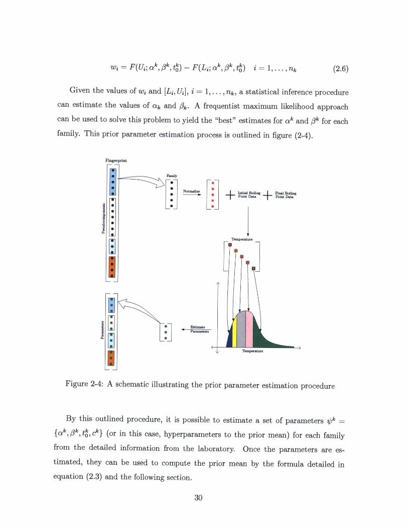
wi = F(Ui;ak I k,tk) - F(Li;ak Ik,tk) i = 1,...,n (2.6)

Given the values of wi and [Li, U], i = 1,... ,nk, a statistical inference procedure

can estimate the values of ak and #k. A frequentist maximum likelihood approach

can be used to solve this problem to yield the "best" estimates for ak and #k for each

family. This prior parameter estimation process is outlined in figure (2-4).

Fingerprint

IS

.1I0.

I0.

Figure 2-4:

Family

Normalize

Estimate

Point Data Point Data

I

A schematic illustrating the prior parameter estimation procedure

By this outlined procedure, it is possible to estimate a set of parameters 0'/ -

{a k, tk, t ck} (or in this case, hyperparameters to the prior mean) for each family

from the detailed information from the laboratory. Once the parameters are es-

timated, they can be used to compute the prior mean by the formula detailed in

equation (2.3) and the following section.

30

Prior covariance

Ideally, the prior covariance is a matrix whose (i, j)-th entry captures the how the

concentrations of pseudo-compound i and j vary together. However, as a result of the

large underconstrained nature of the feed reconstruction problem, it is often better

to use some simplifying assumption to reduce the number of unknown covariance

parameters. In this case, the prior covariance matrix E is assumed to be of the form

a21m, where o > 0 is a variance parameter and Im is the m x m identity matrix. Now,

the only parameter that has to be tuned is o-.

The variance parameter indicates the degree-of-belief in the similarity of the feed

that is analyzed in the laboratory and the feed that is being analyzed in the refinery.

If the 2 types of feed are believed to be similar (sourced from the same reservoir or

neighboring reservoirs, for example), then a lower value of the variance parameter can

be used. If the two feeds are very different, then a higher value of variance would be

appropriate.

2.2.3 Likelihood

If V denotes the vector of bulk measurements that are collected in the plant, then

the likelihood function L(DIY) is a function that quantifies how likely the observed

plant data are, given realization of Y.

To construct this likelihood function, a measurement model is required. A mea-

surement model is a function that calculates the bulk properties for a given realization

of Y. If the vector of calculated bulk properties is denoted by Dck, the measure-

ment model is a function f, such that Dac f(Y). For the sake of convenience,

the Bayesian feed reconstruction model assumes that this function f is linear in Y.

While this idea ensures that the expression for the posterior distribution can be de-

rived analytically, this is not a necessary condition.

While the linearity assumption might seem unjustified, the choice of the structure

of Y makes it convenient to reconstruct several types of bulk measurements typically

encountered in a refinery in a linear fashion. In the pseudo-compound and tempera-

31

ture matrix (which was described in the previous subsection), the columns correspond

to the distillation temperature ranges. So, the weight fraction of the feed that is dis-

tilled in each temperature range can be recovered as a simple column sum, which is

a linear operation on Y. Bulk concentrations of atomic species, such as sulphur, can

be calculated as

Scalc =i ) Yi (2.7)

where MWs is the molecular weight of sulphur, MWy, is the molecular weight of

the pseudo-compound corresponding to Y. This is also a linear function of Y.

Since the calculated bulk properties can never match the actual observed bulk

properties (D,), an error model on the observation is also required. For simplicity's

sake, a Gaussian measurement error is associated with each measurement. If the

vector of observed bulk properties is denoted as DV,, then

(Dos) = (Dea1 c) + Ei, ei . A(O, of), i = 1, ... , nbulk (2.8)

where nekd is the number of bulk measurements. Here, ei is a Gaussian measure-

ment noise in the i-th bulk measurement with zero mean and variance o (which is

usually available as instrument error). It is assumed that all the measurement errors

are independent of each other.

With these assumptions, the likelihood function can be written as

£(DIY) = exp (D' f (y)) T E 1 (DP - (y)) (2.9)2

Em is a diagonal matrix where the (i, i)-th entry corresponds to the measurement

error in the i-th bulk measurement.

2.2.4 Posterior distribution

With the prior distribution and the likelihood, the posterior distribution can now be

computed using equation (1.1) as

32

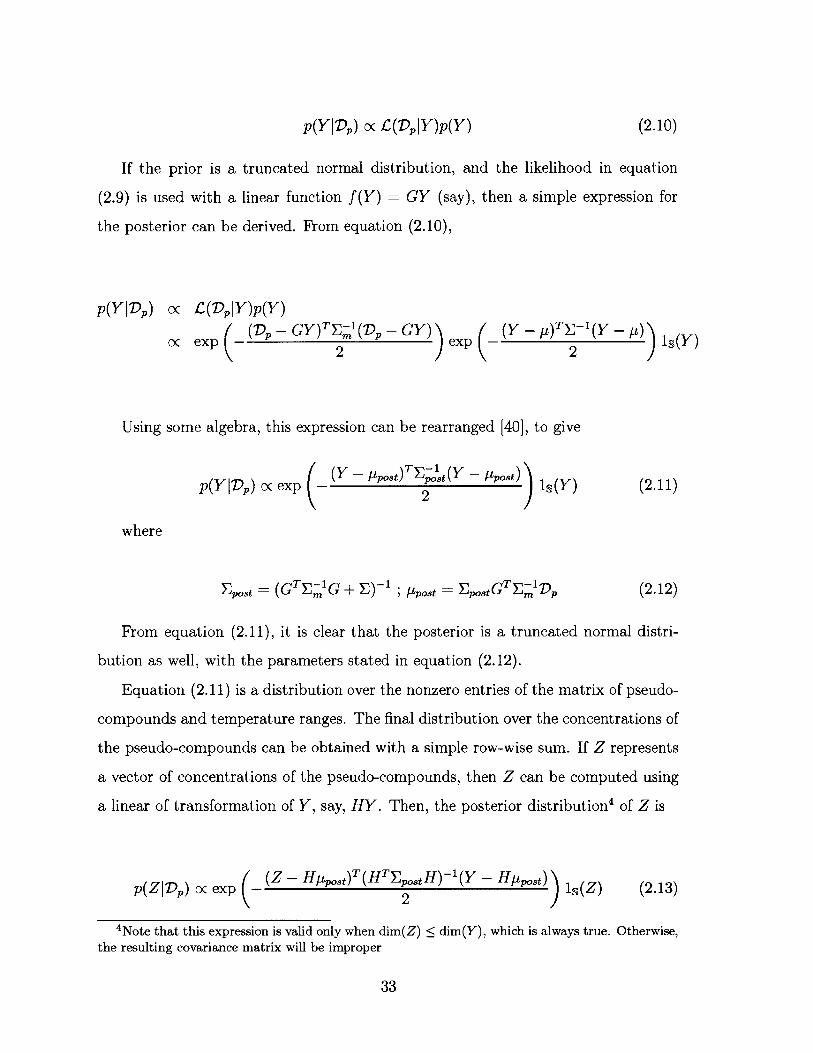
p(Y|D,) oc L(D,|Y)p(Y) (2.10)

If the prior is a truncated normal distribution, and the likelihood in equation

(2.9) is used with a linear function f(Y) = GY (say), then a simple expression for

the posterior can be derived. From equation (2.10),

p(YID,) c L(D|Y)p(Y )

C exp (Dp - GY)TE -1(DP - GY) (Y)(Y - p)TE-1(Yoc xp2 2 1s(Y

Using some algebra, this expression can be rearranged [40], to give

(Y - p TE) i t (Y - pt.0p(YID,) oc exp (Y - 2 1s(Y) (2.11)

where

E. =(TF 1i G + E )- ; ypat = Epst G T E -1% 3Zpost =(GT3l ±M Z) tM ~tT~ (2.12)

From equation (2.11), it is clear that the posterior is a truncated normal distri-

bution as well, with the parameters stated in equation (2.12).

Equation (2.11) is a distribution over the nonzero entries of the matrix of pseudo-

compounds and temperature ranges. The final distribution over the concentrations of

the pseudo-compounds can be obtained with a simple row-wise sum. If Z represents

a vector of concentrations of the pseudo-compounds, then Z can be computed using

a linear of transformation of Y, say, HY. Then, the posterior distribution4 of Z is

p(ZID,) oc exp (Z - H1sost)T(HTEpostH)1(Y - Hip8 t)) 1,(Z) (2.13)

4Note that this expression is valid only when dim(Z) ; dim(Y), which is always true. Otherwise,the resulting covariance matrix will be improper

33

2.3 Advantages of the Bayesian approach

The Bayesian feed reconstruction procedure constructs a posterior distribution over

the concentrations of each pseudo-compound by combining the laboratory informa-

tion and plant data in a systematic manner. Unlike previous composition model-

ing techniques, the explicit identification of the prior distribution and the likelihood

makes it easy to add new sources of information while retaining intuitive knobs on

the reliability of the new data, compared to existing information.

If a new kind of laboratory measurement is made, for instance, it can be incor-

porated into the reconstruction process by suitably modifying the prior distribution.

On the other hand, if a new bulk measurement is made, it can be appended to the

existing measurement vector D,, as long as it has an appropriate measurement model

(preferably, linear) and an associated measurement error (of).

The notion of uncertainty is directly built into the Bayesian inference procedure.

The concentrations Z are assumed to be realizations of a random variable with a

multivariate probability distribution. Techniques to perform sensitivity analysis and

experimental design on the reconstruction or any subsequent downstream process are

readily available.

2.4 Exploring the posterior distribution

Inference procedures on random variables usually focus on expectations or integrals

of the probability distribution function. For example, one quantity of interest to

the modeler might be the average concentration, expressed as E(Z). To analyze the

variation of the concentration of a pseudo-compound, the modeler might choose to

analyze the percentiles of the probability distribution function (which is an integral

of the density function).

The posterior probability distribution p(ZID,) is a high-dimensional distribution

(since reconstruction procedures employ a high number of pseudo-compounds to im-

prove modeling accuracy). While the expression for this distribution is simple, there

34

are no closed-form expressions to estimate the moments or expectations of this dis-

tribution p(Z|D,).

To understand and utilize the resulting posterior distribution, there is a clear need

to evaluate arbitrary expectations of Z. In the next section, we shall motivate the

idea on how to evaluate these high-dimensional integrals.

35

Chapter 3

Computational aspects of feed

reconstruction

3.1 Introduction

In the previous section, a Bayesian formulation for the feed reconstruction problem

was proposed and an expression for the posterior density function was derived. To

analyze the posterior distribution, it often becomes necessary to evaluate integrals of

the form

Ez[f(zi, .. . ,z.)] = ---. I f(zi, ... ,z.)p(zi, .. ., z.)dS(zi,. . ., z.) (3.1)ScRn

Where Z is a random variable with a multivariate probability density function

p(zi,... , z,) that is truncated on a set S. In the feed reconstruction case, the proba-

bility density function would be the Gaussian density function with some mean and

covariance parameters, and S would be the set

n

S= {z c R" n zi = 1, zi > 0, i = 1...n} (3.2)

This set corresponds to a scaled version of the standard (n - 1)-simplex, which is

37

/ 0

0204

0.2J

Figure 3-1: The standard 2-simplex corresponding to the set S =

{z E R3 | 1 =3 1, zi >O, i={1,2,3}}

sketched in figure (3-1).

In general, there are no analytical techniques to evaluate these integrals for cases

where the density p(z) is the multivariate truncated normal distribution. These distri-

butions play an important role in a wide range of modeling applications even outside

feed reconstruction [3, 28], so devising a good algorithm to evaluate these integrals

is important. Numerical integration (or, quadrature) techniques are algorithms that

are used to compute approximations definite integrals. If the integrals are univariate,

there are several quadrature techniques that are readily available[32]. If the integrals

are multivariate, numerical integration (or, cubature) using repeated application of

1D quadrature techniques does not scale well with the number of dimensions. For

high-dimensional numerical integration problems, Monte Carlo methods or sparse

grid techniques are usually the methods of choice.

3.1.1 Monte Carlo methods

Monte Carlo (MC) methods are computationally intensive stochastic sampling tech-

niques that can be used to numerically evaluate integrals. They rely on repeatedly

sampling from random variables to carry out numerical computations. The idea was

first proposed and developed by mathematicians and physicists at the Los Alamos

labs during World War II. With the exponential increase in computing power, Monte

38

Carlo methods 1 are now very popular and widely used in different areas of compu-

tational science.

One of the biggest advantages of MC methods lies in the scaling of the error in

the numerical estimate Iet. If equation (3.1) is evaluated by repeatedly applying ID

quadrature techniques, the error bound |Iet - Il is O(N-r/d), where d is the number

of dimensions, and r is typically 2 or 4. As a result, typical quadrature methods

become too computationally expensive outside low-dimensional (d < 7) problems.

However, the error bound in MC methods is O(N-1/ 2 ), independent of the number

of dimensions. This makes MC methods particularly attractive for high dimensional

problems[1].

3.2 Numerical integration using Monte Carlo sam-

pling

The Monte Carlo integration algorithm numerically computes equation (3.1) by gen-

erating N random points zi, i = 1, ... , N, such that z~ p(z)), where p(z) is assumed

to be supported on S. Then, the value of the integral can be approximately computed

as the arithmetic mean of the function evaluations at zi [24]. Mathematically,

Ez [f (zi, . . . , z.) ] ~zz IMC E~ - --. , z'), i =l1,2, -. -IN (3.3)i=1

Note that this method can also be used to numerically integrate any function, if

the probability density is chosen to be the uniform density function (assuming that

S is compact) 2.

In the feed reconstruction problem, the probability distribution of interest p(Z) is

'It is worth mentioning that MC methods nowadays refer to a very broad class of algorithms. Weare particularly interested in MC methods for numerical integration, so any mention of MC methodsare in the context of numerical integration

2 While it might be tempting to evaluate Ez[f(zi,..., zn)] by numerically integrating g(Z)f(Z).p(Z) using a uniform distribution, it should be noted that doing so would drastically reducethe accuracy of the Monte Carlo method[24]

39

3a multivariate Gaussian distribution that is truncated on a simplex

Monte Carlo integration relies on the ability to generate (almost) independent

samples from our truncated normal distribution p(z), to ensure the accuracy of the

Monte Carlo estimate[43]. While several sampling techniques exist in literature[24],

the next section focuses on a particular class of methods called Markov Chain Monte

Carlo methods.

3.3 Markov chain Monte Carlo

Markov chain Monte Carlo (MCMC) methods are a class of algorithms that sample

a probability distribution, p(z), by generating a Markov chain that has the same

stationary distribution [18]. With the rise of computer processing power, there has

been an explosion in the research and development of MCMC algorithms [8].

3.3.1 Literature Review

Geweke [17] first addressed the problem of sampling from a normal distribution sub-

ject to linear constraints using an MCMC algorithm. However, the method was lim-

ited and allowed only for a fixed number of inequality constraints. Rodriguez-Yam et

al. [38] extended Geweke's method to remove the restriction on the number of con-

straints, and introduced additional scaling in the problem to improve the sampling.

Dobigeon et al. [13] explicitly address the problem of sampling from a multivariate

Gaussian that is truncated on a simplex, by combining a Gibbs algorithm along with

an accept-reject framework to sample from the 1-dimensional truncated Gaussian

distribution [37].

Apart from the Gibbs family of algorithms, Smith et al. [6] proposed a particu-

lar type of random walk samplers called Hit-and-Run samplers that can be used to

sample from distributions restricted to convex domains. Recently, Pakman et al. [30]

3 For the sake of simplicity, this section will only discuss sampling from truncated normal distri-butions. Sampling from arbitrary posterior distributions truncated on simplex-type constraints isan even harder problem.

40

proposed a Hamiltonian Monte Carlo algorithm to sample from truncated Gaussian

distributions.

3.3.2 Sampling problem

To analyze the results of the Bayesian model, we require samples from of the posterior

distributions, which are multivariate normal distributions truncated on the standard

simplex. However, for the sake of completeness, we shall analyze samplers that can

generate samples from normal distributions that are truncated on convex polytopes4 .

Before we explore the different types of algorithms that can be used to sample from

normal distributions truncated on convex polytopes, we can simplify the given sam-

pling problem.

Consider sampling from the multivariate Gaussian distribution p(z) = N(p, E),

such that the samples z obey

Amxnz = bmxi (34)

Ckxnz < d y1

where m and k are the number of equality and inequality constraints respectively.

These feasibility constraints correspond to a convex polytope in R".

Note that the case of the truncated The Gaussian distribution can be conditioned

such that the resulting function is a distribution only in the subspace defined by the

equality constraints. This can be achieved by considering a new random variable

W = AZ, and deriving a joint distribution for the random variable pair V = (Z, W).

Once the joint is obtained, setting W = b, will result in a conditional distribution

p(ZIW = b).

Mathematically, the random variable W is Gaussian (since affine transformations

of Gaussian random variables are Gaussian). This means that the joint distribution

of Z and W is also Gaussian, with mean

'Simplices are special cases of convex polytopes

41

i= [[ p(Ap)T|T (3.5)

and covariance

(3.6)

Then, the conditional distribution p(ZjW = b) = N(pc, Ec) [39], where

Ac = p' + E ETAT( AAT )-(b - Apt) (3.7)

and

EC = E- T AT(AEAT) -AE (3.8)

Now, any sample Z ~ (jp, Ec)", will obey the equality constraints in equation

(3.4).

Sampling from the n - m dimensional space spanned by the eigenvectors corre-

sponding to nonzero eigenvalues ensures that the resulting samples always obey the

equality constraints. If we represent the eigenvalue decomposition of Ec as

Ec = QAQT (3.9)

If the zero eigenvalues and corresponding eigenvectors are deleted, then the trun-

cated eigenvalue decomposition may be denoted as

EC = UAUT (3.10)

This means that the problem can now be reparametrized in terms of an indepen-

dent multivariate normal random variable W ~ N(O, I), where I denotes an identity

5Ec is a rank-deficient covariance matrix, with rank = n - in-, where fii is the number of inde-pendent equality constraints ( ; m) in equation (3.4)

42

rTAT

AEATLAE

matrix, using the linear relation

Z= MW +pc (3.11)

where

M = QA1/2 (3.12)

Note that W is an (n - m)-dimensional random vector. The inequality constraints

can be rewritten by substituting the expression in (3.11) in equation (3.4) as

Mw + Cyc < d (3.13)

where w denotes a sample of W. Now, the original problem reduces to one of

sampling from a truncated (n - m)-dimensional independent multivariate Gaussian

random variable, truncated to a convex polytope defined by equation (3.13).

In the following sections, 3 types of samplers Markov chain Monte Carlo samplers

will be discussed.

3.3.3 Gibbs sampler

The Gibbs sampler [18] was introduced in MCMC literature by Gelfand and Smith [16]

as a special case of the Metropolis-Hastings algorithm. The Gibbs algorithm for

sampling from an arbitrary distribution p(w) truncated to a set S C R' is presented

below:

Gibbs sampler

Step 1: Choose a starting point wo E S, and set i = 0

Step 2: Update each component of wz by sampling from the full conditional

distributions along each coordinate, (i.e.)

w+ 1 +1.0 1, +,..., w), for j = 1... n

43

Step 3: Set i= i + 1, and go to Step 2

In general, it is hard to obtain conditional distributions truncated to the feasi-

ble set S. However, when the set S corresponds to a simplex (or more generally, a

polytope), closed form expressions for the conditional distributions are easily avail-

able [37].

A Gibbs type sampler can be implemented for this problem, since the conditional

distribution for each component is the standard normal distribution K(O, 1) truncated

to a range. The lower and upper limits of this range can be computed using equation

(3.13).

Suppose that at iteration k, we wish to generate a sample of the i-th component

wk, say wk. The upper and lower limits of the conditional distribution range is given

by the minimum and the maximum of the vector wk , which is calculated as

S= d - Cyc - Mjii2j (3.14)

where M,i denotes the matrix M with the i-th column removed, and Gej is the

vector [wk . _1 , k, -- ] The modified Gibbs algorithm can be summa-

rized as below:

Modified Gibbs sampler

Step 1: Choose a starting point w0 that satisfies equation (3.13), and set i = 0

Step 2: Update each component of W' by sampling from a truncated normal

distribution along each coordinate, (i.e.)

w+1 ~ Nr(0, 1) , wj+1 G [a+1, b+1

where a + and bj+1 are the minimum and maximum of w' 1 , given by

equation (3.14)

Step 3: Set i= i + 1, and go to Step 2

44

To complete this procedure, we need to sample from a series of 1-dimensional

truncated normal random variables. There are several algorithms [11, 37] available in

literature to solve this problem, and any one can be suitably applied to sample from

the conditional distribution at each step.

3.3.4 Hit-and-run sampler

d

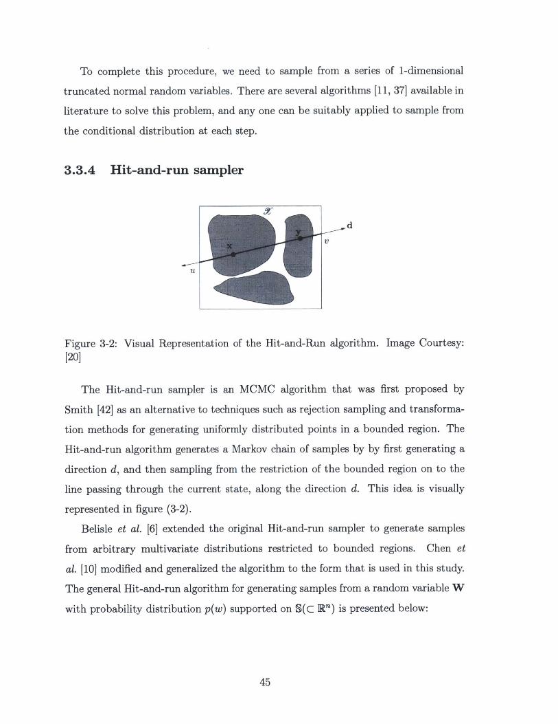
Figure 3-2: Visual Representation of the Hit-and-Run algorithm. Image Courtesy:[20]

The Hit-and-run sampler is an MCMC algorithm that was first proposed by

Smith [42] as an alternative to techniques such as rejection sampling and transforma-

tion methods for generating uniformly distributed points in a bounded region. The

Hit-and-run algorithm generates a Markov chain of samples by by first generating a

direction d, and then sampling from the restriction of the bounded region on to the

line passing through the current state, along the direction d. This idea is visually

represented in figure (3-2).

Belisle et al. [6] extended the original Hit-and-run sampler to generate samples

from arbitrary multivariate distributions restricted to bounded regions. Chen et

al. [10] modified and generalized the algorithm to the form that is used in this study.

The general Hit-and-run algorithm for generating samples from a random variable W

with probability distribution p(w) supported on S(c R") is presented below:

45

Hit-and-run sampler


Step 2: Generate a direction d1 on the boundary of the unit sphere in R" from

a distribution v

Step 3: Find the set Si(d, w)= {A E Rlwt + Ad E S}

Step 4: Generate a signed distance A" ~ g(Ald, w'), where A E

Step 5: Generate ui ~ Unif [0, 1]

Step 6: Set y wi + Ad, and set wi+1 _y, if .u < min {1, ai(wi, y)}

w, 6 otherwise

Step 7: Set i i + 1, and go to Step 2

where a' denotes an acceptance probability. Note that this sampler works even if

the function p(w) is only known up to a multiple of a density function'. To complete

the algorithm, we have to specify the direction distribution V from Step 2, the density

g in Step 4, and the acceptance probability a' in Step 6. Belisle et al. [6] prove that

if v is chosen to be the uniform distribution on the n-dimensional unit hypersphere 7,

and g(Ald, w) is the restriction of p(w) on the set S', then a' always equal to 1.

In general, restrictions of arbitrary probability distribution on line sets (such as S')

are not easy to compute.However, closed form expressions exist for the multivariate

uniform and normal distributions.

In particular, we are interested in sampling from the restriction of a truncated

normal distribution on to a line along d. The expression for the restriction of a

truncated normal density on a line passing through a point x along a direction d is

derived in appendix B.6 This means that fs P(w1... -n)dwi ... dwn # 17 We can generate uniform directions on the surface of the n-dimensional hypersphere by first

generating a sample from an n-dimensional multivariate i.i.d Gaussian, and setting the directiond* to the normalized sample. Mathematically, i ~ K(Onx 1, UInxn); di = i/III => di is uniformlydistributed on the unit sphere (0 and II denote a vector of zeros and an identity matrix respectively)

46

As a final note on hit-and-run sampling algorithms, it is worth observing that if

the direction distribution v is restricted to be an equally weighted discrete probability

distribution along n directions, where the n directions are the coordinate directions,

and the density of A', is the restriction of the density p on the set S', then this

algorithm becomes the random scan Gibbs sampling algorithm [21].

As in the Gibbs sampling case, consider the problem of sampling from the standard

multivariate normal distribution in (n - m) dimensions truncated to the polytope de-

fined by equation (3.13). If we denote the feasible set as S, the hit-and-run algorithm

to sample from this density is summarized below:

Modified hit-and-run sampler


Step 2: Generate a direction d by first generating z' - K(0, I), then setting

di = zz/||zI||

Step 3: Find the set S (di, xz) [a', bi], where as and b' are the largest and

smallest values of A, such that w' + Ad satisfies equation (3.13)

Step 4: Generate a signed distance A' from the truncated normal distribution

N ( (&i)2), A' c [a', b'], where t? and 05 are given by 8

(di)Tdi

a (di)Tdi 1

Step 5: Generate ut ~ Unif [0, 1]

i+1 y, if u < min{11, a'(ylw')}Step 6: Set y = w' + Azd, and set wi+1 -

tw , otherwise

Step 7: Set i = i + 1, and go to Step 2

8 For a proof, the reader is referred to appendix B

47


The Gibbs sampling and Hit-and-run algorithms fall under the class of random walk

samplers, where the next sample depends on the value of the current sample. While

these type of samplers are convenient, they often result in samples that are increas-

ingly correlated as the dimensionality of the underlying distribution rises [30].

Independence samplers are a class of Metropolis-Hastings algorithms, where the

sample that is proposed does not depend on the value of the previous sample. These

types of samplers are advantageous, since a well designed independence sampler

should scale better than the Gibbs or Hit-and-run algorithm with an increase in

the dimension of the distribution. The convex nature of the simplex constraint com-

bined with the unimodality of the normal distribution make the problem particularly

amenable to the design of an independence sampler. In this section, we shall con-

struct an independence sampler, which is a modification of the Directional metropolis

algorithm proposed by Eidsvik et al. [14].

As before, consider the problem of sampling from a random variable W distributed

with an (n - m)-dimensional multivariate standard normal density truncated to the

polytope defined by

dMw +Cpe ; d

where w is a sample of W. To generate samples from this distribution, consider

an independence sampler of the form

W = Wma + au , a > 0 (3.15)

where wma, refers to the maximum a posteriori probability (MAP) estimate of the

truncated normal distribution corresponding to W '. The p thus generated is a point

on the line passing through wmap, along a direction u at a euclidean distance of a from

Wmap (Note that (Note that ||uI| = 1). By sampling from appropriate distributions,

it is possible to generate every point in the polytope defined by equation (3.13) with

9This MAP estimate can be computed using a simple constrained optimization routine

48

a unique combination of u and a. A general independence sampler [24] is outlined

below:

Metropolized independence sampler

Step 1: Choose a starting value w0 that satisfies equation (3.13), and set i 0

Step 2: Draw w i+1 - q(i+1)

Step 3: Draw cZ ~ Unif [0, 1]

Step 4: Set

+1 i+ ,if c2 < min{1, r(wi, Wi+1)}

wi , otherwise

Step 4: Set i i + 1, and go to Step 2

Here, q(w) is called a proposal density, r(-,.) denotes the acceptance ratio at

iteration t, and Unif [0, 1] represents the uniform distribution over [0, 1]. Let us

denote the underlying standard truncated normal distribution of the random variable

W as ir(w).

The Metropolis algorithm is completely specified once the proposal density and

the acceptance ratio are fixed. The acceptance ratio is a quantity that ensures that

the samples that are generated from the Metropolis algorithm represent samples from

the ir(w), and is fixed by the detailed balance condition. The proposal density, on the

other hand, is a distribution whose choice determines the quality of the samples that

are generated. In general, the closer the proposal density q(w) to the actual density

ir(w), the better the quality of samples generated. First, we shall decide on the

proposal mechanism for the independence sampler. Once the proposal distribution is

fixed, the acceptance ratio can be derived by enforcing the detailed balance condition.

Any sample w is generated by first choosing a particular direction u, and then a

distance a, such that the w calculated from equation (3.15) remains in the polytope

defined by equation (3.13). As a modeling choice, we model the direction using a

49

projected normal distribution, and the distance a using a Gaussian random variable.

The 2 proposal distributions are discussed in the following subsections.

Directional proposal distribution

The direction u is generated from an (n - m)-variate projected normal distribu-

tion [25] which is parametrized by a mean vector (pd) and a covariance matrix (Ed).

The sample u from the projected normal distribution is generated by first sampling

x ~ f (Ald, Ed), then setting u = x/||xI|. In this case, the sample u lies on the

(n - m) dimensional unit sphere. For more information about the projected normal

distribution and directional statistics, the reader is referred to appendix C.

Pukkila et al [33] derived an analytical expression for the density function of

the projected normal distribution with respect to the surface element dWn-.m on the

(n - m)-dimensional unit sphere, as

p(ulpd, Ed) = |22rEdi1/2 Qmn)/2 In-m(Q2Q31/2) [-2-(Q1 - Q2Q3)] (3.16)

where Q1 = jE-Ipa, Q2 = pE-lu and Q3 = UTE-lu.

In-m(-) is an integral that can be evaluated using a recursive relation, which is

listed in appendix C. This distribution reduces to the uniform distribution on the

unit sphere if pd is chosen to be zero and Ed is chosen to be the identity matrix.

For the sake of convenience, the covariance matrix Ed is chosen to be an identity

matrix. The vector pd acts as a concentration parameter (refer appendix C) that

controls the clustering of the samples from the projected normal distribution. This

provides a useful tuning parameter for the direction proposal, since it is reasonable

to expect the directions of samples to cluster based on the location of the MAP point

within the feasible region. For example, if the MAP point were to lie at the barycenter

at the polytope, the directions to that originate from the MAP can be expected to

be more or less uniform. On the other hand, if the MAP point were to lie close to an

edge or a vertex, most of the samples would have directions towards the interior of

the polytope.

50

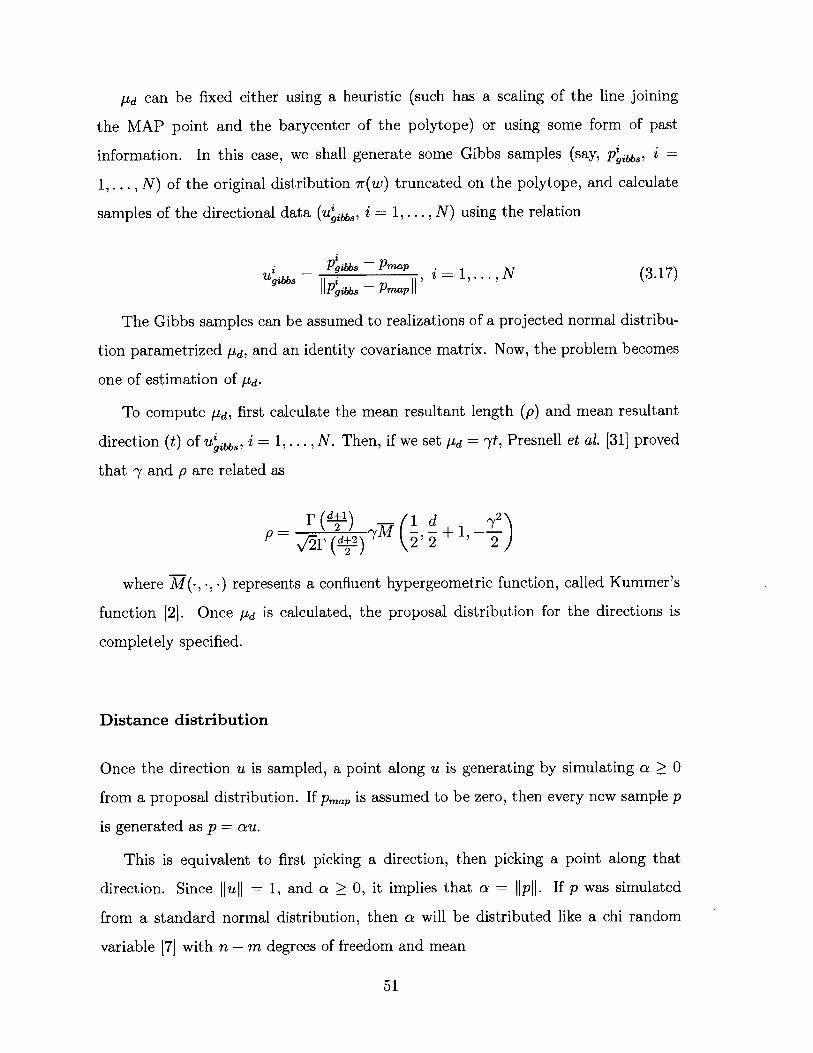
pUd can be fixed either using a heuristic (such has a scaling of the line joining

the MAP point and the barycenter of the polytope) or using some form of past

information. In this case, we shall generate some Gibbs samples (say, p i =

1,..., N) of the original distribution ir(w) truncated on the polytope, and calculate

samples of the directional data (U i = 1,..., N) using the relation

Pgibbs -Pa

I mrap , = 1, ... , N (3.17)

The Gibbs samples can be assumed to realizations of a projected normal distribu-

tion parametrized pd, and an identity covariance matrix. Now, the problem becomes

one of estimation of Ad.

To compute pd, first calculate the mean resultant length (p) and mean resultant

direction (t) of u'ib,, i = 1,..., N. Then, if we set pd = -t, Presnell et al. [31] proved

that 7 and p are related as

IF (-±21 ( d 72)

V/2Tr (!!L2) 2

where M(-,-,-) represents a confluent hypergeometric function, called Kummer's

function [2]. Once yd is calculated, the proposal distribution for the directions is

completely specified.

Distance distribution

Once the direction u is sampled, a point along u is generating by simulating a > 0

from a proposal distribution. If pmap is assumed to be zero, then every new sample p

is generated as p = au.

This is equivalent to first picking a direction, then picking a point along that

direction. Since ||ull = 1, and a > 0, it implies that a = ||pil. If p was simulated

from a standard normal distribution, then a will be distributed like a chi random

variable [7] with n - m degrees of freedom and mean

51

v/-1((n - m + 1)/2)F((n - m)/2)

where IF(-) denotes the Gamma function. In other words, this means that most

of the samples from a high-dimensional Gaussian distribution will lie on a shell of

radius [pa ~ /n -/ m. This phenomenon is sometimes referred to in literature as

concentration of the Gaussian measure [15]10.

This means that a good proposal for a is a Gaussian that is centered at pa, with

unit variance. Note that the variance of the chi distribution (ao n - m - [L2 ) can

be used as a good guess for the variance of the Gaussian proposal. However, for the

sake of convenience, we shall use the unit variance proposal. While the lower bound

for a is zero, the upper bound b is the largest positive real number that satisfies

b( Mu) < d - Mp,,,, - Cpe

This implies that the proposal distribution for alpha is a normal distribution

.A(pa, 1), truncated to the closed interval [0, b]. The probability density function at

any point a E [0, b] for the distance proposal is

q(alu) - (a ) (3.18)b(b - pc,) - b(pa)(

where 0(-) and <D(.) represent the probability density and cumulative density func-

tions of the standard normal density respectively.

Now that the proposal distributions have been fully specified, the acceptance

ratio can be derived by writing the detailed balance condition. To avoid cumbersome

notation, let x denote the current sample (w'), and y denote the sample at the next

iteration (w i+1). For the Metropolis algorithm to work, the stationary distribution

of the Markov chain that is generated should be the density that is being sampled 1 .

10 For a good introduction to the phenomenon of measure concentration, the reader is referredto [5]

"Another important property, called reversibility, can be easily verified to hold for the proposedalgorithm [36]

52

The stationarity condition can be expressed as

Jr(y) = Ir(x)A(x, y)dx (3.19)

Here, A(x, y) denotes the actual transition function from x to y, which is not

necessarily the proposal distribution [24]. In fact, for the Metropolis algorithm, the

actual transition function can be written as

A(x, y) - q(y)min {1, r(x, y)}

where q(-) is the independent proposal density and r(-, -) is the acceptance ratio.

Since the samples themselves are described in terms of u's and a's, equation (3.19)

can be re-written as

7r(ay, uy) = Jr(ax, ux)A([ax, u2], [acy, u])a-'daxdwx (3.20)

where dw is an infinitesimal surface element on the n - m dimensional unit sphere,

and

X =Pmap + a2U,

and y = Pmap + ayu,

where the directions dx and d is simulated from a projected normal distribution

parametrized by ptd. The distance ax is a sample from a normal distribution with

mean [Lx and unit variance, truncated on the interval [0, bx], while ao is a sample

from a normal distribution with mean py and unit variance, truncated on the interval

[0, by].

The detailed balance [24] condition automatically ensures that equation (3.20) is

always satisfied. The detailed balance in this case can be written as

-7r(aey, uy)A([aey, u,], [ax, ux])a,"-" = 7r(ax, ux)A([ax, ux], [aey, Uy])an"-" (3.21)

53

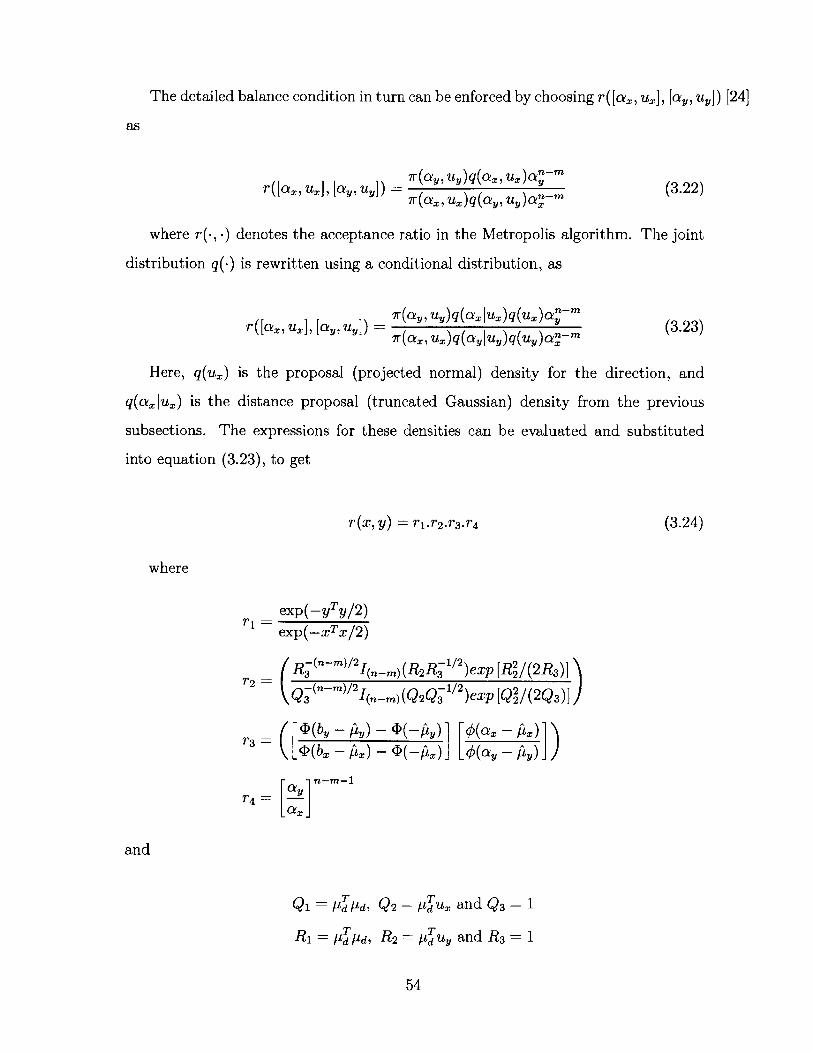
The detailed balance condition in turn can be enforced by choosing r([ax, u.], [a,, uy]) [24]

as

7r (ay, uy) q(ax, ux) a "-mr([a., u-], [ay,u]) - 7r(aI q(y _ (3.22)

r(a, ux)q(ay, U)a-n(3.22)

where r(., -) denotes the acceptance ratio in the Metropolis algorithm. The joint

distribution q(-) is rewritten using a conditional distribution, as

7r (ay, uy) q(ax|ux) q(ux) a,"-"r([ax, u2], [ay, uy]) = (3.23)

7r(ax, ux)(q2(ay3uy)q(y)an-m

Here, q(ux) is the proposal (projected normal) density for the direction, and

q(ax|ux) is the distance proposal (truncated Gaussian) density from the previous

subsections. The expressions for these densities can be evaluated and substituted

into equation (3.23), to get

r(x, y) = r1.r 2 .r3 .r 4 (3.24)

where

exp(-yTy/2)exp(-xTX/2)

R2 (3-)/I(n-m)(R2R31/)exp [R22/(2R3)]

Q3(n-m)/ 2 n (Q2Q31/2 )exp [Q /(2Q3)]

<D~~~~by) - AO b(A)~(ax - AX)~<brb - AX) -<(AX) _#(a, - AY)_f

-n-m-1r 4 = -aI[ax

and

Q1 = Pdpa, Q2 - ptd and Q3 1

R1 = pt pa, R 2 = /4Tu and R 3 1

54

With this proposal distribution and acceptance ratio the modified Metropolized

independence sampler is presented below:

Directional independence sampler

Step 1: Calculate the MAP point of the truncated normal distribution, Wmap,

using an optimization routine

Step 2: Choose a starting value w0 that satisfies equation (3.13), by simulating

a value a0 and do from the proposal densities and set i = 0

Step 3: Draw di+1 q(di+1), and '+ qg( i+ i+1),

W i+1 = Wmap + a i+1di+1

Step 4: Draw cZ ~ Unif [0, 1]

Step 5: Set

wi++1Wi+ W+ if c' < min{ 1, r(w', ' i+1)}

w' , otherwise

where r(., -) is the acceptance ratio defined in equation (3.24).

Step 6: Set i= i+1 , go to Step 3

3.4 Summary

In this section, we have outlined some of the computational issues that can arise

when analyzing the posterior distribution of the Bayesian feed reconstruction model.

To overcome these challenges, we decided to adopt a Monte Carlo approach. Since

the Monte Carlo approach requires an efficient generation of samples from the pos-

terior distribution, we reviewed 3 sampling algorithms. In the next chapter, we shall

implement the samplers and compare their relative performance in a set of test cases.

55

Chapter 4

Results

In the following sections, we shall compare the performance of the different samplers

that were discussed in the previous chapter. First, we shall implement a few low

dimensional test cases, to test the accuracy of the various samplers. Once we study

the performance of these algorithms in the lower dimensional test cases, we shall apply

them to sample a posterior (high dimensional) distribution from a feed reconstruction

example on a real life data set.

4.1 Low dimensional examples

We construct three different three dimensional Gaussian distributions that are trun-

cated on the standard 2-simplex (say, S), where S ={x e R 3 |1 + X2 + X3 - 1, X; >

0, i = 1, 2, 3}. In the three cases, we shall vary the mean (p) and covariance matrix

(E) parameters associated with each Gaussian distribution.

0 1 0 0

Case l: p= 0 ,E= 0 1 0

0 0 0 1

0 0.1 0 0

Case2: I 1 ,E= 0 0.1 0

0 0 0 0.1

57

0 25 -25 -50

Case3: t= 0 -25 25 -50

1 -50 -50 100

In all these three cases, the normal distribution is truncated to the set S . To visu-

ally verify the working , we run the algorithm on each of the test cases, and produce

a scatter plot of the samples generated on the simplex, along with the trace of the

samples in each coordinate, and the autocorrelation of the samples generated along

each dimension. The scatter plot and the sample trace allow us to visually inspect

if the algorithm generates chains that mixing well [8]. Autocorrelation along each

sample dimension numerically tells us how well the chain is mixing. Low autocorre-

lation implies that the samples that are being generated are nearly independent, so

any Monte Carlo estimate would require a relatively low number of samples to reach

a desired accuracy. On the other hand, large autocorrelation in the samples implies

that one would require a significantly larger number of samples to reach the same

accuracy [43].

To numerically verify the samplers, we compute the mean of the truncated normal

distribution using a 2-D quadrature routine (such as integral2 in MATLAB) on

the simplex, and then compare it with the mean of 10' samples generated by the

algorithm. By visually inspecting the samples and comparing the first moment of

the truncated distribution along with the sample mean, we can decide if the sampler

functions efficiently and accurately.

58

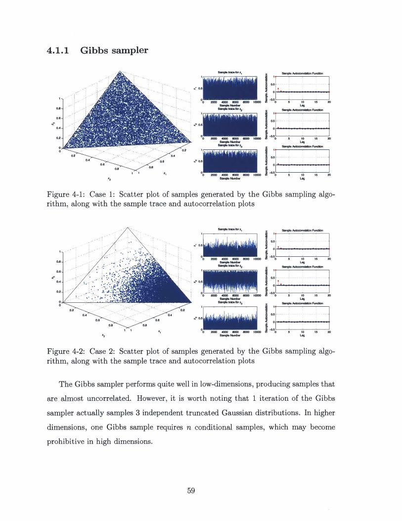
4.1.1 Gibbs sampler

Sample Auto8oreiallon Funtion

10000 0 5 10 Is 20Log

Sam,ple Aub00meicm Function

0

10000 0 a 10 15 20Log

SOROS Aulocr1eltsion Funcion

0

1000 0 2 1 0 15 20Log

Figure 4-1: Caserithm, along with

1: Scatter plot of samples generated by the Gibbs sampling algo-the sample trace and autocorrelation plots

Samiple ta for Z'

.0.5

0 2000 4000 200 8000 100Samos ""ber

Samoa We br z

' 0.a

0 11 1 ' 1 11 1' 1I 1 ~ 1o 20o 00080 so 10000

SO Np ler

I~~~~~~ I

X1

Sample Autciaffllron Fundion

-00 10 15 20

Sample AdoriaimFunction

0 005 20Lag

Sample Patocorrelalon Fundion

as - - -00 5 10 is 20

Log

Figure 4-2: Case 2: Scatter plot of samples generated by the Gibbs sampling algo-rithm, along with the sample trace and autocorrelation plots

The Gibbs sampler performs quite well in low-dimensions, producing samples that

are almost uncorrelated. However, it is worth noting that 1 iteration of the Gibbs

sampler actually samples 3 independent truncated Gaussian distributions. In higher

dimensions, one Gibbs sample requires n conditional samples, which may become

prohibitive in high dimensions.

59

SOmpe rO for z1

o0j

S. ' borZ'

aeuw piu-Z2

_'W_ __

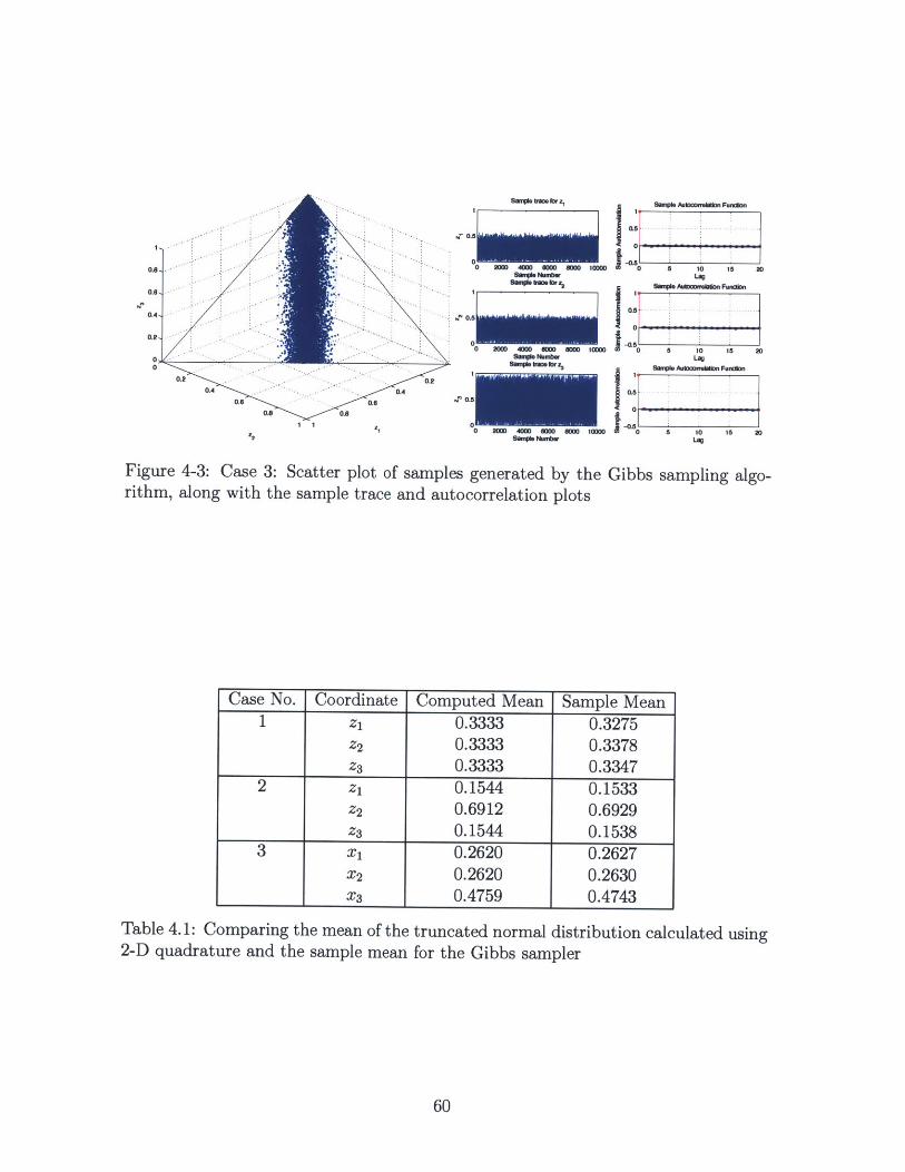
' 0.8

0 = 4OD a=D aO m 1010

S-f' SW~WOWZ

4'40

4'0.

SMPi. NumtwSmqi.w fo.*r z3

I I

- M.A~W

&WO*i A*=fWeab, Fundkln

0i: 0 1 2

Lag

Saipe PAviWws~bn Funm~w

Lagj SmWO9 AuMkiwwtdn Funob,

0s 8 1 :0 15 2D

Figure 4-3: Case 3: Scatter plot of samples generated by the Gibbs sampling algo-rithm, along with the sample trace and autocorrelation plots

Case No. Coordinate Computed Mean Sample Mean1 zi 0.3333 0.3275

Z2 0.3333 0.3378Z3 0.3333 0.3347

2 z1 0.1544 0.1533Z2 0.6912 0.6929Z3 0.1544 0.1538

3 X1 0.2620 0.2627X2 0.2620 0.2630X3 0.4759 0.4743

Table 4.1: Comparing the mean of the truncated normal distribution calculated using2-D quadrature and the sample mean for the Gibbs sampler

60

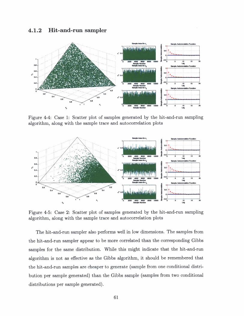
4.1.2 Hit-and-run sampler

Sample KrIWrz

.r 0.1

0 2000 4000 0000 000 WOOD

0.5

0 200 400 0000 000 IOOOoSmple Numb.e0

Sapl 0o.5 z

Sample Aa20melalion Fuln

IK~

I 0 5 10 15 20Logj wo Aamowaeilon Fuwclon

1010 s50

~00Lag

Figure 4-4: Case 1: Scatter plot of samples generated by the hit-and-run samplingalgorithm, along with the sample trace and autocorrelation plots

0 200D 4000 0000 BO00 10000

Smpe Nmr

4'0.5

0 2000 4000 0000 0000 10000

0.5 184f

Saiiple A.*lofwsltiW Funim

0,0 5 10 15 20LagjjSample Aulooowselan Fuadbn

0 5 10 15 20Log


The hit-and-run sampler also performs well in low dimensions. The samples from

the hit-and-run sampler appear to be more correlated than the corresponding Gibbs

samples for the same distribution. While this might indicate that the hit-and-run

algorithm is not as effective as the Gibbs algorithm, it should be remembered that

the hit-and-run samples are cheaper to generate (sample from one conditional distri-

bution per sample generated) than the Gibbs sample (samples from two conditional

distributions per sample generated).

61

1 1 x,

X9

20M 4ow sow a0w8wisk Nrmbrz

0 2000 400 800 4000 D 10000W9M1 w-

Smipie Aatsowu~n Funebmi

i":0 10 2 8D30 4D

Lao, Smiwli AMo~wun FwmaOn

o2io 0 80D 40Lao

SanIple AIW.ooeon Fuwlio

0 10 20 3D 40Lag



Z2 0.3333 0.3250Z3 0.3333 0.3433

2 zi 0.1544 0.1528Z2 0.6912 0.6967Z3 0.1544 0.1505

3 X1 0.2620 0.2687X2 0.2620 0.2682X3 0.4759 0.4631

Table 4.2: Comparing the mean of the truncated normal distribution calculated using2-D quadrature and the sample mean for the hit-and-run sampler

62

Sr~b va f~orz

W-~ 0u.5

'6"~I~z

.2r 0.8

00

Z2

I I

Ir0.8

MOM"

'777777"11i V 11 A LL


.m" w. 1ft;z

r 0.

0 200 000 2000 S 000 1000

I,

emqia ~a~wSmuijd. bms&1rz2

.' 0.8

0 200D 4D 0SW 000 10000ft- ob

Seile A*utierrmiorl Fundn

05 ..... 1..20

S 10 15 20Log

j ne Aumwbw Fundon

Lag9WOgi PAmuow.~Io Fudnon

-Ua 0 5 1:0 18 20Log

Figure 4-7: Case 1: Scatter plot of samples generated by the directional independencesampler, along with the sample trace and autocorrelation plots

Sam* o bmr z

0 200 80 6 0 8000 10D0

10.. 017" 1177 I

Swoe Au8Worekmn Fundion

0 10 18 20Lag

9W"Autioreblion Fundion

0 1 15 20Logj pe Auiwwekn FndIon

8 10 15 20Lag

Figure 4-8: Case 2: Scatter plot of samples generated by the directional independencesampler, along with the sample trace and autocorrelation plots

The directional independence sampler performs reasonably well in all three test

cases. In the first two cases, the samples appear to be less correlated than the corre-

sponding hit-and-run samples for the same target distribution. In the third example,

the directional sampler performs significantly worse (in terms of autocorrelation). It

is worth noting that the acceptance ratio 1 in the first two cases is around 60 percent,

while the acceptance ratio in the third case is around 10 percent. This indicates that

'Acceptance ratio = (number of samples accepted in accept-reject step)/(total number of samples)

63

1 1

Z2

0

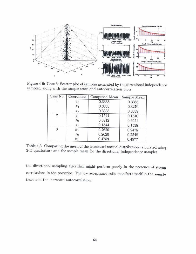
LaoC anp49 AugiawuIoo FuialO~n

04 10 2 3D 40

Figure 4-9: Case 3: Scatter plotsampler, along with the sample

Table 4.3: Comparing the mean2-D quadrature and the sample

of samples generated by the directional independencetrace and autocorrelation plots

of the truncated normal distribution calculated usingmean for the directional independence sampler

the directional sampling algorithm might perform poorly in the presence of strong

correlations in the posterior. The low acceptance ratio manifests itself in the sample

trace and the increased autocorrelation.

64

aIn= 0=uit


Z2 0.3333 0.3276Z3 0.3333 0.3339

2 zi 0.1544 0.1540Z2 0.6912 0.6921Z3 0.1544 0.1538

3 X1 0.2620 0.2475X2 0.2620 0.2548X3 0.4759 0.4977

Sepoe bum fDr j

4.2 Feed reconstruction example

To test our Bayesian model, we applied this algorithm to a feed reconstruction prob-

lem on a real dataset from a plant. Detailed measurements of some sample feedstock

in terms of pseudo-compounds were collected in a laboratory setting. The objective

of the feed reconstruction is to use these detailed measurements along with some

bulk concentrations and rapid distillation analysis of some unknown feedstock in the

refinery to infer the detailed composition of the unknown feedstock in terms of the

pseudo-compounds.

The Bayesian model is applied to this problem and the posterior truncated Gaus-

sian mean and covariance parameters are derived.To explore this high-dimensional

posterior distribution, we attempt to use the three sampling algorithms that were

proposed in the previous section. The presence of high posterior correlations coupled

with the large dimensionality of the problem makes this a difficult distribution to

analyze.

Among the three algorithms, only the Gibbs sampler manages to scale with the

number of dimensions and produce reasonable results. The hit-and-run sampler and

the directional independence sampler produce poorly mixing chains even with an

extremely large number of samples. This tells us that while the hit-and-run and di-

rectional independence sampler produce reasonable results in low-dimensions, they do

not scale well with the number of dimensions, and in the presence of high correlations

(as in the feed reconstruction case), become ineffective. Thus, the Gibbs sampler is

used to sample the posterior distribution of the Bayesian model.

Figure (TODO) shows the sample trace along 2 particular coordinates for the

Gibbs samples generated from the truncated normal posterior distribution, and its

corresponding autocorrelation. It can be observed that along some dimensions, the

autocorrelation in the samples is very large. This is one of the main drawbacks of

using the Gibbs sampler, and requires generating a large number (~ millions ) of

samples to overcome the heavy correlation.

Figure (4-11) shows the marginal densities of pseudocomponents that belong to

65

0.107OM 0.6

8a.l0.l'8~08.. 1100 6 10 IS 20 20 30 36 40 45 0

0.8

0.4

0.2

.00

0 0 1 .5 2 2,5 3 5

Figure 4-10: Sample trace and autocorrelations along selected coordinates in theBayesian feed reconstruction example

2 different reacting families. Instead of a single "best" concentration, the Bayesian

model produces a distribution over a range of possible concentrations. The width

of these marginal densities provides an idea of the uncertainty associated with the

concentration of the particular pseudo-compound.

The Bayesian model allows us to understand the impact of the measured bulk

properties on the uncertainty of the concentrations of the pseudo-compounds. To

illustrate this, consider the following example. In figure (4-12), the histogram on the

left shows the marginal posterior densities of the pseudo-compounds in a particu-

lar nitrogen containing family. When the measured bulk nitrogen concentration is

increased, the uncertainty in the concentrations of the nitrogen containing psuedo-

compounds also increases, which seems reasonable.

Finally, the Bayesian framework provides a fine control on the on the degree-of-

belief in the laboratory and bulk measurements. For example, in figure (4-13), the

marginal densities on the left correspond to a scenario in which the variance associated

66

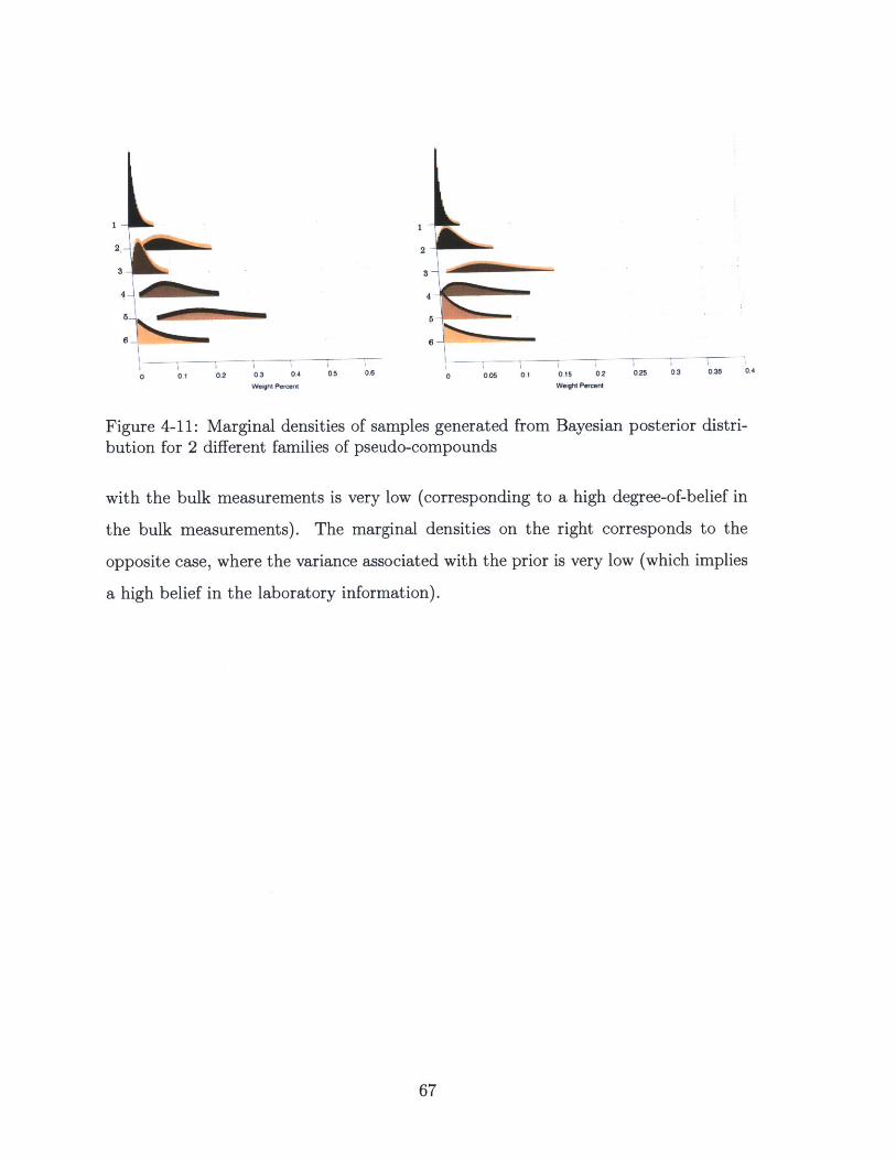
2 -

0 0.1 0.2 03 0.4 0.5 0.6

Weight Percent

2

6

0 0.05 0.1 0.15 02 0,25 0.3 0.35 0.4

Weight Percent

Figure 4-11: Marginal densities of samples generated from Bayesian posterior distri-bution for 2 different families of pseudo-compounds

with the bulk measurements is very low (corresponding to a high degree-of-belief in

the bulk measurements). The marginal densities on the right corresponds to the

opposite case, where the variance associated with the prior is very low (which implies

a high belief in the laboratory information).

67

ii3

4l

3

4

0.2 0.3 04

WeighN PWCOMt

0,5 0.60 0.1 0.2 0.3 0.4

Weight Percent

0.5 0.6 07

Figure 4-12: Marginal densities of concentrations of pseudo-compounds infamily for varying bulk concentrations

2.-'i 0 -3

0 0.1 02 03 04

Weogt Pecent

0.5 0.6

8

41

0

a particular

005 01 0.15 02 025 03 035 0.4

Weih Peren

0.45

Figure 4-13: Comparing marginal densities of concentrations of pseudo-compoundsin a particular family for varying degrees-of-belief in the bulk and laboratory mea-surements respectively

68

0 0.1 0.8

2 J JI&O

4.3 Summary

In this chapter, we tested the performance of the various samplers that were discussed

in the previous chapter. While all the three samplers produce reasonable results in

low dimensions, only the Gibbs sampler manages to work in high dimensions. Then,

we implemented the Bayesian feed reconstruction algorithm for a real data set from

a plant, and analyzed the resulting posterior distribution using the Gibbs sampler.

69

Chapter 5

Conclusions

In this thesis, we developed a Bayesian inference algorithm for the feed reconstruction

problem. The Bayesian approach addresses some of the shortcomings of current feed

reconstruction schemes in literature, by explicitly incorporating uncertainty into the

reconstruction process.

On the computational front, we reviewed and implemented three different algo-

rithms to sample from the truncated normal posterior distribution that results from

the Bayesian reconstruction algorithm. In lower dimensions, all three algorithms

work satisfactorily.In high dimensions, the hit-and-run and the directional indepen-

dence sampler become ineffective for most applications. The Gibbs sampler produces

samples from the posterior distribution, but these are expensive to compute (since

each sample requires sampling n conditional distributions), and are highly correlated.

The Bayesian reconstruction algorithm coupled with the Gibbs sampler was ap-

plied to study a feed reconstruction example in a real plant scenario. The result-

ing model captured the uncertainty in both the bulk measurements and the prior

information, while providing an intuitive way to tune the degree-of-belief in each

measurement.

We believe that the flexibility of the Bayesian modeling technique, combined with

the elegant handling of uncertainty, makes the Bayesian approach a novel and useful

alternative to current feed reconstruction algorithms.

71

5.1 Future work

The following represents some directions for future study that we believe can be used

to extend the work in this thesis

" While we have presented a complete Bayesian algorithm to reconstruct any

feedstock in the refinery, we are still in the process of validating our ap-

proach. The ideal validation framework would require detailed laboratory

analysis of a feedstock whose bulk measurements are available in the plant.

Then, the detailed analysis from the lab can be compared with the results

from the Bayesian model with the bulk measurements, and the quality of

the reconstruction can be ascertained. However, the complicated and expen-

sive nature of analytical chemistry prohibits the gathering of such validation

data. In the absence of analytical data from the laboratory, a simulation

tool such as Aspen HYSYS can be used to simulate the laboratory mea-

surements (like distillation analysis and bulk concentrations) of some known

mixture of pseudo-compounds. Then, the detailed analysis can be used in

the feed reconstruction procedure, and the inferred concentration distribu-

tions can be compared with the known detailed composition.

" In the construction of the likelihood, we assumed that the bulk properties

that were measured in the plant could be obtained as a linear function of

the weight fractions of the psuedo-compounds. While this is true for a large

class of bulk properties that are measured in the refinery, the procedure

can still be extended to properties that are related to the weight fractions

in a nonlinear fashion. The resulting posterior distribution will not be a

truncated normal distribution, and any subsequent analysis will require the

use of sophisticated sparse quadrature or sampling techniques.

" In the current feed reconstruction scheme, we assumed that the parameters

of the gamma distribution that are estimated from laboratory data are

constant. This assumption is not necessary, and can be relaxed by assuming

72

that the parameters are random. This idea is referred to as a fully Bayesian

approach to modeling. The fully Bayesian feed reconstruction model is

discussed in appendix A.

9 The Gibbs sampling algorithm functions as a reasonable technique to gen-

erate samples from high dimensional posterior distributions. However, the

algorithm scales very poorly with the number of dimensions, and becomes

very slow for high dimensional problems, which are common in feed re-

construction settings. The Gibbs algorithm is very general, and does not

leverage many properties of the simplex, such as linearity and convexity.

We developed the directional independence sampler to take advantage of

some of these properties, but it does not appear to scale well with the

number of dimensions thanks to the phenomenon of measure concentration.

We believe that the structure of the simplex combined with the Gaussian

nature of the distribution allows for a good sampler, that can generate al-

most independent samples as the dimensionality of the problem rises. A fast

sampling algorithm is important to the practical application of the Bayesian

approach, both in the context of feed reconstruction and general chemical

systems.

73

Appendix A

Fully Bayesian procedure

In the Bayesian feed reconstruction mode, the parameters of the gamma distribution

were estimated using an MLE approach. An alternative approach would be to as-

sume that the parameters of the gamma distribution themselves are random, with

their probability distribution parametrized by hyperparameters. Then, instead of in-

ferring just the weight percents, the parameters of the gamma distribution can also

be inferred jointly. This type of model is sometimes called a fully Bayesian approach

to modeling.

Let i denote the vector of parameters of the gamma distribution corresponding

to the i-th family. Then, using the same notation as chapter 2, the Bayes equation

in this case can be rewritten as

p(Y, @|D,) oc L(D,|Y, @)p(Y|@)p(@) (A.1)

To finally obtain obtain a posterior distribution on Y, the joint posterior distri-

bution from equation (A.1) has to be marginalized over 4:

p(Y|D,) oc Jp(Y,@|1Dp)d@' (A.2)

The fully Bayesian version of feed reconstruction is the most general Bayesian

framework to analyze the feed reconstruction problem, and our preceding discussion

in the body of this thesis can be seen as a special case of this approach.

75

Appendix B

Restriction of a Gaussian to a line

Given a point x E S C R" , and a direction d c R" (note that lid| =- 1), let us suppose

we are interested in restricting the Gaussian NA(p, E), truncated on the set S along

the line y = x + Ad, where A E {A E Rly E S} 1.

p(x + Ad) = |El--0 5 (27r)-n/ 2 exp(-(x + Ad - I)TE-1(x + Ad - p)/2)

oc exp(-(x - p + Ad)TE' (x - p + Ad)/2)

oc exp((-(x - p)TE-l(x - p - A2dT7E-d + 2A(x - p)T E-ld)/2)

oc exp((-A 2dTE- d + 2A(x - p)TE-1d)/2) {-.- (x - p) constant along d}

c exp(-(A - A)2/(2& 2 )) {Completing the square in A}

where

A~~d (X_ -)1d

2 1

dTE-ld

This implies that A - (/t, (,2). Furthermore, if A is truncated, such that A E

[a, b], we can evaluate p(A) by using a standard transformation. First, we write

h A int z

'This implies that A might belong to an interval

77

where z is the standard normal random variable. Then, z is truncated to the set

[c, e] = [(a - P'))/a, (b - P')/6]. This makes simulation and density evaluation much

cheaper. Since we are simulating from the truncated standard normal distribution,

there are several fast algorithms and packages that can be employed. The density of

A truncated to [a, b] can be computed as

p(Ald) =<b(e) - <b(c)

where # and <} denote the probability and cumulative distribution functions of the

standard normal distribution. There are fast algorithms available to compute the

probability and cumulative densities [26].

78

Appendix C

Projected Normal Distribution

Directional statistics is a branch of statistics that is used to understand and model

random directional data. While traditional random variables are often modeled over

R", directional data are defined only over the unit sphere. This basic difference pro-

motes a slightly different approach to understanding statistics over spheres. Popular

measures of central tendency are still applicable to spherical data, but they are often

handled with slight modifications.

One particular measure of interest is the mean. For example, let x 1, X2,... X,

represent n points on the unit sphere in p dimensions. Then, their sample mean is

given by

S= - xi (C.1)i=1

Then, we define the mean resultant length, p = ||2|| E [0, 1) and the mean resultant

direction t = t/p.

Like the mean, we can also define different measures of central tendency to direc-

tional data, but it is out of the scope of this work. For a comprehensive treatment of

directional statistics, the reader is referred to [25].

The projected normal distribution is a convenient distribution that can be used

to model directional data. In n - m-dimensions, we may denote the unit sphere

as Sn-m-1, which is a subset of R"-m . If we have x ~ K(p, E) C R" m , and

define u = x/||x112 , then u is said to be distributed as a projected n - m-variate

79

normal random variable, denoted as u ~ PN,(p, E) [25] (It should be noted that the

parameters y and E cannot be uniquely identified, since taking ap and a2 E does not

alter the distribution of directions [31], but we can address this problem by requiring

det(E) = 1). Pukkila et al. [33] provide a closed form expression for the pdf of u with

respect to the surface element on the p-dimensional unit sphere dw, as

p(Ulp, E) = |27rYi/23P/2I(Q2Q31/ 2)exp [-2 1 (Q1 - Q2/Q3)] (C.2)

where Q1 - pt -A, Q2 = - Y, Q3 y ly

and

ja r-lexp (r - a) 2 dr

While this integral may be hard to evaluate, Pukkila et al. suggest using the recursive

relation

Ip(C) (p - 1)I,- 2 (a) + aI,-(a) p > 2

with the initial values

I2(a) e~2 /2 + a1l(a), 1(a) = v 27<b(a)

Let us study the effect of varying the parameters of the projected normal distri-

bution. The scalar parameter ||t| serves as a measure of concentration on the unit

sphere. To highlight this property of I|p|, 4 different examples are considered in figure

(C-1), with increasing values of ||pl|, while maintaining the same direction of P.

Increasing the value of ||p|| causes the samples generated from the projected nor-

mal distribution to cluster. If we denote the mean resultant length of the samples as

p, then it can be empirically observed that p increases with an increase in p. This sug-

gests a relationship between |1ti| and p, which was discovered by Presnell et al. [31],

as

_____ 2/ (C.3)M 1 d 2)pV (d+2M 2' 2 + l2-

80

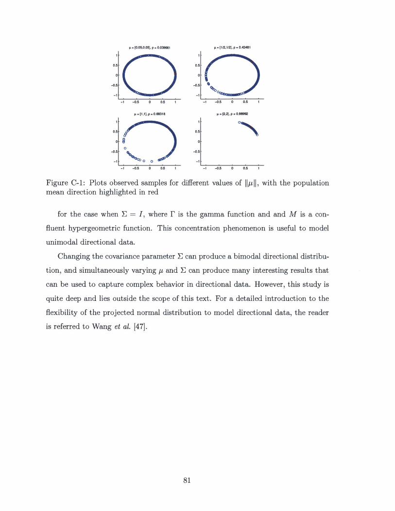
Is - [0.05,0.05], p - 0.039661 s - [1/2,M12], p - 0.43481

0(10.5

0

-0.5

-1

-1 -0.5 0 0.5 1

p1 1,1], p -0.68318

0.6

-0.5.

..1 o o0

-1 -0.5 0 0.5 1

I

0.5

0

-0.5

-1

-1 -0.5 0 0.5 1

s - [2,2], p 0.9892

0.5

0

-0.5

-1

-1 -0.5 0 0.5 1

Figure C-1: Plots observed samples for different values of ||p||, with the populationmean direction highlighted in red

for the case when E = I, where F is the gamma function and and M is a con-

fluent hypergeometric function. This concentration phenomenon is useful to model

unimodal directional data.

Changing the covariance parameter E can produce a bimodal directional distribu-

tion, and simultaneously varying L and E can produce many interesting results that

can be used to capture complex behavior in directional data. However, this study is

quite deep and lies outside the scope of this text. For a detailed introduction to the

flexibility of the projected normal distribution to model directional data, the reader

is referred to Wang et al. [47].

81

Bibliography

[1] CS294-13: Special Topics in Advanced Computer Graphics.http://inst.eecs.berkeley.edu/ cs294-13/fa09/lectures/scribe-lecture4.pdf.Accessed: 12/12/2012.

[2] Milton Abramowitz and Irene A Stegun. Handbook of mathematical functionwith formulas, graphs, and mathematical tables. National Bureau of Standsards,Applied Mathematics Series, 55, 1970.

[3] James H Albert and Siddhartha Chib. Bayesian analysis of binary and poly-chotomous response data. Journal of the American statistical Association,88(422):669-679, 1993.

[4] Ioannis P Androulakis, Mark D Weisel, Chang S Hsu, Kuangnan Qian, Larry AGreen, John T Farrell, and Kiyomi Nakakita. An integrated approach for creatingmodel diesel fuels. Energy & fuels, 19(1):111-119, 2005.

[5] Alenxander Barvinok. Lecture notes on measure concentration.http://www.math.lsa.umich.edu/ barvinok/total710.pdf, 2005.

[6] C.J.P. Belisle, H.E. Romeijn, and Robert L. Smith. Hit-and-run algorithmsfor generating multivariate distributions. Mathematics of Operations Research,18(2):255-266, 1993.

[7] D.P. Bertsekas and J.N. Tsitsiklis. Introduction to probability, volume 1. AthenaScientific Nashua, NH, 2002.

[8] Steve Brooks, Andrew Gelman, Galin Jones, and Xiao-Li Meng. Handbook ofMarkov Chain Monte Carlo. Chapman and Hall/CRC, 2011.

[9] Darin M Campbell and Michael T Klein. Construction of a molecular represen-tation of a complex feedstock by monte carlo and quadrature methods. AppliedCatalysis A: General, 160(1):41-54, 1997.

[10] M.H. Chen and B.W. Schmeiser. General hit-and-run monte carlo sampling forevaluating multidimensional integrals. Operations Research Letters, 19(4):161-169, 1996.

[11] Nicolas Chopin. Fast simulation of truncated gaussian distributions. Statisticsand Computing, 21(2):275-288, 2011.

83

[12] ASTM Subcommittee D02.08. D86 Standard Test Method for Distillation ofPetroleum Products at Atmospheric Pressure. ASTM International, 28th edition,2012.

[13] N Dobigeon and JY Tourneret. Efficient sampling according to a multivariategaussian distribution truncated on a simplex. Technical report, ENSEEIHT,2007.

[14] Jo Eidsvik and HAkon Tjelmeland. On directional metropolis-hastings algo-rithms. Statistics and Computing, 16(1):93-106, 2006.

[15] B Fleury. Concentration in a thin euclidean shell for log-concave measures.Journal of Functional Analysis, 259(4):832-841, 2010.

[16] A.E. Gelfand and A.F.M. Smith. Sampling-based approaches to calculatingmarginal densities. Journal of the American statistical association, 85(410):398-409, 1990.

[17] J. Geweke. Efficient simulation from the multivariate normal and student-t dis-tributions subject to linear constraints and the evaluation of constraint proba-bilities. In Computing science and statistics: proceedings of the 23rd symposiumon the interface, pages 571-578. Fairfax, Virginia: Interface Foundation of NorthAmerica, Inc, 1991.

[18] W.R. Gilks, S. Richardson, and D. Spiegelhalter. Markov Chain Monte Carlo inpractice: interdisciplinary statistics, volume 2. Chapman & Hall/CRC, 1995.

[19] D Hudebine, J Verstraete, and T Chapus. Statistical reconstruction of gasoil cuts. Oil & Gas Science and Technology-Revue dIFP Energies nouvelles,66(3):461-477, 2009.

[20] D.P. Kroese, T. Taimre, and Z.I. Botev. Handbook of Monte Carlo Methods,volume 706. Wiley, 2011.

[21] Richard A Levine, Zhaoxia Yu, William G Hanley, and John J Nitao. Imple-menting random scan gibbs samplers. Computational Statistics, 20(1):177-196,2005.

[22] Genyuan Li and Herschel Rabitz. A general analysis of exact lumping in chemicalkinetics. Chemical engineering science, 44(6):1413-1430, 1989.

[23] Dimitris K Liguras and David T Allen. Structural models for catalytic cracking.1. model compound reactions. Industrial & Engineering Chemistry Research,28(6):665-673, 1989.

[24] J.S. Liu. Monte Carlo strategies in scientific computing. Springer, 2008.

[25] Kanti V Mardia and Peter E Jupp. Directional statistics, volume 494. Wiley,2009.

84

[26] George Marsaglia. Evaluating the normal distribution. Journal of StatisticalSoftware, 11(4):1-7, 2004.

[27] Mi Mi Saine Aye and Nan Zhang. A novel methodology in transforming bulkproperties of refining streams into molecular information. Chemical engineeringscience, 60(23):6702-6717, 2005.

[28] Brian Neelon and David B Dunson. Bayesian isotonic regression and trend anal-ysis. Biometrics, 60(2):398-406, 2004.

[29] Matthew Neurock, Abhash Nigam, Daniel Trauth, and Michael T Klein. Molec-ular representation of complex hydrocarbon feedstocks through efficient charac-terization and stochastic algorithms. Chemical engineering science, 49(24):4153-4177, 1994.

[30] Ari Pakman and Liam Paninski. Exact hamiltonian monte carlo for truncatedmultivariate gaussians. arXiv preprint arXiv:1208.4118, 2012.

[31] Brett Presnell and Pavlina Rumcheva. The mean resultant length of the spheri-cally projected normal distribution. Statistics & Probability Letters, 78(5):557-563, 2008.

[32] W.H. Press, S.A. Teukolsky, W.T. Vetterling, and B.P. Flannery. Numericalrecipes in C: the art of scientific computing. 2. Cambridge: CUP, 1992.

[33] Tarmo M Pukkila and C Radhakrishna Rao. Pattern recognition based on scaleinvariant discriminant functions. Information sciences, 45(3):379-389, 1988.

[34] Steven P Pyl, Zhen Hou, Kevin M Van Geem, Marie-Frangoise Reyniers, Guy BMarin, and Michael T Klein. Modeling the composition of crude oil fractionsusing constrained homologous series. Industrial & Engineering Chemistry Re-search, 50(18):10850-10858, 2011.

[35] Steven P Pyl, Kevin M Van Geem, Marie-Frangoise Reyniers, and Guy B Marin.Molecular reconstruction of complex hydrocarbon mixtures: An application ofprincipal component analysis. AIChE Journal, 56(12):3174-3188, 2010.

[36] Christian P Robert and George Casella. Monte Carlo statistical methods.Springer, 2004.

[37] C.P. Robert. Simulation of truncated normal variables. Statistics and computing,5(2):121-125, 1995.

[38] G. Rodriguez-Yam, R.A. Davis, and L.L. Scharf. Efficient gibbs sampling oftruncated multivariate normal with application to constrained linear regression.2004.

[39] S Roweis. Gaussian identities. 1999.

85

[40] Sam Roweis and Zoubin Ghahramani. A unifying review of linear gaussian mod-els. Neural computation, 11(2):305-345, 1999.

[41] Devinder S Sivia. Data analysis: a Bayesian tutorial. Oxford University Press,1996.

[42] Robert L. Smith. Efficient monte carlo procedures for generating points uniformlydistributed over bounded regions. Operations Research, 32(6):1296-1308, 1984.

[43] Alan D Sokal. Monte carlo methods in statistical mechanics: foundations andnew algorithms, 1989.

[44] Daniel M Trauth, Scott M Stark, Thomas F Petti, Matthew Neurock, andMichael T Klein. Representation of the molecular structure of petroleum residthrough characterization and monte carlo modeling. Energy & fuels, 8(3):576-580, 1994.

[45] Kevin M Van Geem, Damien Hudebine, Marie Francoise Reyniers, FrancoisWahl, Jan J Verstraete, and Guy B Marin. Molecular reconstruction of naphthasteam cracking feedstocks based on commercial indices. Computers & chemicalengineering, 31(9):1020-1034, 2007.

[46] Jan J Verstraete, Nadege Revellin, Hugues Dulot, and Damien Hudebine. Molec-ular reconstruction of vacuum gasoils. Prepr. Pap.-Am. Chem. Soc., Div. FuelChem, 49(1):20, 2004.

[47] Fangpo Wang and Alan E Gelfand. Directional data analysis under the generalprojected normal distribution. Statistical Methodology, 2012.

[48] Larry Wasserman. All of statistics: a concise course in statistical inference.Springer Verlag, 2004.

[49] Curtis H Whitson, Thomas F Anderson, and Ingolf Soreide. Application ofthe gamma distribution model to molecular weight and boiling point data forpetroleum fractions. Chemical engineering communications, 96(1):259-278, 1990.

[50] Yongwen Wu and Nan Zhang. Molecular characterization of gasoline and dieselstreams. Industrial & Engineering Chemistry Research, 49(24):12773-12782,2010.

86

A Bayesian approach to feed reconstruction

Documents

Transcript of A Bayesian approach to feed reconstruction