A basic Michelson laser interferometer for the undergraduate teaching laboratorydemonstrating picometer sensitivityKenneth G. Libbrecht and Eric D. Black Citation: American Journal of Physics 83, 409 (2015); doi: 10.1119/1.4901972 View online: http://dx.doi.org/10.1119/1.4901972 View Table of Contents: http://scitation.aip.org/content/aapt/journal/ajp/83/5?ver=pdfcov Published by the American Association of Physics Teachers Articles you may be interested in Characterization of a Piezoelectric Buzzer Using a Michelson Interferometer Phys. Teach. 48, 610 (2010); 10.1119/1.3517032 Using a Michelson Interferometer to Measure Coefficient of Thermal Expansion of Copper Phys. Teach. 47, 306 (2009); 10.1119/1.3116844 Instantaneous multiple use of Michelson's interferometer Phys. Teach. 44, 314 (2006); 10.1119/1.2195408 Modified Michelson fiber-optic interferometer: A remote low-coherence distributed strain sensor array Rev. Sci. Instrum. 74, 270 (2003); 10.1063/1.1525867 Mechanical resonance detected with a Michelson interferometer Am. J. Phys. 65, 441 (1997); 10.1119/1.18558

This article is copyrighted as indicated in the article. Reuse of AAPT content is subject to the terms at: http://scitation.aip.org/termsconditions. Downloaded to IP:

131.215.70.231 On: Thu, 14 May 2015 21:54:36

A basic Michelson laser interferometer for the undergraduate teachinglaboratory demonstrating picometer sensitivity

Kenneth G. Libbrechta) and Eric D. Blackb)

264-33 Caltech, Pasadena, California 91125

(Received 3 July 2014; accepted 4 November 2014)

We describe a basic Michelson laser interferometer experiment for the undergraduate teaching

laboratory that achieves picometer sensitivity in a hands-on, table-top instrument. In addition to

providing an introduction to interferometer physics and optical hardware, the experiment also

focuses on precision measurement techniques including servo control, signal modulation,

phase-sensitive detection, and different types of signal averaging. Students examine these

techniques in a series of steps that take them from micron-scale sensitivity using direct fringe

counting to picometer sensitivity using a modulated signal and phase-sensitive signal averaging. After

students assemble, align, and characterize the interferometer, they then use it to measure nanoscale

motions of a simple harmonic oscillator system as a substantive example of how laser interferometry

can be used as an effective tool in experimental science. VC 2015 American Association of Physics Teachers.

[http://dx.doi.org/10.1119/1.4901972]

I. INTRODUCTION

Optical interferometry is a well-known experimental tech-nique for making precision displacement measurements,with examples ranging from Michelson and Morley’s famousaether-drift experiment to the extraordinary sensitivity ofmodern gravitational-wave detectors. By carefully managinga variety of fundamental and technical noise sources, dis-placement sensitivities of better than 10�19 m/Hz �1=2 havebeen demonstrated (roughly 10�13 wavelengths of light).1,2

Given the widespread use of interferometric measurementtechniques in experimental science, we sought to construct afairly basic, yet high-precision, Michelson interferometer foruse in our undergraduate teaching laboratory. Students in thecourse would likely have no previous background in opticsor interferometry, and our goals for this project included fourneeds. First, we wanted to produce a compact instrumentthat gives students hands-on experience with optical andlaser hardware, including optical alignment. Second, wewanted to use a minimal optical layout to reduce complexityand cost. Third, we wanted to provide a brief but nontrivialintroduction to modern measurement techniques, includingservo control, signal modulation, phase-sensitive detection,and different types of signal averaging. Fourth, we wanted todemonstrate the highest displacement sensitivity that is prac-tically achievable without enshrouding the instrumentbeneath layers of acoustic and seismic isolation.

A literature search quickly revealed an enormous selectionof potentially relevant references describing the multitudeof uses of laser interferometry for a broad range of measure-ments. Given our goals, however, we soon turned our atten-tion away from many papers describing low-sensitivityinterferometry, including the basic fringe-counting Michelsoninterferometers that have been used for many years in teach-ing labs to measure, for example, the indices of refraction ofgases or thermal expansion coefficients.3–7

One also encounters numerous examples in the literature oflaser interferometers demonstrating picometer sensitivity usinginstruments of greater complexity than the basic Michelson,requiring some combination of additional optical elements,more elaborate optical layouts, frequency-modulated lasers,frequency-shifting acousto-optical modulators, homodyne or

heterodyne readouts, and perhaps multiple lasers.8–14 Moderninterferometry review articles tend to focus on complex opticalconfigurations as well,15 as they offer improved sensitivity andstability over simpler designs. While these advanced instru-ment strategies are becoming the norm in research and indus-try, for educational purposes we sought to develop a basicMichelson interferometer that uses the archetypal optical lay-out often found in textbooks, and we found that these advancedtechniques were not compatible with our objectives.

We soon narrowed our literature search to precision dis-placement measurements using basic (single-beam)Michelson interferometers.16–18 Precision interferometry iscertainly not a new subject, and these references describeinterferometers that are similar to the one we describe below.During the building phase of our project, however, we soonfound that many experimental details not provided in ourreferences were quite critical for achieving picometer sensi-tivity. These include the choice of optical components andmounting hardware, optical alignment specifics, unwantedmechanical resonances, servo design, managing seismic andacoustic noise, and devising suitable measurement strategies.We generally found that these specifics were difficult to findin the literature, being dispersed over many sources if theycould be found at all. In an attempt to remedy this situation,we describe below the construction and characterization of abasic Michelson interferometer in some detail, and we focusas well on its use in the instructional laboratory.

Our final instrument is designed for physics teaching. It isvisual and tactile, relatively easy to understand, and gener-ally fun to work with, making it well suited for training stu-dents. It demonstrates precision physical measurementtechniques in a compact apparatus with a simple opticallayout. Students place some of the optical components them-selves and then align the interferometer, thus gaininghands-on experience with optical and laser hardware. Thealignment is straightforward but not trivial, and the variousinterferometer signals are directly observable on the oscillo-scope. Some features of the instrument include:16–18 (1) pie-zoelectric control of one mirror’s position, allowing precisecontrol of the interferometer signal, (2) the ability to lock theinterferometer at its most sensitive point, (3) the ability tomodulate the mirror position while the interferometer is

409 Am. J. Phys. 83 (5), May 2015 http://aapt.org/ajp VC 2015 American Association of Physics Teachers 409

This article is copyrighted as indicated in the article. Reuse of AAPT content is subject to the terms at: http://scitation.aip.org/termsconditions. Downloaded to IP:

131.215.70.231 On: Thu, 14 May 2015 21:54:36

locked, thus providing a displacement signal of variablemagnitude and frequency, and (4) phase-sensitive detectionof the modulated displacement signal, both using the digitaloscilloscope and using basic analog signal processing.

In working with this experiment, students are guidedthrough a series of measurement strategies, from micron-scale measurement precision using direct fringe countingto picometer precision using a modulated signal and phase-sensitive signal averaging. The end result is the ability tosee displacement modulations below one picometer in a10-cm-long interferometer arm, which is like measuring thedistance from New York to Los Angeles with a sensitivitybetter than the width of a human hair.

Once the interferometer performance has been explored,students then incorporate a magnetically driven oscillatingmirror in the optical layout.21 Observation and analysis ofnanometer-scale motions of the high-Q oscillator revealseveral aspects of its behavior, including: (1) the near-resonant-frequency response of the oscillator, (2) mass-dependent frequency shifts, (3) changes in the mechanical Qas damping is added, and (4) the excitation of the oscillatorvia higher harmonics using a square-wave drive signal.

With this apparatus, students learn about optical hardwareand lasers, optical alignment, laser interferometry, piezoelec-tric transducers, photodetection, electronic signal processing,signal modulation to avoid low-frequency noise, signal aver-aging, and phase-sensitive detection. Achieving a displace-ment sensitivity of 1/100th of an atom with a table-topinstrument provides an impressive demonstration of thepower of interferometric measurement and signal-averagingtechniques. Further quantifying the behavior of a mechanicaloscillator executing nanoscale motions shows the effective-ness of laser interferometry as a measurement tool in experi-mental science.

II. INTERFEROMETER DESIGN AND

PERFORMANCE

Figure 1 shows the overall optical layout of the con-structed interferometer. The 12.7-mm-thick aluminum bread-board (Thorlabs MB1224) is mounted atop a custom-madesteel electronics chassis using rubber vibration dampers, andthe chassis itself rests on rubber feet. The rubber dampersare all approximately 25 mm in size (length and diameter)with 50 A durometer. We found that this two-stage seismic

isolation system is adequate for reducing noise in the inter-ferometer signal arising from benchtop vibrations, as long asthe benchtop is not bumped or otherwise unnecessarily per-turbed. This is particularly true for the phase-sensitive meas-urements described below, which are done at sufficientlyhigh frequencies that only modest damping of seismic noiseis needed.

The helium-neon laser (Meredith HNS-2P) produces a 2mW linearly polarized (500:1 polarization ratio) 633-nmbeam with a diameter of approximately 0.8 mm, and it ismounted in a pair of custom fixed acrylic holders. Thebeamsplitter (Thorlabs BSW10) is a 1-in.-diameter wedgedplate beamsplitter with a broadband dielectric coating givingroughly equal transmitted and reflected beams. It is mountedin a fixed optical mount (Thorlabs FMP1) connected to apedestal post (Thorlabs RS1.5P8E) fastened to the bread-board using a clamping fork (Thorlabs CF125). Mirrors 1and 2 (both Thorlabs BB1-E02) are mounted in standardoptical mounts (Thorlabs KM100) on the same pedestalposts. Using these stout steel pedestal posts is important forreducing unwanted motions of the optical elements.

We note that while inexpensive diode lasers are oftenadequate for making simple fringe-counting interferometers,in general they are not well suited for precision interferome-try. In our experience, diode lasers have poor beam shapes,can exhibit large frequency jumps, often run multi-mode,and are sensitive to back reflection. As a result, the fringequality of a diode-laser interferometer is often erratic. Incontrast, 633-nm helium-neon lasers typically show a nearlyideal Gaussian mode shape, good frequency stability, and amuch smaller optical bandwidth.

The mirror/PZT consists of a small mirror (12.5-mm diam-eter, 2-mm thick, Edmund Optics 83–483, with an enhancedaluminum reflective coating) glued to one end of a piezoelec-tric stack transducer (PZT) (Steminc SMPAK155510D10),with the other end glued to an acrylic disk in a mirror mount.An acrylic tube surrounds the mirror/PZT assembly forprotection, but the mirror only contacts the PZT stack. Thesurface quality of the small mirror is relatively poor (2–3waves over one cm) compared with the other mirrors, but wefound it is adequate for this task, and the small mass of themirror helps push mechanical resonances of the mirror/PZTassembly to frequencies above 700 Hz.

The photodetector includes a Si photodiode (ThorlabsFDS100) with a 3:6 mm� 3:6 mm active area, held in a

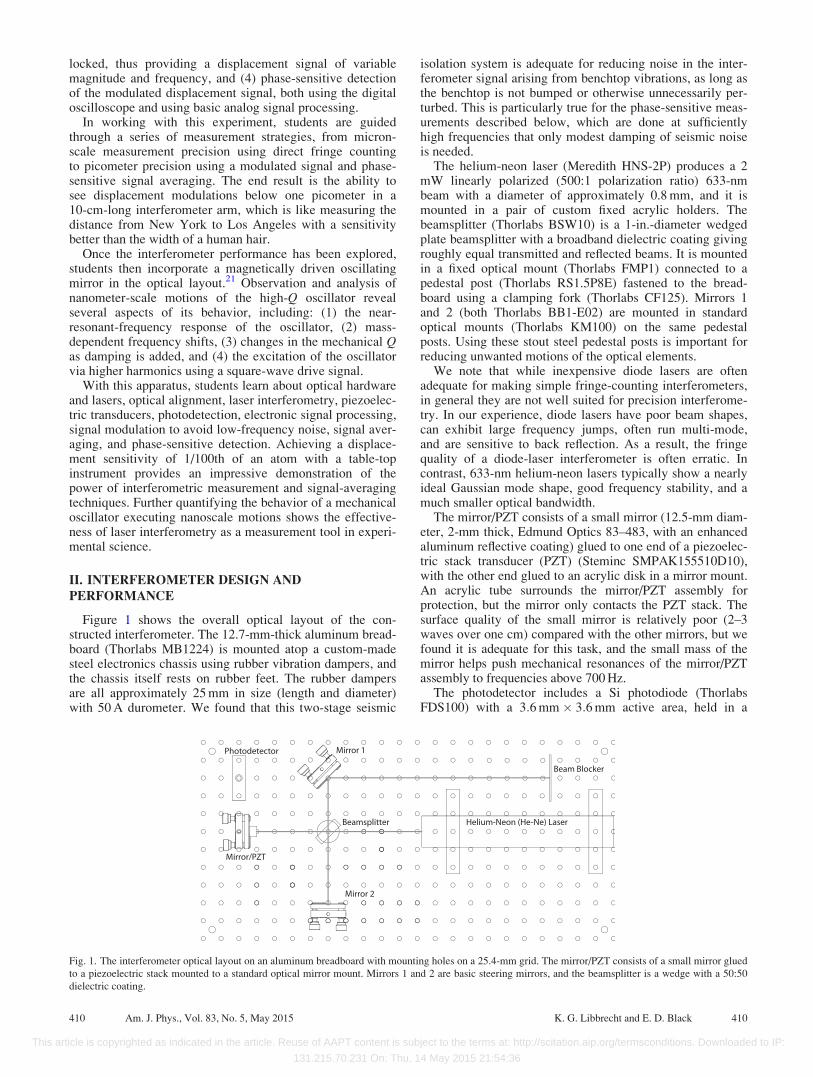
Mirror/PZT

Mirror 1

Mirror 2

Beamsplitter

Photodetector

Helium-Neon (He-Ne) Laser

Beam Blocker

Fig. 1. The interferometer optical layout on an aluminum breadboard with mounting holes on a 25.4-mm grid. The mirror/PZT consists of a small mirror glued

to a piezoelectric stack mounted to a standard optical mirror mount. Mirrors 1 and 2 are basic steering mirrors, and the beamsplitter is a wedge with a 50:50

dielectric coating.

410 Am. J. Phys., Vol. 83, No. 5, May 2015 K. G. Libbrecht and E. D. Black 410

This article is copyrighted as indicated in the article. Reuse of AAPT content is subject to the terms at: http://scitation.aip.org/termsconditions. Downloaded to IP:

131.215.70.231 On: Thu, 14 May 2015 21:54:36

custom acrylic fixed mount. The custom photodiode ampli-fier consists of a pair of operational amplifiers (TL072) thatprovide double-pole low-pass filtering of the photodiodesignal with a 10–ls time constant, as shown in Fig. 4. Theoverall amplifier gain is fixed, giving approximately an 8-Voutput signal with the full laser intensity incident on the pho-todiode’s active area.

The optical layout shown in Fig. 1 was designed toprovide enough degrees of freedom to fully align the inter-ferometer, but no more. The mirror/PZT pointing determinesthe degree to which the beam is misaligned from retroreflect-ing back into the laser (described below), the mirror 2 point-ing allows for alignment of the recombining beams, andthe mirror 1 pointing is used to center the beam on the photo-diode. In addition to reducing the cost of the interferometerand its maintenance, using a small number of optical ele-ments also reduces the complexity of the set-up, improvingits function as a teaching tool.

Three of the optical elements (mirror 1, mirror 2, and thebeamsplitter) can be repositioned on the breadboard orremoved. The other three elements (the laser, photodiode,and the mirror/PZT) are fixed on the breadboard, the onlyavailable adjustment being the pointing of the mirror/PZT.The latter three elements all need electrical connections, andfor these the wiring is sent down through existing holes inthe breadboard and into the electronics chassis below. Theuse of fixed wiring (with essentially no accessible cabling)allows for an especially compact and robust constructionthat simplifies the operation and maintenance of the interfer-ometer. At the same time, the three free elements present stu-dents with a realistic experience placing and aligning laseroptics.

Before setting up the interferometer as in Fig. 1, there area number of smaller exercises students can do with thisinstrument. The Gaussian laser beam profile can beobserved, as well as the divergence of the laser beam. Usinga concave lens (Thorlabs LD1464-A, f¼�50 mm) increasesthe beam divergence and allows a better look at the beamprofile. Laser speckle can also be observed, as well as dif-fraction from small bits of dirt on the optics. Ghost laserbeams from the antireflection-coated side of the beamsplitterare clearly visible, as the wedge in the glass sends thesebeams out at different directions from the main beams.Rotating the beamsplitter 180� results in a different set ofghost beams, and it is instructive to explain these with asketch of the two reflecting surfaces and the resulting inten-sities of multiply reflected beams.

A. Interferometer alignment

A satisfactory alignment of the interferometer is straightfor-ward and easy to achieve, but doing so requires an understand-ing of how real-world optics can differ from the idealized casethat is often presented. As shown in Fig. 2, retroreflecting thelaser beams at the ends of the interferometer arms yields arecombined beam that is sent directly back toward the laser.This beam typically reflects off the front mirror of the laserand reenters the interferometer, yielding an optical cacophonyof multiple reflections and unwanted interference effects.Inserting an optical isolator in the original laser beam wouldsolve this problem, but this is an especially expensive opticalelement that is best avoided in the teaching lab.

The preferred solution to this problem is to misalign thearm mirrors slightly, as shown in Fig. 2. With our

components and the optical layout shown in Fig. 1, misalign-ing the mirror/PZT by 4.3 mrad is sufficient that the initialreflection from the mirror/PZT avoids striking the front mir-ror of the laser altogether, thus eliminating unwanted reflec-tions. This misalignment puts a constraint on the lengths ofthe two arms, however, as can be seen from the second dia-gram in Fig. 2. If the two arm lengths are identical (as in thediagram), then identical misalignments of both arm mirrorscan yield (in principle) perfectly recombined beams that areoverlapping and collinear beyond the beamsplitter. If thearm lengths are not identical, however, then perfect recombi-nation is no longer possible.

The arm length asymmetry constraint can be quantified bymeasuring the fringe contrast seen by the detector. If theposition x of the mirror/PZT is varied over small distances,then the detector voltage can be written

Vdet ¼ Vmin þ1

2Vmax � Vminð Þ 1þ cos 2kxð Þ½ �; (1)

where Vmin and Vmax are the minimum and maximumvoltages, respectively, and k ¼ 2p=k is the wavenumber ofthe laser. This signal is easily observed by sending a trianglewave to the PZT, thus translating the mirror back and forth,while Vdet is observed on the oscilloscope. We define theinterferometer fringe contrast to be

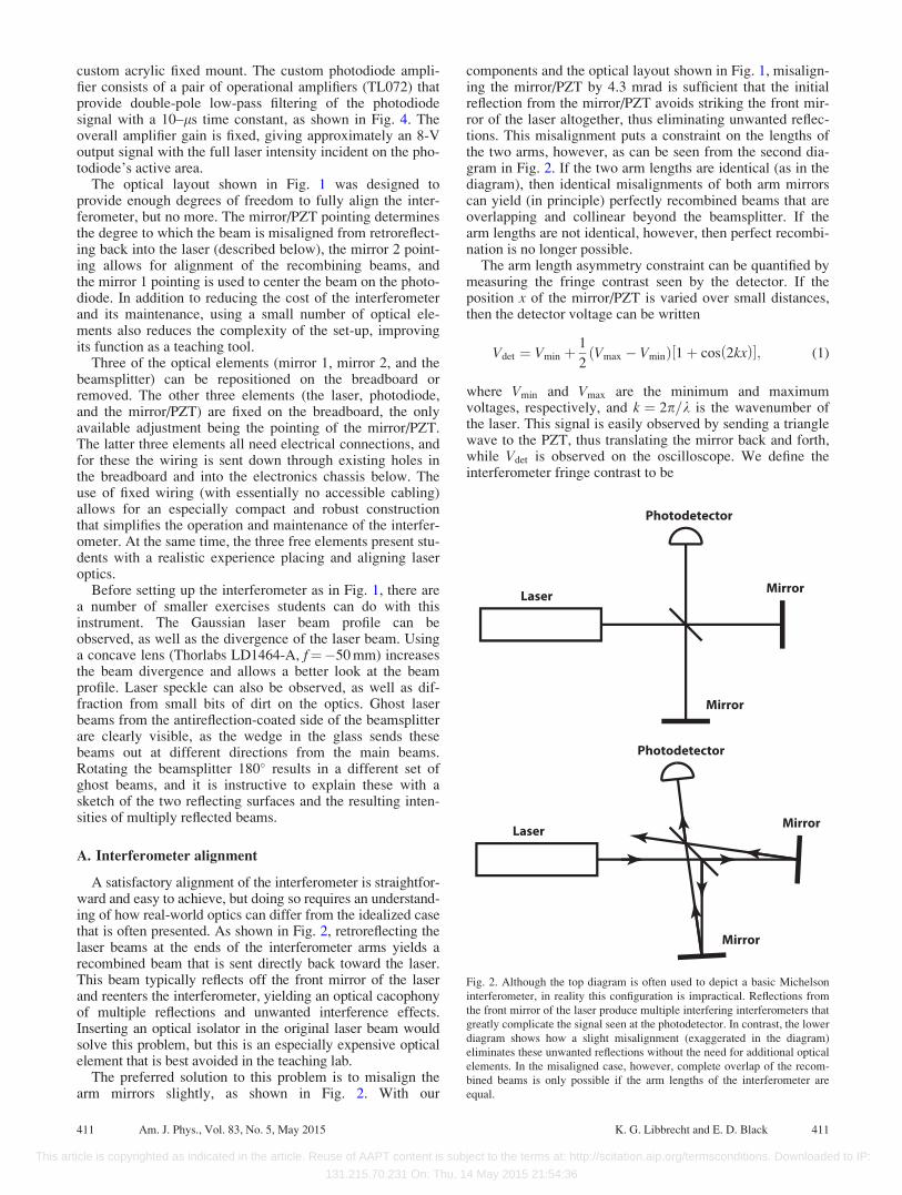
Laser

Photodetector

Photodetector

Laser

Mirror

Mirror

Mirror

Mirror

Fig. 2. Although the top diagram is often used to depict a basic Michelson

interferometer, in reality this configuration is impractical. Reflections from

the front mirror of the laser produce multiple interfering interferometers that

greatly complicate the signal seen at the photodetector. In contrast, the lower

diagram shows how a slight misalignment (exaggerated in the diagram)

eliminates these unwanted reflections without the need for additional optical

elements. In the misaligned case, however, complete overlap of the recom-

bined beams is only possible if the arm lengths of the interferometer are

equal.

411 Am. J. Phys., Vol. 83, No. 5, May 2015 K. G. Libbrecht and E. D. Black 411

This article is copyrighted as indicated in the article. Reuse of AAPT content is subject to the terms at: http://scitation.aip.org/termsconditions. Downloaded to IP:

131.215.70.231 On: Thu, 14 May 2015 21:54:36

FC ¼Vmax � Vmin

Vmax þ Vmin

; (2)

and a high fringe contrast with FC � 1 is desirable forobtaining the best interferometer sensitivity.

With this background, the interferometer alignment con-sists of the following steps. (1) Place the beamsplitter so thereflected beam is at a 90� angle from the original laser beam.The beamsplitter coating is designed for a 90� reflectionangle, plus it is generally good practice to keep the beams ona simple rectangular grid as much as possible. (2) With mirror2 blocked, adjust the mirror/PZT pointing so the reflectedbeam just misses the front mirror of the laser. This is easilydone by observing any multiple reflections at the photodiodeusing a white card. (3) Adjust the mirror 1 pointing so thebeam is centered on the photodiode. (4) Unblock mirror 2and adjust its pointing to produce a single recombined beamat the photodiode. (5) Send a triangle wave signal to the PZT,observe Vdet with the oscilloscope, and adjust the mirror 2pointing further to obtain a maximum fringe contrast FC;max.

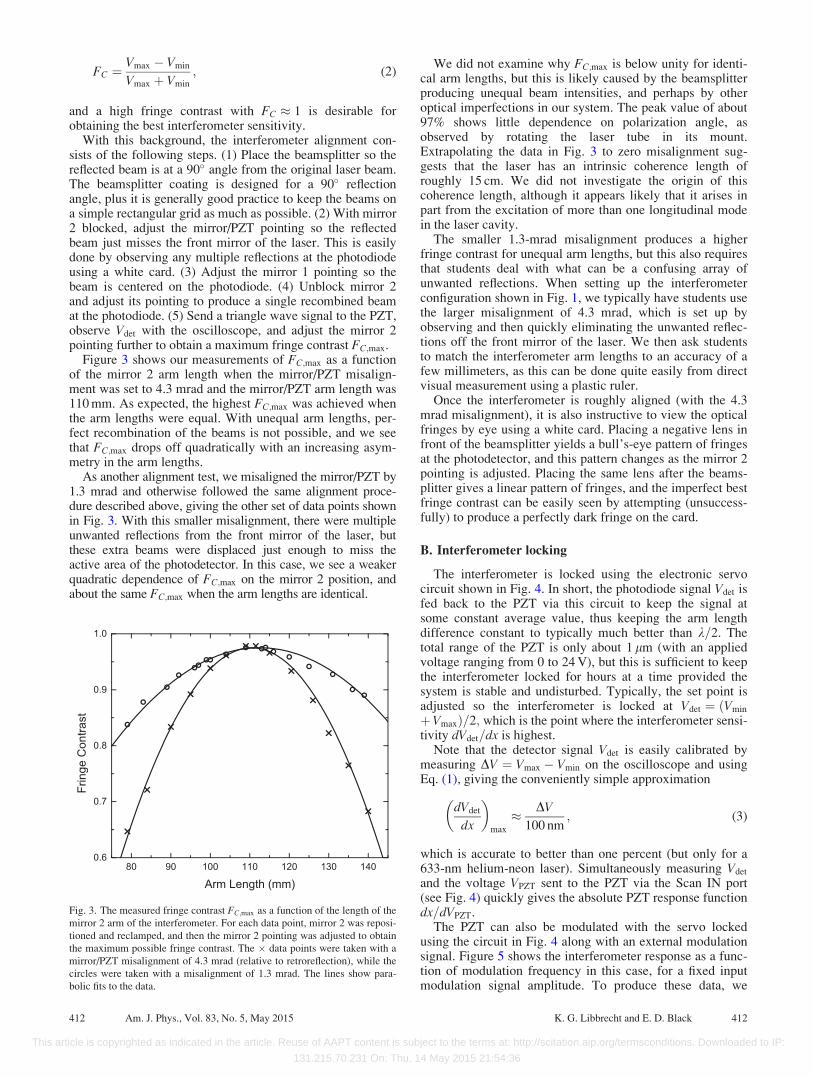
Figure 3 shows our measurements of FC;max as a functionof the mirror 2 arm length when the mirror/PZT misalign-ment was set to 4.3 mrad and the mirror/PZT arm length was110 mm. As expected, the highest FC;max was achieved whenthe arm lengths were equal. With unequal arm lengths, per-fect recombination of the beams is not possible, and we seethat FC;max drops off quadratically with an increasing asym-metry in the arm lengths.

As another alignment test, we misaligned the mirror/PZT by1.3 mrad and otherwise followed the same alignment proce-dure described above, giving the other set of data points shownin Fig. 3. With this smaller misalignment, there were multipleunwanted reflections from the front mirror of the laser, butthese extra beams were displaced just enough to miss theactive area of the photodetector. In this case, we see a weakerquadratic dependence of FC;max on the mirror 2 position, andabout the same FC;max when the arm lengths are identical.

We did not examine why FC;max is below unity for identi-cal arm lengths, but this is likely caused by the beamsplitterproducing unequal beam intensities, and perhaps by otheroptical imperfections in our system. The peak value of about97% shows little dependence on polarization angle, asobserved by rotating the laser tube in its mount.Extrapolating the data in Fig. 3 to zero misalignment sug-gests that the laser has an intrinsic coherence length ofroughly 15 cm. We did not investigate the origin of thiscoherence length, although it appears likely that it arises inpart from the excitation of more than one longitudinal modein the laser cavity.

The smaller 1.3-mrad misalignment produces a higherfringe contrast for unequal arm lengths, but this also requiresthat students deal with what can be a confusing array ofunwanted reflections. When setting up the interferometerconfiguration shown in Fig. 1, we typically have students usethe larger misalignment of 4.3 mrad, which is set up byobserving and then quickly eliminating the unwanted reflec-tions off the front mirror of the laser. We then ask studentsto match the interferometer arm lengths to an accuracy of afew millimeters, as this can be done quite easily from directvisual measurement using a plastic ruler.

Once the interferometer is roughly aligned (with the 4.3mrad misalignment), it is also instructive to view the opticalfringes by eye using a white card. Placing a negative lens infront of the beamsplitter yields a bull’s-eye pattern of fringesat the photodetector, and this pattern changes as the mirror 2pointing is adjusted. Placing the same lens after the beams-plitter gives a linear pattern of fringes, and the imperfect bestfringe contrast can be easily seen by attempting (unsuccess-fully) to produce a perfectly dark fringe on the card.

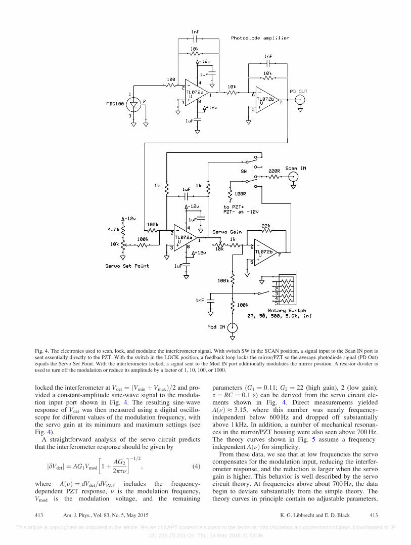
B. Interferometer locking

The interferometer is locked using the electronic servocircuit shown in Fig. 4. In short, the photodiode signal Vdet isfed back to the PZT via this circuit to keep the signal atsome constant average value, thus keeping the arm lengthdifference constant to typically much better than k=2. Thetotal range of the PZT is only about 1 lm (with an appliedvoltage ranging from 0 to 24 V), but this is sufficient to keepthe interferometer locked for hours at a time provided thesystem is stable and undisturbed. Typically, the set point isadjusted so the interferometer is locked at Vdet ¼ ðVmin

þVmaxÞ=2; which is the point where the interferometer sensi-tivity dVdet=dx is highest.

Note that the detector signal Vdet is easily calibrated bymeasuring DV ¼ Vmax � Vmin on the oscilloscope and usingEq. (1), giving the conveniently simple approximation

dVdet

dx

� �max

� DV

100 nm; (3)

which is accurate to better than one percent (but only for a633-nm helium-neon laser). Simultaneously measuring Vdet

and the voltage VPZT sent to the PZT via the Scan IN port(see Fig. 4) quickly gives the absolute PZT response functiondx=dVPZT.

The PZT can also be modulated with the servo lockedusing the circuit in Fig. 4 along with an external modulationsignal. Figure 5 shows the interferometer response as a func-tion of modulation frequency in this case, for a fixed inputmodulation signal amplitude. To produce these data, we

Fig. 3. The measured fringe contrast FC;max as a function of the length of the

mirror 2 arm of the interferometer. For each data point, mirror 2 was reposi-

tioned and reclamped, and then the mirror 2 pointing was adjusted to obtain

the maximum possible fringe contrast. The � data points were taken with a

mirror/PZT misalignment of 4.3 mrad (relative to retroreflection), while the

circles were taken with a misalignment of 1.3 mrad. The lines show para-

bolic fits to the data.

412 Am. J. Phys., Vol. 83, No. 5, May 2015 K. G. Libbrecht and E. D. Black 412

This article is copyrighted as indicated in the article. Reuse of AAPT content is subject to the terms at: http://scitation.aip.org/termsconditions. Downloaded to IP:

131.215.70.231 On: Thu, 14 May 2015 21:54:36

locked the interferometer at Vdet ¼ ðVmin þ VmaxÞ=2 and pro-vided a constant-amplitude sine-wave signal to the modula-tion input port shown in Fig. 4. The resulting sine-waveresponse of Vdet was then measured using a digital oscillo-scope for different values of the modulation frequency, withthe servo gain at its minimum and maximum settings (seeFig. 4).

A straightforward analysis of the servo circuit predictsthat the interferometer response should be given by

jdVdetj ¼ AG1Vmod 1þ AG2

2ps�

� ��1=2

; (4)

where Að�Þ ¼ dVdet=dVPZT includes the frequency-dependent PZT response, � is the modulation frequency,Vmod is the modulation voltage, and the remaining

parameters ðG1 ¼ 0:11; G2 ¼ 22 (high gain), 2 (low gain);s ¼ RC ¼ 0:1 s) can be derived from the servo circuit ele-ments shown in Fig. 4. Direct measurements yieldedAð�Þ � 3:15, where this number was nearly frequency-independent below 600 Hz and dropped off substantiallyabove 1 kHz. In addition, a number of mechanical resonan-ces in the mirror/PZT housing were also seen above 700 Hz.The theory curves shown in Fig. 5 assume a frequency-independent Að�Þ for simplicity.

From these data, we see that at low frequencies the servocompensates for the modulation input, reducing the interfer-ometer response, and the reduction is larger when the servogain is higher. This behavior is well described by the servocircuit theory. At frequencies above about 700 Hz, the databegin to deviate substantially from the simple theory. Thetheory curves in principle contain no adjustable parameters,

Fig. 4. The electronics used to scan, lock, and modulate the interferometer signal. With switch SW in the SCAN position, a signal input to the Scan IN port is

sent essentially directly to the PZT. With the switch in the LOCK position, a feedback loop locks the mirror/PZT so the average photodiode signal (PD Out)

equals the Servo Set Point. With the interferometer locked, a signal sent to the Mod IN port additionally modulates the mirror position. A resistor divider is

used to turn off the modulation or reduce its amplitude by a factor of 1, 10, 100, or 1000.

413 Am. J. Phys., Vol. 83, No. 5, May 2015 K. G. Libbrecht and E. D. Black 413

This article is copyrighted as indicated in the article. Reuse of AAPT content is subject to the terms at: http://scitation.aip.org/termsconditions. Downloaded to IP:

131.215.70.231 On: Thu, 14 May 2015 21:54:36

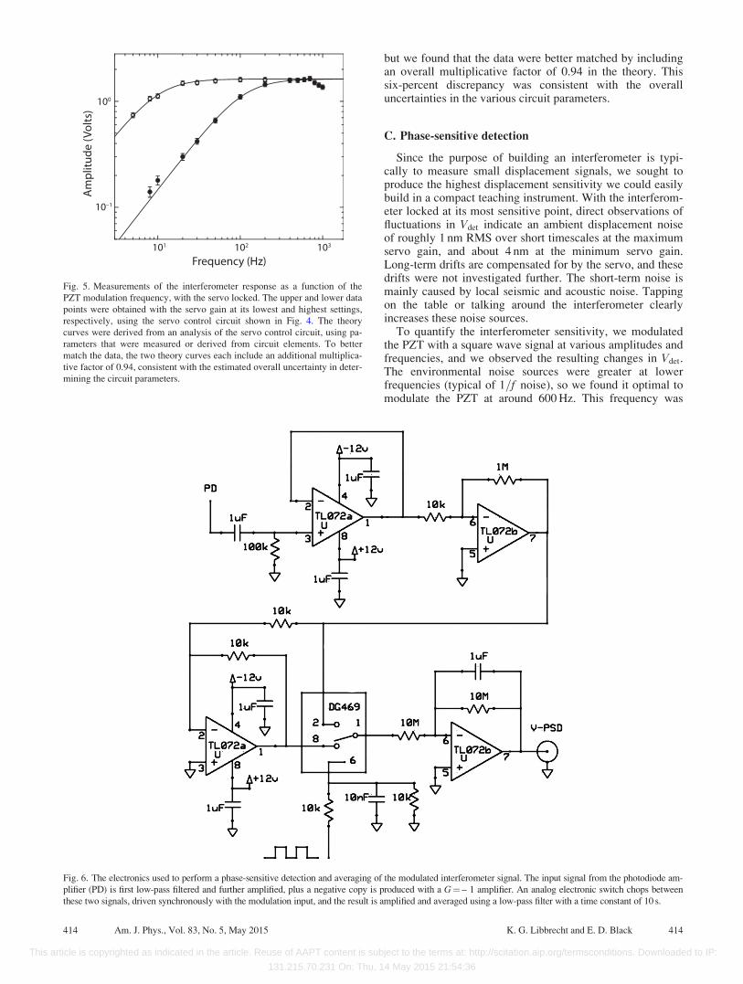
but we found that the data were better matched by includingan overall multiplicative factor of 0.94 in the theory. Thissix-percent discrepancy was consistent with the overalluncertainties in the various circuit parameters.

C. Phase-sensitive detection

Since the purpose of building an interferometer is typi-cally to measure small displacement signals, we sought toproduce the highest displacement sensitivity we could easilybuild in a compact teaching instrument. With the interferom-eter locked at its most sensitive point, direct observations offluctuations in Vdet indicate an ambient displacement noiseof roughly 1 nm RMS over short timescales at the maximumservo gain, and about 4 nm at the minimum servo gain.Long-term drifts are compensated for by the servo, and thesedrifts were not investigated further. The short-term noise ismainly caused by local seismic and acoustic noise. Tappingon the table or talking around the interferometer clearlyincreases these noise sources.

To quantify the interferometer sensitivity, we modulatedthe PZT with a square wave signal at various amplitudes andfrequencies, and we observed the resulting changes in Vdet.The environmental noise sources were greater at lowerfrequencies (typical of 1=f noise), so we found it optimal tomodulate the PZT at around 600 Hz. This frequency was

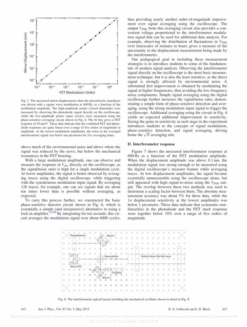
Fig. 6. The electronics used to perform a phase-sensitive detection and averaging of the modulated interferometer signal. The input signal from the photodiode am-

plifier (PD) is first low-pass filtered and further amplified, plus a negative copy is produced with a G¼ – 1 amplifier. An analog electronic switch chops between

these two signals, driven synchronously with the modulation input, and the result is amplified and averaged using a low-pass filter with a time constant of 10 s.

Frequency (Hz)

101 102 103

10–1

100

Am

plit

ud

e (

Vo

lts)

Fig. 5. Measurements of the interferometer response as a function of the

PZT modulation frequency, with the servo locked. The upper and lower data

points were obtained with the servo gain at its lowest and highest settings,

respectively, using the servo control circuit shown in Fig. 4. The theory

curves were derived from an analysis of the servo control circuit, using pa-

rameters that were measured or derived from circuit elements. To better

match the data, the two theory curves each include an additional multiplica-

tive factor of 0.94, consistent with the estimated overall uncertainty in deter-

mining the circuit parameters.

414 Am. J. Phys., Vol. 83, No. 5, May 2015 K. G. Libbrecht and E. D. Black 414

This article is copyrighted as indicated in the article. Reuse of AAPT content is subject to the terms at: http://scitation.aip.org/termsconditions. Downloaded to IP:

131.215.70.231 On: Thu, 14 May 2015 21:54:36

above much of the environmental noise and above where thesignal was reduced by the servo, but below the mechanicalresonances in the PZT housing.

With a large modulation amplitude, one can observe andmeasure the response in Vdet directly on the oscilloscope, asthe signal/noise ratio is high for a single modulation cycle.At lower amplitudes, the signal is better observed by averag-ing traces using the digital oscilloscope, while triggeringwith the synchronous modulation input signal. By averaging128 traces, for example, one can see signals that are aboutten times lower than is possible without averaging, asexpected.

To carry this process further, we constructed the basicphase-sensitive detector circuit shown in Fig. 6, which isessentially a simple (and inexpensive) alternative to using alock-in amplifier.19,20 By integrating for ten seconds, this cir-cuit averages the modulation signal over about 6000 cycles,

thus providing nearly another order-of-magnitude improve-ment over signal averaging using the oscilloscope. Theoutput VPSD from this averaging circuit also provides a con-venient voltage proportional to the interferometer modula-tion signal that can be used for additional data analysis. Forexample, observing the distribution of fluctuations in VPSD

over timescales of minutes to hours gives a measure of theuncertainty in the displacement measurement being made bythe interferometer.

Our pedagogical goal in including these measurementstrategies is to introduce students to some of the fundamen-tals of modern signal analysis. Observing the interferometersignal directly on the oscilloscope is the most basic measure-ment technique, but it is also the least sensitive, as the directsignal is strongly affected by environmental noise. Asubstantial first improvement is obtained by modulating thesignal at higher frequencies, thus avoiding the low-frequencynoise components. Simple signal averaging using the digitaloscilloscope further increases the signal/noise ratio, demon-strating a simple form of phase-sensitive detection and aver-aging, using the strong modulation input signal to trigger theoscilloscope. Additional averaging using the circuit in Fig. 4yields an expected additional improvement in sensitivity.Seeing the gains in sensitivity at each stage in the experimentintroduces students to the concepts of signal modulation,phase-sensitive detection, and signal averaging, drivinghome the

ffiffiffiffiNp

averaging rule.

D. Interferometer response

Figure 7 shows the measured interferometer response at600 Hz as a function of the PZT modulation amplitude.When the displacement amplitude was above 0.1 nm, themodulation signal was strong enough to be measured usingthe digital oscilloscope’s measure feature while averagingtraces. At low displacement amplitudes, the signal becameessentially unmeasurable using the oscilloscope alone, butstill appeared with high signal-to-noise using the VPSD out-put. The overlap between these two methods was used todetermine a scaling factor between them. The absolute mea-surement accuracy was about 5% for these data, while the1r displacement sensitivity at the lowest amplitudes wasbelow 1 picometer. These data indicate that systematic non-linearities in the photodiode and the PZT stack responsewere together below 10% over a range of five orders ofmagnitude.

10–410–5 10–3 10–2 10–1 100

PZT Modulation (Volts)

Mir

ror

Dis

pla

cem

en

t (n

m)

10–3

10–2

10–1

101

100

102

Fig. 7. The measured mirror displacement when the piezoelectric transducer

was driven with a square wave modulation at 600 Hz, as a function of the

modulation amplitude. The high-amplitude points (closed diamonds) were

measured by observing the photodiode signal directly on the oscilloscope,

while the low-amplitude points (open circles) were measured using the

phase-sensitive averaging circuit shown in Fig. 6. The fit line gives a PZT

response of 45 nm/V. These data indicate that the combined PZT and photo-

diode responses are quite linear over a range of five orders of magnitude in

amplitude. At the lowest modulation amplitudes, the noise in the averaged

interferometer signal was below one picometer for 10-s averaging times.

Mirror/PZT

Mirror 1

Beamsplitter

Photodetector

Helium-Neon (He-Ne) Laser

Mirror 2

Oscillator

Fig. 8. The interferometer optical layout including the mechanical oscillator shown in detail in Fig. 9.

415 Am. J. Phys., Vol. 83, No. 5, May 2015 K. G. Libbrecht and E. D. Black 415

This article is copyrighted as indicated in the article. Reuse of AAPT content is subject to the terms at: http://scitation.aip.org/termsconditions. Downloaded to IP:

131.215.70.231 On: Thu, 14 May 2015 21:54:36

III. MEASURING A SIMPLE HARMONIC

OSCILLATOR

Once students have constructed, aligned, and character-ized the interferometer, they can then use it to observe thenanoscale motions of a simple harmonic oscillator.21 Theoptical layout for this second stage of the experiment isshown in Fig. 8, and the mechanical construction of theoscillator is shown in Fig. 9. Wiring for the coil runs througha vertical hole in the aluminum plate (below the coil but notshown in Fig. 9) and then through one of the holes in thebreadboard to the electronics chassis below. For this reasonthe oscillator position on the breadboard cannot be changed,but it does not interfere with the basic interferometer layoutshown in Fig. 1.

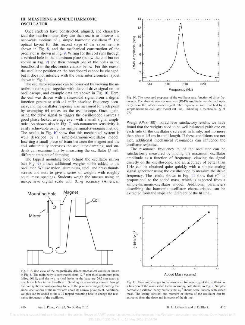
The oscillator response can be observed by viewing the in-terferometer signal together with the coil drive signal on theoscilloscope, and example data are shown in Fig. 10. Here,the coil was driven with a sinusoidal signal from a digitalfunction generator with <1 mHz absolute frequency accu-racy, and the oscillator response was measured for each pointby averaging 64 traces on the oscilloscope. Once again,using the drive signal to trigger the oscilloscope ensures agood phase-locked average even with a small signal ampli-tude. As shown also in Fig. 7, sub-nanometer sensitivity iseasily achievable using this simple signal-averaging method.The results in Fig. 10 show that this mechanical system iswell described by a simple-harmonic-oscillator model.Inserting a small piece of foam between the magnet and thecoil substantially increases the oscillator damping, and stu-dents can examine this by measuring the oscillator Q withdifferent amounts of damping.

The tapped mounting hole behind the oscillator mirror(see Fig. 9) allows additional weights to be added to theoscillator. We use nylon, aluminium, steel, and brass thumb-screws and nuts to give a series of weights with roughlyequal mass spacings. Students weigh the masses using aninexpensive digital scale with 0.1-g accuracy (American

Weigh AWS-100). To achieve satisfactory results, we havefound that the weights need to be well balanced (with one oneach side of the oscillator), screwed in firmly, and no morethan about 1.5 cm in total length. If these conditions are notmet, additional mechanical resonances can influence theoscillator response.

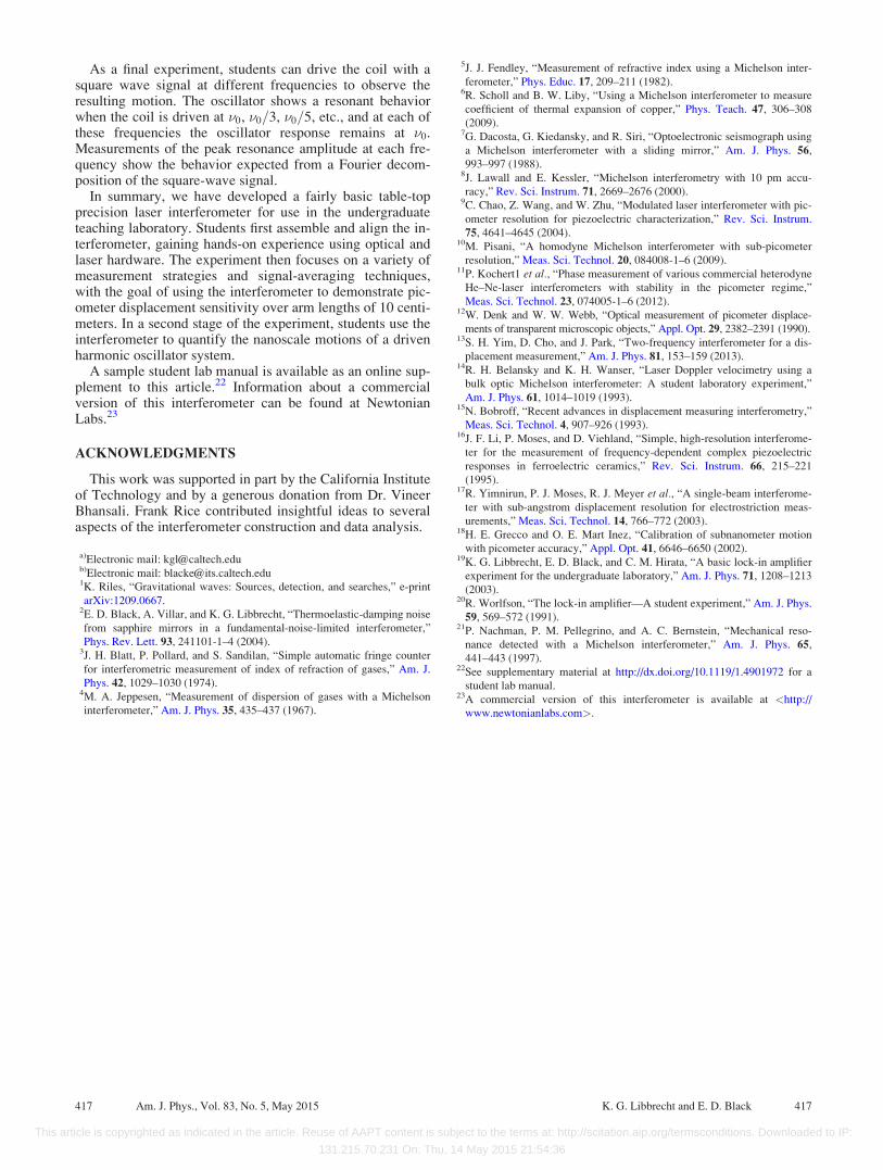
The resonance frequency �0 of the oscillator can besatisfactorily measured by finding the maximum oscillatoramplitude as a function of frequency, viewing the signaldirectly on the oscilloscope, and an accuracy of better than1 Hz can be obtained quite quickly with a simple analogsignal generator using the oscilloscope to measure the drivefrequency. The results shown in Fig. 11 show that ��2

0 isproportional to the added mass, which is expected from asimple-harmonic-oscillator model. Additional parametersdescribing the harmonic oscillator characteristics can beextracted from the slope and intercept of the fit line.

Fig. 10. The measured response of the oscillator as a function of drive fre-

quency. The absolute root-mean-square (RMS) amplitude was derived opti-

cally from the interferometer signal. The response is well matched by a

simple-harmonic-oscillator model (fit line), indicating a mechanical Q of

970.

Fig. 11. Measured changes in the resonance frequency �0 of the oscillator as

a function of the mass added to the mounting hole shown in Fig. 9. Simple-

harmonic-oscillator theory predicts that ��20 should scale linearly with added

mass. The spring constant and moment of inertia of the oscillator can be

extracted from the slope and intercept of the fit line.

Mirror

Magnet

Coil

Mounting Hole

Fig. 9. A side view of the magnetically driven mechanical oscillator shown

in Fig. 8. The main body is constructed from 12.7-mm-thick aluminum plate

(alloy 6061), and the two vertical holes in the base are 76.2 mm apart to

match the holes in the breadboard. Sending an alternating current through

the coil applies a corresponding force to the permanent magnet, driving tor-

sional oscillations of the mirror arm about its narrow pivot point. Additional

weights can be added to the 8-32 tapped mounting hole to change the reso-

nance frequency of the oscillator.

416 Am. J. Phys., Vol. 83, No. 5, May 2015 K. G. Libbrecht and E. D. Black 416

This article is copyrighted as indicated in the article. Reuse of AAPT content is subject to the terms at: http://scitation.aip.org/termsconditions. Downloaded to IP:

131.215.70.231 On: Thu, 14 May 2015 21:54:36

As a final experiment, students can drive the coil with asquare wave signal at different frequencies to observe theresulting motion. The oscillator shows a resonant behaviorwhen the coil is driven at �0, �0=3, �0=5, etc., and at each ofthese frequencies the oscillator response remains at �0.Measurements of the peak resonance amplitude at each fre-quency show the behavior expected from a Fourier decom-position of the square-wave signal.

In summary, we have developed a fairly basic table-topprecision laser interferometer for use in the undergraduateteaching laboratory. Students first assemble and align the in-terferometer, gaining hands-on experience using optical andlaser hardware. The experiment then focuses on a variety ofmeasurement strategies and signal-averaging techniques,with the goal of using the interferometer to demonstrate pic-ometer displacement sensitivity over arm lengths of 10 centi-meters. In a second stage of the experiment, students use theinterferometer to quantify the nanoscale motions of a drivenharmonic oscillator system.

A sample student lab manual is available as an online sup-plement to this article.22 Information about a commercialversion of this interferometer can be found at NewtonianLabs.23

ACKNOWLEDGMENTS

This work was supported in part by the California Instituteof Technology and by a generous donation from Dr. VineerBhansali. Frank Rice contributed insightful ideas to severalaspects of the interferometer construction and data analysis.

a)Electronic mail: kgl@caltech.edub)Electronic mail: blacke@its.caltech.edu1K. Riles, “Gravitational waves: Sources, detection, and searches,” e-print

arXiv:1209.0667.2E. D. Black, A. Villar, and K. G. Libbrecht, “Thermoelastic-damping noise

from sapphire mirrors in a fundamental-noise-limited interferometer,”

Phys. Rev. Lett. 93, 241101-1–4 (2004).3J. H. Blatt, P. Pollard, and S. Sandilan, “Simple automatic fringe counter

for interferometric measurement of index of refraction of gases,” Am. J.

Phys. 42, 1029–1030 (1974).4M. A. Jeppesen, “Measurement of dispersion of gases with a Michelson

interferometer,” Am. J. Phys. 35, 435–437 (1967).

5J. J. Fendley, “Measurement of refractive index using a Michelson inter-

ferometer,” Phys. Educ. 17, 209–211 (1982).6R. Scholl and B. W. Liby, “Using a Michelson interferometer to measure

coefficient of thermal expansion of copper,” Phys. Teach. 47, 306–308

(2009).7G. Dacosta, G. Kiedansky, and R. Siri, “Optoelectronic seismograph using

a Michelson interferometer with a sliding mirror,” Am. J. Phys. 56,

993–997 (1988).8J. Lawall and E. Kessler, “Michelson interferometry with 10 pm accu-

racy,” Rev. Sci. Instrum. 71, 2669–2676 (2000).9C. Chao, Z. Wang, and W. Zhu, “Modulated laser interferometer with pic-

ometer resolution for piezoelectric characterization,” Rev. Sci. Instrum.

75, 4641–4645 (2004).10M. Pisani, “A homodyne Michelson interferometer with sub-picometer

resolution,” Meas. Sci. Technol. 20, 084008-1–6 (2009).11P. Kochert1 et al., “Phase measurement of various commercial heterodyne

He–Ne-laser interferometers with stability in the picometer regime,”

Meas. Sci. Technol. 23, 074005-1–6 (2012).12W. Denk and W. W. Webb, “Optical measurement of picometer displace-

ments of transparent microscopic objects,” Appl. Opt. 29, 2382–2391 (1990).13S. H. Yim, D. Cho, and J. Park, “Two-frequency interferometer for a dis-

placement measurement,” Am. J. Phys. 81, 153–159 (2013).14R. H. Belansky and K. H. Wanser, “Laser Doppler velocimetry using a

bulk optic Michelson interferometer: A student laboratory experiment,”

Am. J. Phys. 61, 1014–1019 (1993).15N. Bobroff, “Recent advances in displacement measuring interferometry,”

Meas. Sci. Technol. 4, 907–926 (1993).16J. F. Li, P. Moses, and D. Viehland, “Simple, high-resolution interferome-

ter for the measurement of frequency-dependent complex piezoelectric

responses in ferroelectric ceramics,” Rev. Sci. Instrum. 66, 215–221

(1995).17R. Yimnirun, P. J. Moses, R. J. Meyer et al., “A single-beam interferome-

ter with sub-angstrom displacement resolution for electrostriction meas-

urements,” Meas. Sci. Technol. 14, 766–772 (2003).18H. E. Grecco and O. E. Mart Inez, “Calibration of subnanometer motion

with picometer accuracy,” Appl. Opt. 41, 6646–6650 (2002).19K. G. Libbrecht, E. D. Black, and C. M. Hirata, “A basic lock-in amplifier

experiment for the undergraduate laboratory,” Am. J. Phys. 71, 1208–1213

(2003).20R. Worlfson, “The lock-in amplifier—A student experiment,” Am. J. Phys.

59, 569–572 (1991).21P. Nachman, P. M. Pellegrino, and A. C. Bernstein, “Mechanical reso-

nance detected with a Michelson interferometer,” Am. J. Phys. 65,

441–443 (1997).22See supplementary material at http://dx.doi.org/10.1119/1.4901972 for a

student lab manual.23A commercial version of this interferometer is available at <http://

www.newtonianlabs.com>.

417 Am. J. Phys., Vol. 83, No. 5, May 2015 K. G. Libbrecht and E. D. Black 417

This article is copyrighted as indicated in the article. Reuse of AAPT content is subject to the terms at: http://scitation.aip.org/termsconditions. Downloaded to IP:

131.215.70.231 On: Thu, 14 May 2015 21:54:36