A basic geometric morphometric analysisg562/PBDB2013/Day 2B - Geometric Morphometric… · A basic...
30
Department of Geological Sciences | Indiana University (c) 2012, P. David Polly G562 Geometric Morphometrics Step by step in R A basic geometric morphometric analysis
Transcript of A basic geometric morphometric analysisg562/PBDB2013/Day 2B - Geometric Morphometric… · A basic...

Department of Geological Sciences | Indiana University (c) 2012, P. David Polly
G562 Geometric Morphometrics
Step by step in R
A basic geometric morphometric analysis
Department of Geological Sciences | Indiana University (c) 2012, P. David Polly
G562 Geometric Morphometrics
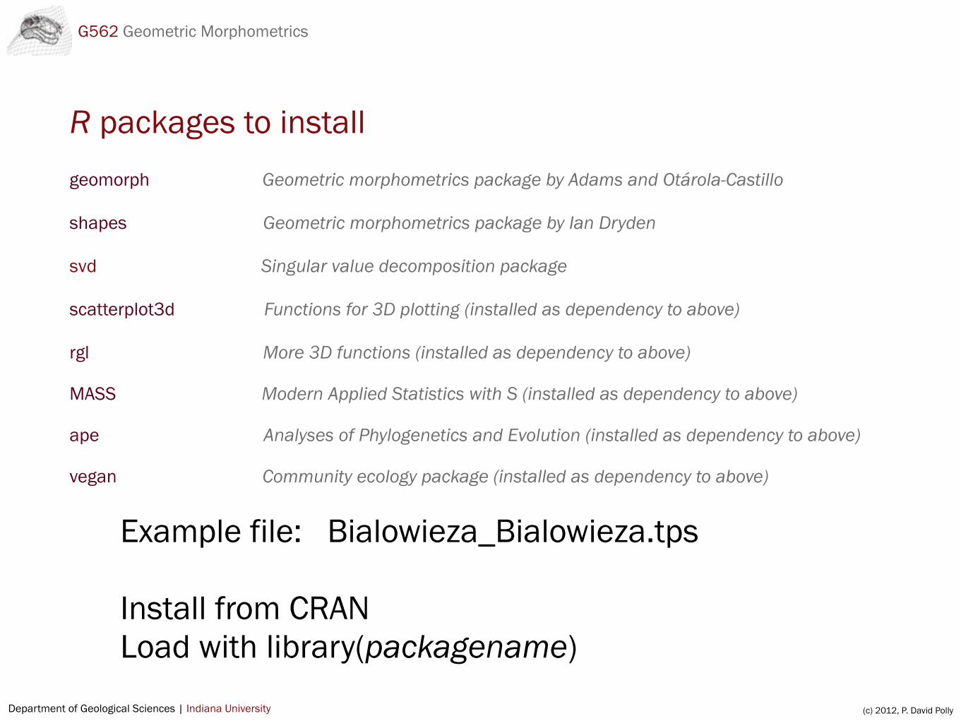
R packages to installgeomorph Geometric morphometrics package by Adams and Otárola-Castillo
shapes Geometric morphometrics package by Ian Dryden
svd Singular value decomposition package
scatterplot3d Functions for 3D plotting (installed as dependency to above)
rgl More 3D functions (installed as dependency to above)
MASS Modern Applied Statistics with S (installed as dependency to above)
ape Analyses of Phylogenetics and Evolution (installed as dependency to above)
vegan Community ecology package (installed as dependency to above)
Example file: Bialowieza_Bialowieza.tps
Install from CRANLoad with library(packagename)

Department of Geological Sciences | Indiana University (c) 2012, P. David Polly
G562 Geometric Morphometrics
Study design
Data collection
Data standardization
Analysis
Results interpretation
General Procedure
Department of Geological Sciences | Indiana University (c) 2012, P. David Polly
G562 Geometric Morphometrics
Steps in a geometric morphometric analysis
1. Obtain landmark coordinates.
2. Standarization: Procrustes superimposition of the landmarks.removes size, translation, and rotation (also project to tangent space for further statistical analysis).
3. Standardization: Create shape variables (variables that retain information about shape, but are uncorrelated with one another and have appropriate degrees of freedom)PCA scores are one kind of shape variable that satisfy these requirements
4. Analysis: Conduct further analyses on the shape variablesType of analysis required depends on questions being addressedRegression, ANOVA, path analysis, tree-building, etc.

Department of Geological Sciences | Indiana University (c) 2012, P. David Polly
G562 Geometric Morphometrics
Choosing landmarks
1. landmarks should sample the aspects of the shape that are of interest
2. enough landmarks should be used to adequately sample the shape
3. don’t oversample (NB: each landmark adds weight to the analysis. Multiple landmarks on one area will increase weight of that area.)
4. landmarks should be repeatable (same point on every specimen, placed with as little error as possible)
1. type 1 = location of the point defined by obvious biologically homologous structures (eg. intersection of three bones)
2. type 2 = location of the point defined by obvious geometry (eg., point of greatest curvature)
3. type 3 = location of point defined with reference to another point (eg., point ventral to last tooth)
5. landmarks must be placed in the same order on all specimens

Department of Geological Sciences | Indiana University (c) 2012, P. David Polly
G562 Geometric Morphometrics
Obtaining landmark coordinates
From a file
lands <- readland.tps(file.choose()) [imports from TPS format file]
lands <- readland.nts(file.choose()) [imports from NTS format file]
From an image
digitize2d(filename, landmarks, scale) [opens jpg file and collects lands]
Note: digitize2d may need debugging. Saves coordinates to file in working directory in NTS format.
readmulti.nts(filenames)

Department of Geological Sciences | Indiana University(c) 2012, P. David Polly
digitize2d()Erik Otarola-Castillo has sent a fix. Do the following and the function will work:
1. Set the working directory to where your images are stored.2. Define the function picscale() as follows
picscale <- function(scale){ digscale<-NULL digscale<-locator(2,type="o",lwd=2,col="red",lty="11") sqrt(sum(diff(digscale$x)^2 + diff(digscale$y)^2))*scale}
To collection landmarks in digitize2d:
1. If you have a scale bar in the images
1.1. enter the length of the scale bar as argument (e.g., 10 if the scale bar is 10 mm)1.2. when digitize2d starts, click on both ends of the scale bar, then click on your
landmarks in the proper order1.3. coordinates and centroid sizes will be scaled in the units of your scale bar (e.g., mm)
2. If you don’t have a scale bar:
2.1. enter 1 as the scale argument 2.2. when digitize2d starts, click in two arbitrary but different places on the image, then
click on your landmarks in the proper order2.3. coordinates will have no real units and centroid size will be meaningless

Department of Geological Sciences | Indiana University (c) 2012, P. David Polly
G562 Geometric Morphometrics
Automate the digitizing and loading of files
Digitize.My.Files <- edit()
function(path, lands, scale) {setwd(path)myFiles <- dir(pattern="[jJ][pP][gG]")for( i in 1:length( myFiles ) ) { dig2d(myFiles[i],lands, scale)}myFiles <- dir(pattern="[nN][tT][sS]")return(readmulti.nts(myFiles))}
mylands <- Digitize.My.Files(“/Users/pdavidpolly/ShrewsAndMarmots”, 10, 10)

Department of Geological Sciences | Indiana University (c) 2012, P. David Polly
G562 Geometric Morphometrics
Cryptic error? Error in .External2(C_edit, name, file, title, editor) : unexpected input occurred on line 3 use a command like x <- edit() to recover
May be caused by smart quotes if you copied and pasted script from Word or other text editor

Department of Geological Sciences | Indiana University (c) 2012, P. David Polly
G562 Geometric Morphometrics
Performing Procrustes analysis and obtaining shape variables
Also known as Generalized Procrustes Analysis (GPA)
> gpa.lands <- gpagen(lands)
results of gpagen() include:
1. a plot of the superimposed specimens and their consensus (mean) shape
2. superimposed coordinates ($coords)
3. shape variables as principal components scores ($pc.scores)
Department of Geological Sciences | Indiana University (c) 2012, P. David Polly
G562 Geometric Morphometrics
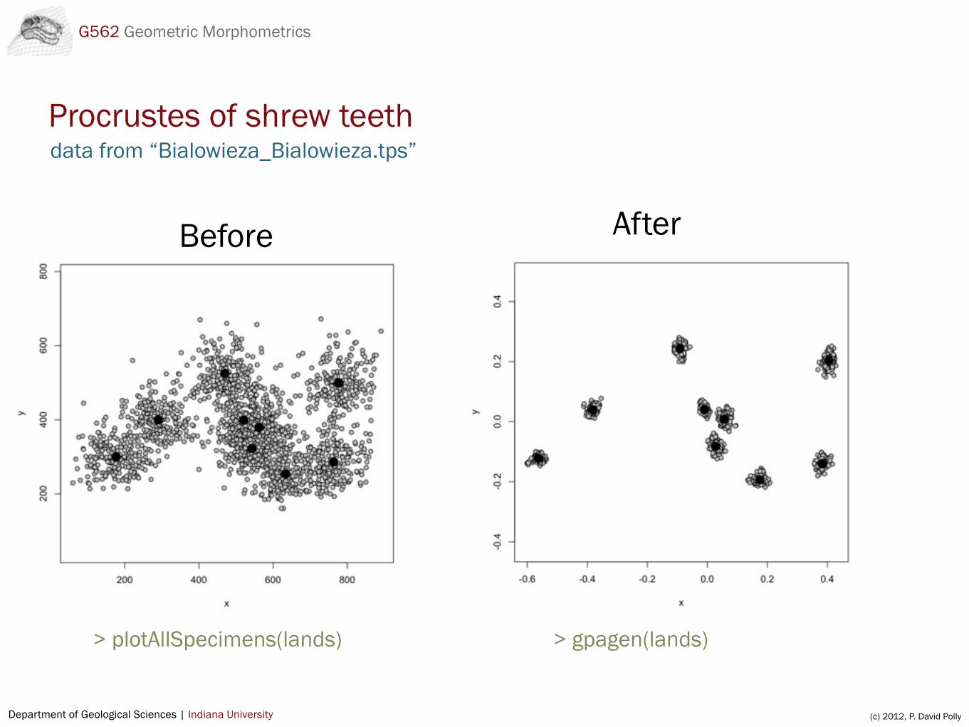
Procrustes of shrew teeth
Before After
> plotAllSpecimens(lands) > gpagen(lands)
data from “Bialowieza_Bialowieza.tps”

Department of Geological Sciences | Indiana University (c) 2012, P. David Polly
G562 Geometric Morphometrics
Details of gpagen()• proc <- gpagen(
• This function does a generalized Procrustes analysis, superimposition of multiple specimens about their mean (Gower, 1975; Rohlf and Slice, 1990)
• Returns a plot of superimposed coordinates
• Returns the superimposed coordinates and their centroid sizes in dataframe format:
• $coords = the x,y(,z) Procrustes coordinates after superimposition
• $Csize = the centroid size of the specimens
To plot the Procrustes coordinates yourself:
for(i in 1:dim(proc$coords)[3]) points(proc$coords[,,i])
plotAllSpecimens(proc$coords)
Department of Geological Sciences | Indiana University (c) 2012, P. David Polly
G562 Geometric Morphometrics
Creating a principal components plot
> pca.lands <- plotTangentSpace(proc$coords, label=TRUE)
results of plotTangentSpace() include:
1. a plot of the specimens in principal components space and two thin plate spline grids showing the shapes associated with the positive and negative ends of the horizontal axis (default = PC1 x PC2 set axes using the args axis1 and axis2)
2. summary of variance associated with each PC axis ($pc.summary)
3. shape variables as principal components scores ($pc.scores)

Department of Geological Sciences | Indiana University (c) 2012, P. David Polly
G562 Geometric Morphometrics
Principal component plot of shrew teeth
Thin plate spline grid of shape at positive
end of 1st axis
Thin plate spline grid of shape at negative end of
1st axis
PC 1
PC 2

Department of Geological Sciences | Indiana University (c) 2012, P. David Polly
G562 Geometric Morphometrics
Variance explained by PC axespca.lands$pc.summary

Department of Geological Sciences | Indiana University (c) 2012, P. David Polly
G562 Geometric Morphometrics
Important concept: variance of a data set
Variance = variability = shape variation
PC scores preserve the shape variation in the original data
Variance = average squared distance from the mean
Variance in Procrustes coordinates = Variance in PC scores
> sum(pca.lands$pc.summary$sdev^2)
> sum(apply(pca.lands$pc.scores, 2, var))
> sum(apply(proc$coords,c(1,2),var))
Department of Geological Sciences | Indiana University (c) 2012, P. David Polly
G562 Geometric Morphometrics
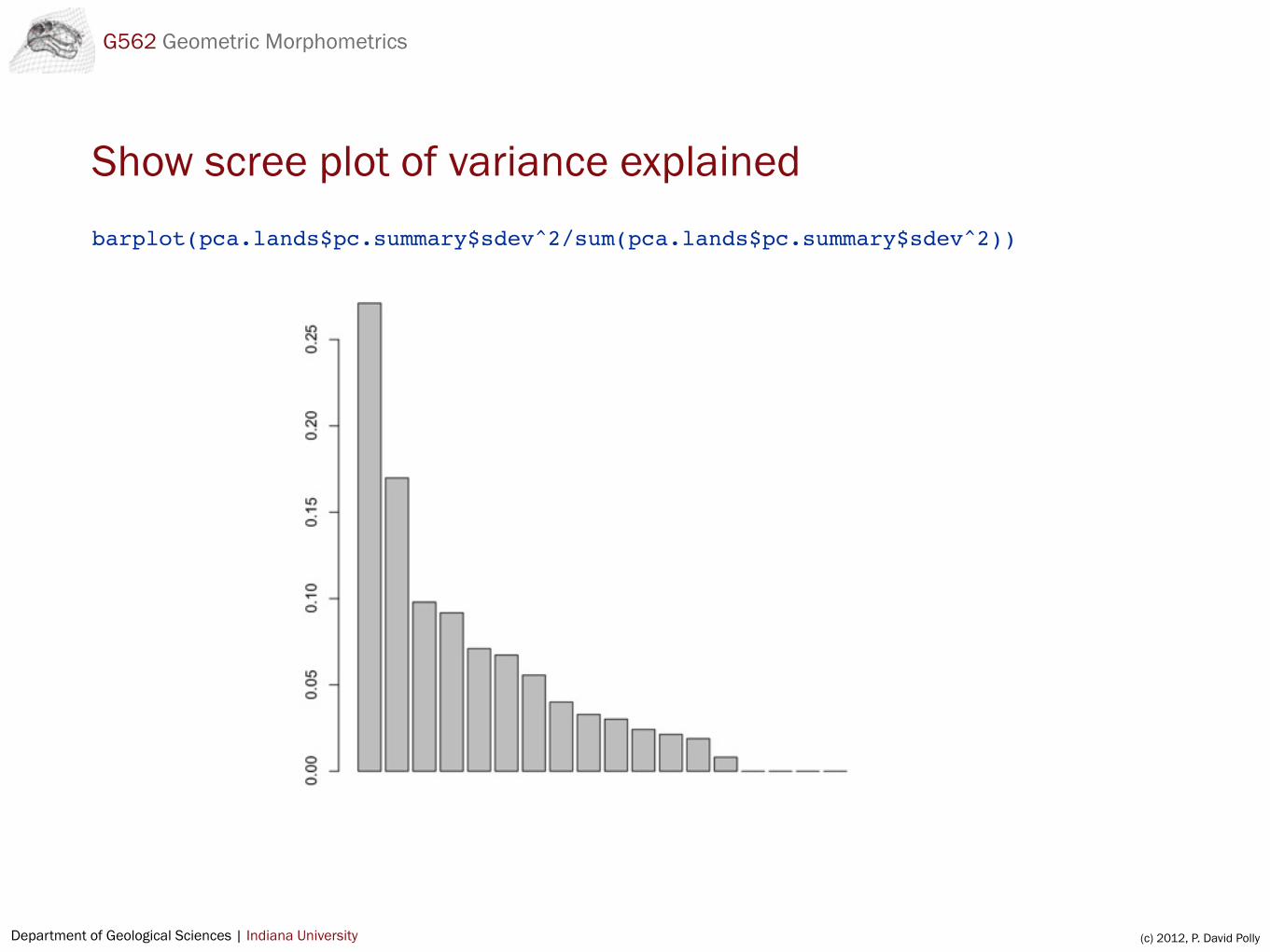
Show scree plot of variance explainedbarplot(pca.lands$pc.summary$sdev^2/sum(pca.lands$pc.summary$sdev^2))

Department of Geological Sciences | Indiana University (c) 2012, P. David Polly
G562 Geometric Morphometrics
Create your own customized plot> plot(pca.lands$pc.scores[,1:2],pch=15,xlab="PC1",ylab="PC2")
> text(pca.lands$pc.scores[,1:2],rownames(pca.lands$pc.scores[,1:2]),pos=4,cex=.5)

Department of Geological Sciences | Indiana University (c) 2012, P. David Polly
G562 Geometric Morphometrics
Create 3D scatterplot> library(scatterplot3d)
> scatterplot3d(pca.lands$pc.scores[,1:3])

Department of Geological Sciences | Indiana University (c) 2012, P. David Polly
G562 Geometric Morphometrics
Terminology: shape
Shape = a set of landmarks
Sometimes “shape” specifically refers to the landmark configurations without respect to size and “form” refers to the configurations including size

Department of Geological Sciences | Indiana University (c) 2012, P. David Polly
G562 Geometric Morphometrics
Terminology: Consensus shape
Consensus shape = mean shape
Average x,y coordinate of each landmark after Procrustes alignment
To calculate
> consensus <- apply(proc$coords, c(1,2), mean)
> plot(consensus,asp=1, type="n")
> for(i in 1:length(proc$coords[,,3])) points(proc$coords[,,i])
> points(consensus, col=”Red”, cex=2, pch=20)

Department of Geological Sciences | Indiana University (c) 2012, P. David Polly
G562 Geometric Morphometrics
Terminology: centroid
The mean (center) of a shape (or of a landmark). Average x,y of all coordinates across all landmarks. (for individual landmark, the centroid is the consensus point for that landmark).
To calculate:
> centroid <- apply(proc$coords,2,mean)

Department of Geological Sciences | Indiana University (c) 2012, P. David Polly
G562 Geometric Morphometrics
-150 -100 -50 0 50 100 150
-150
-100
-50
050
100
150
PC1
PC2 Shrew
Squirrel
Shrew
Mouse
Squirrel
Position of consensus shape
[40.2,-22.2]
Scores on PC1 and PC2 for fourth specimen
[-67.3,0.77]
Scores on PC1 and PC2 for first specimen
Finding your way around shape space
Department of Geological Sciences | Indiana University (c) 2012, P. David Polly
G562 Geometric Morphometrics
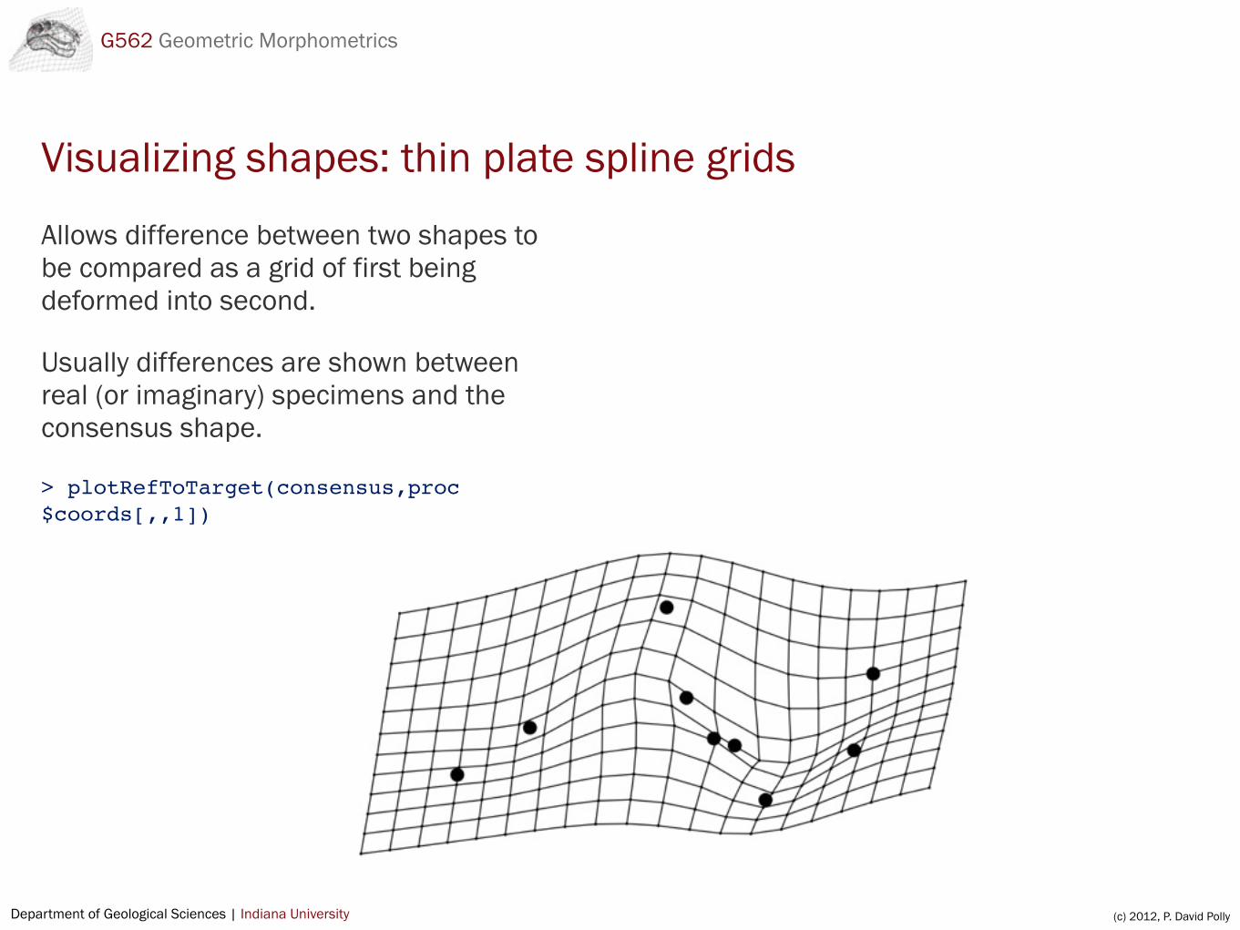
Visualizing shapes: thin plate spline grids
Allows difference between two shapes to be compared as a grid of first being deformed into second.
Usually differences are shown between real (or imaginary) specimens and the consensus shape.
> plotRefToTarget(consensus,proc$coords[,,1])

Department of Geological Sciences | Indiana University (c) 2012, P. David Polly
G562 Geometric Morphometrics
Principles of shape space
1. PCA space = shape space
2. Every point in shape space corresponds to configuration of landmarks
3. By definition, the consensus (mean shape) lies at the origin (0,0) of the shape space
4. PC scores are the coordinates of the PCA plot (they are the “addresses” of the points in the shape space)

Department of Geological Sciences | Indiana University (c) 2012, P. David Polly
G562 Geometric Morphometrics
Landmark Space (specimen space)
Two (or three) dimensional space (x, y, z)
Numbers associated with space are the landmark coordinates
Many points per specimen
Shape Space (PCA space)
Multidimensional space (nearly as many dimensions as there are landmarks x
coordinates)
Numbers are scores (addresses in PC space)
One point per specimen

Department of Geological Sciences | Indiana University (c) 2012, P. David Polly
G562 Geometric Morphometrics
Basic steps of shape analysis in R
Capture imagesdigital camera, etc.
Collect coordinatesdigitize2d(filename)
Read coordinate files in NTS formatreadmulti.nts(filenames)
Superimpose landmarks and do PCAgpagen(lands)
View PCA resultsplotTangentSpace($coords)
Look at shape differencesplotRefToTarget(shape1, shape2)
Department of Geological Sciences | Indiana University (c) 2012, P. David Polly
G562 Geometric Morphometrics
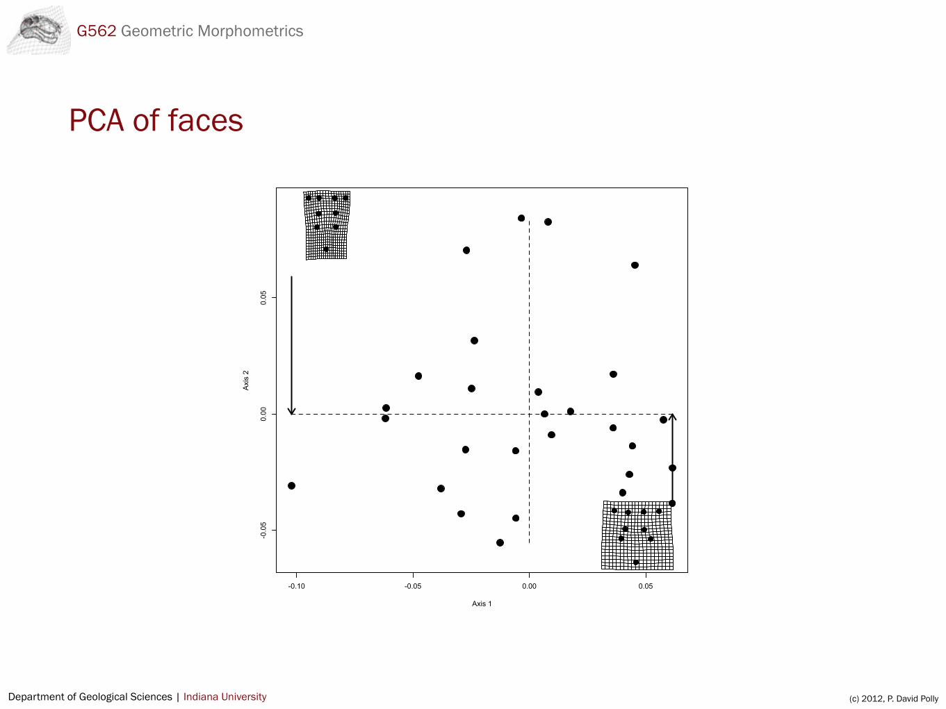
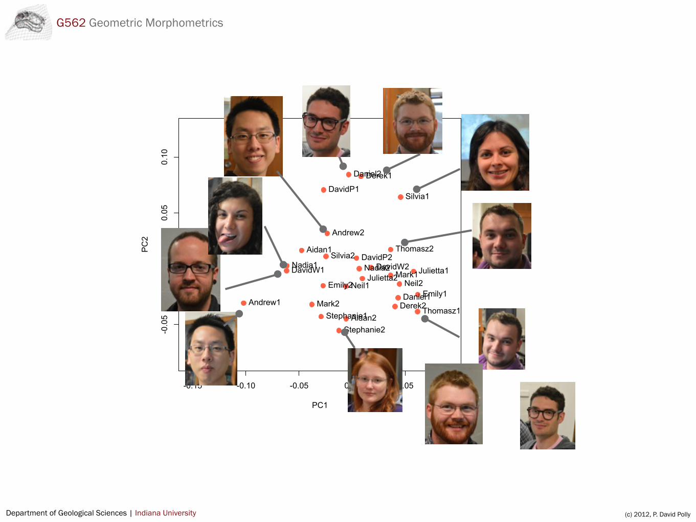
PCA of faces
-0.10 -0.05 0.00 0.05
-0.05
0.00
0.05
Axis 1
Axi
s 2

Department of Geological Sciences | Indiana University (c) 2012, P. David Polly
G562 Geometric Morphometrics
-0.15 -0.10 -0.05 0.00 0.05 0.10
-0.05
0.00
0.05
0.10
PC1
PC2
Andrew1
Nadia1
Thomasz1
Julietta1Mark1DavidW1
Daniel1
Derek1
Emily1
Aidan1
Stephanie1
Neil1
Silvia1DavidP1
Andrew2
Nadia2
Thomasz2
Julietta2
Mark2
DavidW2
Daniel2
Derek2
Emily2
Aidan2Stephanie2
Neil2
Silvia2 DavidP2