൮ “Modeling surface appearance from a single …‘£悦.pdfModeling Surface Appearance from a...
53
Xiao Li 1,2 Yue Dong 2 Pieter Peers 3 Xin Tong 2 1 University of Science and Technology of China 2 Microsoft Research, Beijing 3 College of William & Mary Modeling Surface Appearance from a Single Photograph using Self-Augmented Convolutional Neural Networks
Transcript of ൮ “Modeling surface appearance from a single …‘£悦.pdfModeling Surface Appearance from a...

Xiao Li1,2 Yue Dong2 Pieter Peers3 Xin Tong2
1 University of Science and Technology of China2 Microsoft Research, Beijing3 College of William & Mary
Modeling Surface Appearance from a Single Photograph usingSelf-Augmented Convolutional Neural Networks
演示者
演示文稿备注
Good afternoon. My name is Xiao Li from University of Science and Technology of China, and I will talk about our latest work on “Modeling surface appearance from a single photograph using self-augmented convolutional neural networks”.

Appearance Modeling from Single Image
Modeling Process
Input Image
Albedo Map Bump Map
Specular
演示者
演示文稿备注
Appearance modeling from a single image plays a very important role in computer graphics. Given a reference photo, experienced artists is able to generate texture maps, bump normal maps, and specular parameters.

Artists’ Solution
Professional software
Experienced artist
Input Image
Albedo Map Bump Map
Specular
Manual Interactions
演示者
演示文稿备注
However, generate appearance from single image is a time-consuming and tedious work. Usually, artist need to use professional software like MAYA or Photoshop, and process the image with a lot of manual interactions.

Our Goal
End to End System
Non-expert Users
Input Image
Albedo Map Bump Map
Specular
Automatic Process
演示者
演示文稿备注
So, wouldn’t it be great that we design a method that could automatically do this work? Precisely, our goal is to build a end-to-end system that given a single photograph input under uncontrolled lighting, automatically predicts plausible appearance data from it. With such system, Non-expert Users can easily generate appearance from a single texture photograph from internet and texturing their own 3D objects; it could also simplifiy artists’ process by prevent them from a lot of manual works.

Related WorkSingle image appearance modeling
• Active illumination / Known lighting– [Wang 2016]; [Xu 2016]
• Stationary / Stochastic Textures– [Wang 2011]; [Aittala 2016]
• Diffuse / homogeneous BRDF– [Barron 2015]; [Shi 2017]
• Manual interaction– [Dong 2011]
[Dong 2011]
[Aittala 2016]
演示者
演示文稿备注
For single image appearance modeling, there are some related works before and we list them here. (click) Generally, previous methods either rely on active illumination or assume that lighting is known; Some works relax lighting condition and solve for limited range of BRDF, for example, (click)focus on stationary or stochastic textures; (click)homogeneous or diffuse-only material. (click)Finally, there are also works that depends on user interactions. Still, non of those methods could automatically modeling appearance from a single photograph under uncontrolled lighting conditions.
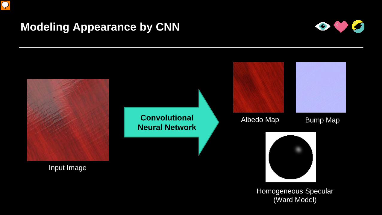
Modeling Appearance by CNN
Convolutional Neural Network
Input Image
Albedo Map Bump Map
Homogeneous Specular(Ward Model)
演示者
演示文稿备注
Artist, as we know, modeling appearance by their own knowledge; Motivated by this, we choose to using Deep Learning method to grab information from data. Given a single image input, we use conv. Nerual network to output our predictions: a spatial-variant albedo map; a spatial-variant bump normal map, and parameters representing a homogeneous specular. We choose to only output a homogeneous specular for whole image since appearance from single image is essentially a ill-posed problem, and in many cases a homogeneous specular already output plausible results.

Obtaining Labeled Data is HARD!
Input Image
Albedo Map Bump Map
Homogeneous Specular(Ward Model)
Labeled data pair
演示者
演示文稿备注
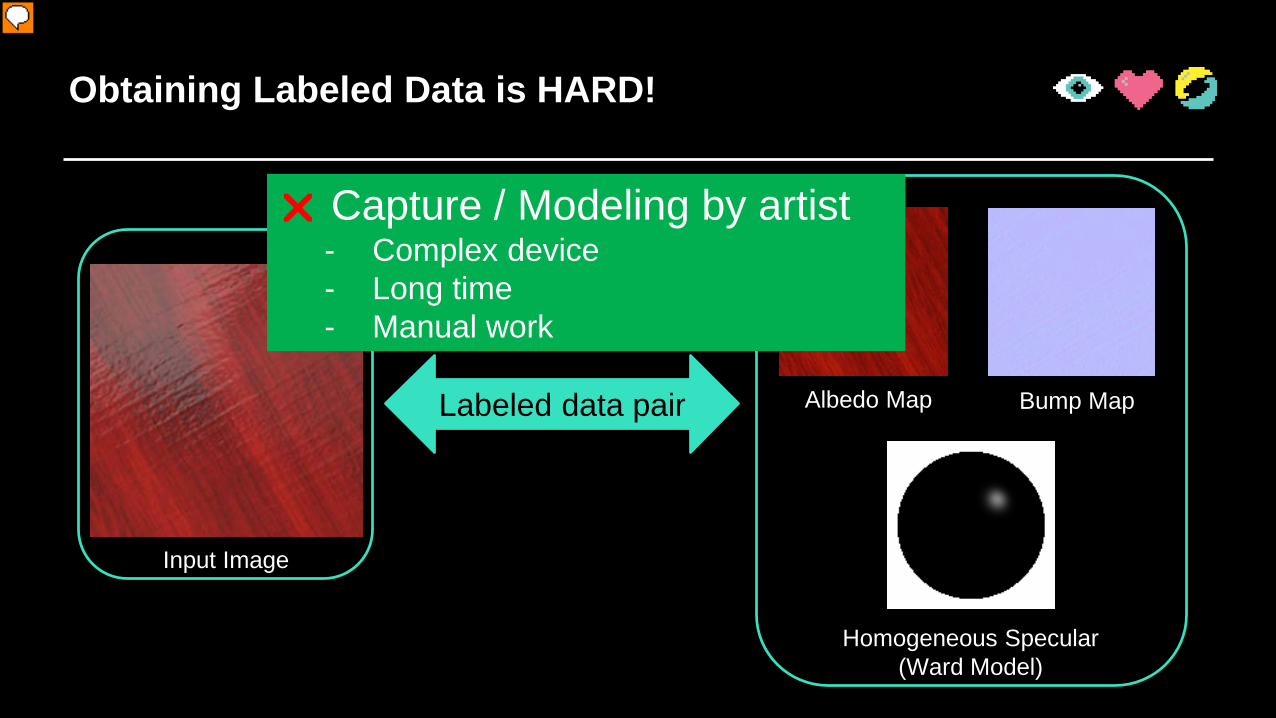
A common sense is that training a deep neural network usually needs a lot of labeled training data; In our case, labeled data means a photograph (click) and its corresponded appearance maps and values (click). However, in our scenario getting labeled data is often very hard.
Obtaining Labeled Data is HARD!
Input Image
Albedo Map Bump Map
Homogeneous Specular(Ward Model)
Labeled data pair
Capture / Modeling by artist- Complex device- Long time- Manual work
演示者
演示文稿备注
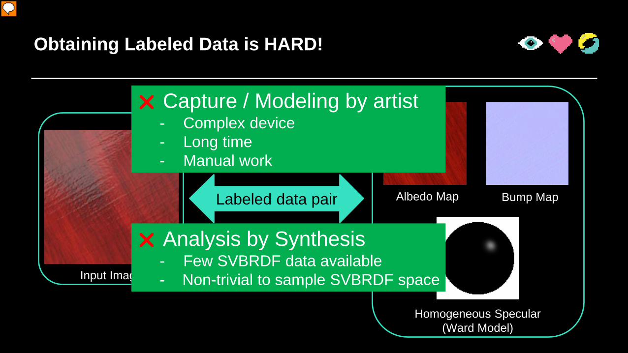
On one hand, capturing material appearance currently requires complex capturing device and very long time, or, as we have mentioned before, need a lot of manual work by artists. As a result, only few labeled examples could be collected.
Obtaining Labeled Data is HARD!
Input Image
Albedo Map Bump Map
Homogeneous Specular(Ward Model)
Labeled data pair
Capture / Modeling by artist- Complex device- Long time- Manual work
Analysis by Synthesis- Few SVBRDF data available- Non-trivial to sample SVBRDF space
演示者
演示文稿备注
Another approach is Analysis by Synthesis, which is we generate a lot of synthetic data with rendering. However, this is also very hard in our scenario. First, as mentioned before, capturing spatial variant appearance is still a very expensive process, so there are only few available dataset for rendering synthetic training data. Second, since appearance space is a very complicated high-dimensional space, it is also non-trivial to go through the space and sample from it to get enough data for synthetic rendering.

Unlabeled Image Contains Information
Highlight
演示者
演示文稿备注
So how do we overcome this problem? An observation is that, although labeled data is very hard to collect, fortunately it’s easy to obtain a lot of unlabeled images. Such image could be collected either from internet search; or from some previously released dataset, for example, the OpenSurfaces dataset. Basically, each unlabeled photograph contains information of its underline appearance. For example, the image may contain information of highlight (click);

Unlabeled Image Contains Information
Bump Effects
演示者
演示文稿备注
Or the image may contain information of its bump effects. (click) Given such large collection of unlabeled data, we then ask, is it possible to utilize this large collection of data to help our training?
Key Observation
Image AppearanceCNN
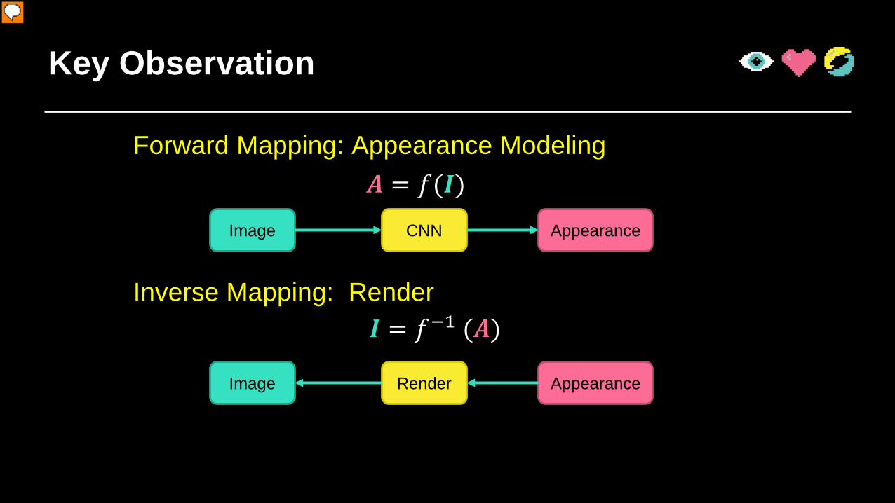
𝑨𝑨 = 𝑓𝑓(𝑰𝑰)
Image AppearanceRender
𝑰𝑰 = 𝑓𝑓−1 (𝑨𝑨)Inverse Mapping: Render
Forward Mapping: Appearance Modeling
演示者
演示文稿备注
So eventually the answer is “yes”. The key observation here is that, for this single image appearace modeling problem we want to solve (click), we actually have a well-defined inverse mapping, which is, rendering. (click) Our task is getting the appearance from a image, but given the appearance, we can render out one image which is our input. (click)
Key Observation
Image AppearanceCNN
𝐴𝐴 = 𝑓𝑓(𝐼𝐼)
Image AppearanceRender
𝐼𝐼 = 𝑓𝑓−1 (𝐴𝐴)
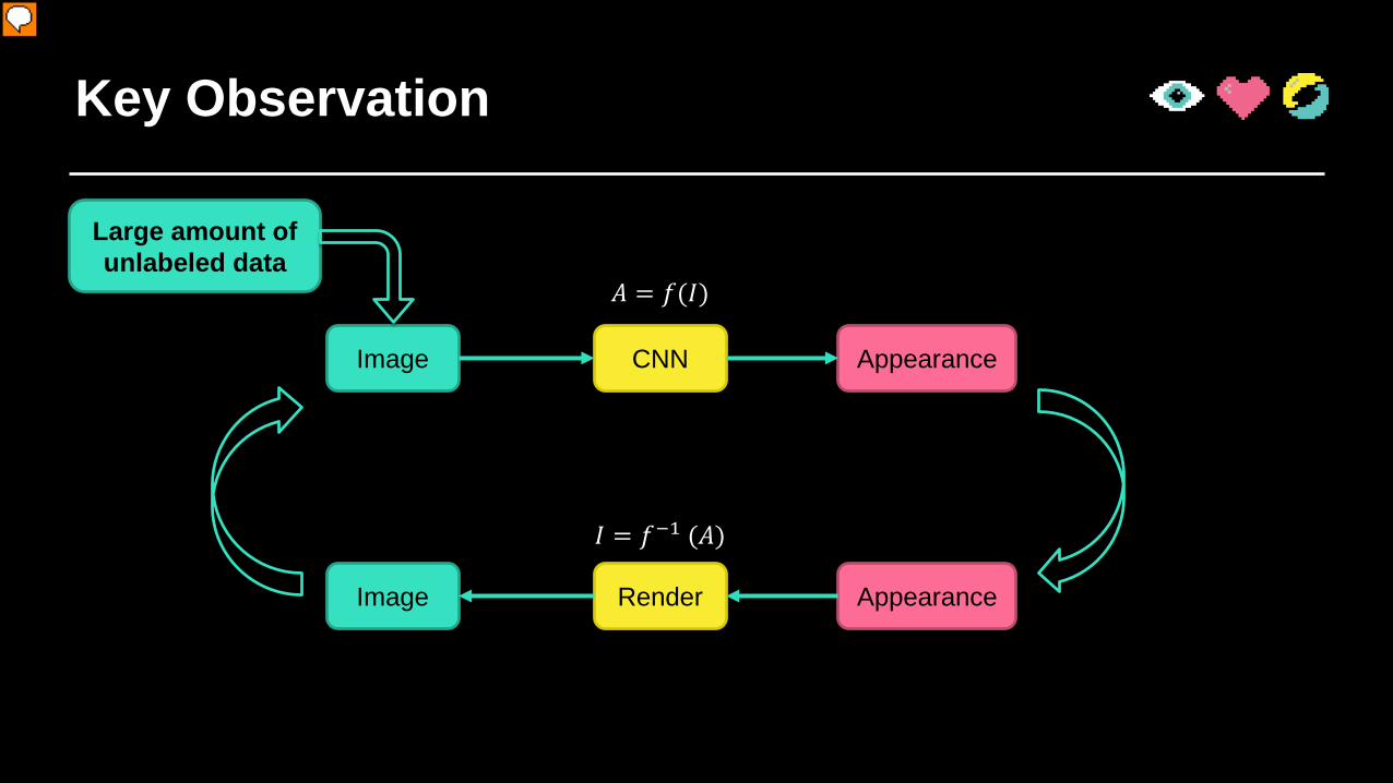
Large amount of unlabeled data
演示者
演示文稿备注
While with rendering as a known inverse mapping, we still need a large amount of appearance data, which is still not available. But as we mentioned, we have a lot of input natural texture image, without their corresponding appearance. (click) So we designed the self-augmented training scheme, utilize the known inverse and the large amount of unlabeled input to train our network.

Self-Augmented Training
Reference SVBRDF
CNN
Forward Prediction
LossBack propagation
Predicted SVBRDFInput Image
演示者
演示文稿备注
Now we explain detailed ideas of our self-augmented scheme. We first start from supervised training with few labeled data. (click)Here we got an image and its corresponded appearance data; to train the network, (click) we feed image to the network, got its prediction, (click) compare with ground truth reference to compute loss, finally we back-propagate and update the networks.
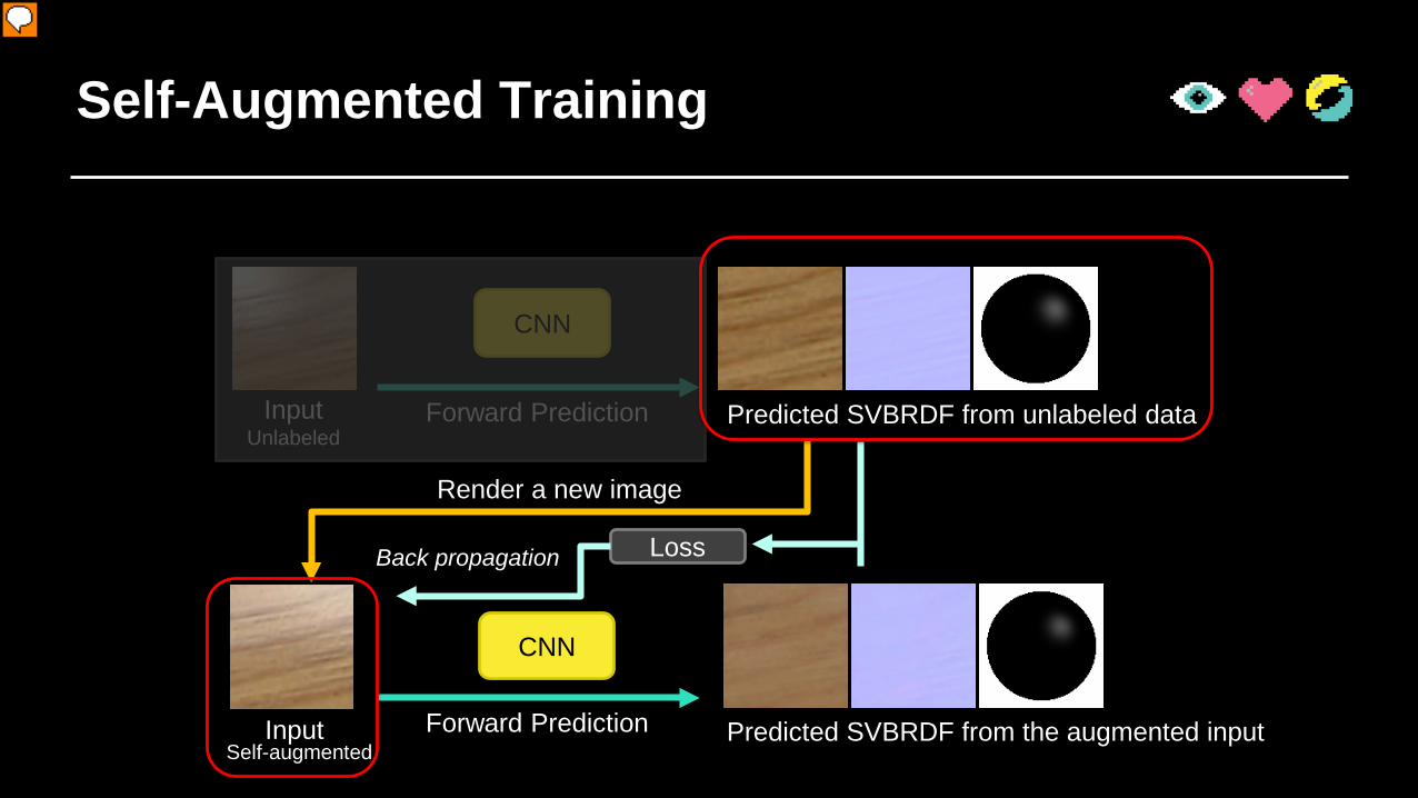
Self-Augmented Training
InputUnlabeled
Predicted SVBRDF from unlabeled data
CNN
Forward Prediction
Render a new image
CNN
Forward Prediction
LossBack propagation
Predicted SVBRDF from the augmented inputSelf-augmented
Input
演示者
演示文稿备注
Of course, few labeled data is not enough for training this task; and here is how our self-augment method helps us with unlabeled image. Giving one unlabeled image without ground truth appearance, (click) we feed it to the network and got predictions; (click) note this prediction, although it is an valid appearance, is not the ground truth appearance since the network still have error. However, remember our key observation that we have rendering as a known inverse mapping; so we could render a new input image using predicted appearance data. (click) Since the rendering is a “ground truth” process. We actually got a new pair of training data, with rendered image as input (click) and predicted appearance as ground truth (click). Finally, the CNN could be updated using this training pairs. (click) The training are altering between labeled training with only few labeled data and self-augmented training with large amount of unlabeled data. This is the pipeline of our self-augment training; we call it “self-augmented training” since the data is generated with the network itself on the fly during training.

1D illustration of Self-Augmentation
Image
BRDF parameters
Image
SVBRDF
演示者
演示文稿备注
In order to better illustrate the self-augmented scheme, here we show an illustration in 1D case. Suppose the x-dim is the output BRDF parameter, y-dim is the image input and the gray curve is the mapping we want to learn between image and appearance. (click); and we might got some labeled training data, here shows a example. Suppose we have sufficient label data, draw with green circle (click), we can well approximate the target function by supervised training and fit the mapping well, visualized as the yellow dashed curve (click). Please Note in real appearance cases a svbrdf material may paired with different image under different lighting conditions; here we just show a simplified version in 1D for a intuitive demonstration.

1D illustration of Self-Augmentation
BRDF parameters
Image
SVBRDF
Image
演示者
演示文稿备注
However, if we only have very few labeled data, the fitted mapping could not exactly match the mapping we want. For example, this figure shows the result with only three points; the fitted mapping is clearly biased from ground truth.
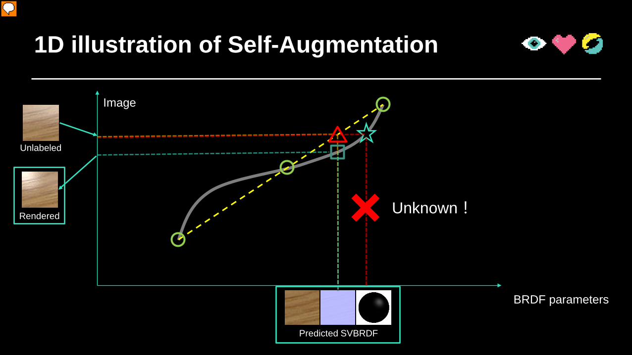
1D illustration of Self-Augmentation
BRDF parameters
Unlabeled
Predicted SVBRDF
Rendered Unknown!
Image
演示者
演示文稿备注
Now we show demonstration of our self-augmentation. (click) Given an unlabeled data, we first follow the current mapping (the yellow line) and we get an predicted appearance. Note this appearance is not the ground truth label of input unlabeled image; (click) the ground truth appearance should be found following the mapping visualized as gray curve, and we do not know it since it’s unlabeled. (click) But given this predicted appearance, since the inverse mapping is well defined by rendering, we could render a new image with this appearance. (click) So you could see that now we have got one “self augmented” labeled data pair, (click) with rendered image as input and previously predicted appearance as label.

1D illustration of Self-Augmentation
BRDF parameters
Unlabeled
Predicted SVBRDF
Rendered
Image
演示者
演示文稿备注
By using large collection of unlabeled data and our self-augmentation method, (click) we could progressively augmenting paired training data and finally help the fitting converge to our target mapping.

Why SA scheme works
• Exploring the meaningful domain • Defined in high dimensional space
BRDF parameters
Imag
e
演示者
演示文稿备注
The key of the self-augmentation scheme is exploring the meaningful domain of the output space that we are willing to explore. This is critical for tasks that output a high dimensional function, like a texture image. We are only interested in modeling natural textures, not for random noise liked non-sense textures. The self-augmented scheme, together with large amount of unlabeled data allow us to train the CNN that only for those natural textures defined by those unlabeled inputs.

The pitfall
• Local minimal / model collapsing– Interleave labeled & SA training minibatches
Imag
e
BRDF parameters
Unlabeled

Network StructureFully Convolutional, U-Net
FC1024
Imag
e in
put
BRDF
par
amet
ers
Homogeneousreflectance parameter estimation
256x
256x
1612
8x12
8x32
64x6
4x64
32x3
2x12
8
Spatially varying reflectance parameter estimation
16x1
6x25
68x
8x25
6
Imag
e in
put
256x
256x
1612
8x12
8x32
64x6
4x64
32x3
2x12
816
x16x
256
8x8x
256
8x8x
256
256x
256x
1612
8x12
8x32
64x6
4x64
32x3
2x12
816
x16x
256
SVBR
DF m
aps
Width x Height x Channel Convolution (3x3 kernel, stride 2) + BN + ReLUWidth x Height x Channel Bi-linear upsample + Convolution (3x3 kernel) + BN + ReLU
Hidden unit Fully connection layerLegend
演示者
演示文稿备注
Now we demonstrate some implementation details. As for the network structure, we use traditional convolution layers and fully connection layer to predict global BRDF parameters. For texture maps we use fully convolutional encoder-decoder structure with short cut links.

Training Details
• Training data– Wood / Metal / Plastic– 60 labeled SVBRDFs– 1000+ unlabeled photos– 256*256 patch
• Performance (Titan X)– Training: ~40 hours – Inference: ~0.3 sec.
Data and Source Code:http://msraig.info/~sanet/sanet.htm
演示者
演示文稿备注
As for training data, we trained our model on three dataset contains different type of materials: wood, metal, and plastic. For each dataset we ask artists modeled around 60 appearances and collect more than 1000 unlabeled images. The input image dimension is 256. We use caffe to build and train our models. Training took around 40 hours on a single Titan X GPU and inference for a single image took around 0.3 seconds. We have release our data and source code on our website, you could either access via the hyperlink, or scan the QR code on screen.

Results - WOOD
Input Albedo Normal Specular Novel lighting
Reference(Modeled by Artist)
演示者
演示文稿备注
Now we show our experiment results First we show our prediction on a wood sample. (click) We could see that our network provides a nice visually results. Still, we want to know that whether our result is really plausible. So we asked an experienced artist modeled this image for us. (click) This is artist modeled result. but overall, the results are plausible. Our results faithfully decomposed shading information contained in input and produced a clean diffuse texture;

Results - METAL
Input
Reference(Modeled by Artist)
Albedo Normal Specular Novel lighting
演示者
演示文稿备注
This is our predicted result on a metal material comparing with artist’s modeling. Similar to wood, we also get plausible results. Notice that our result recovered the bump details well even compared with artists’ result.

Results - PLASTIC
Input Albedo Normal Specular Novel lighting
Reference(Modeled by Artist)
演示者
演示文稿备注
This is our predicted result on a plastic result material comparing with artist’s modeling. Note in this input image, the highlight effect are combined with large bump normal effects. Nevertheless, our model also produced good results. The large normal bump varation are well captured; although compare with artists’ modeling, our recovered specular are a little bit sharper, but we still got plausible results under novel lighting.
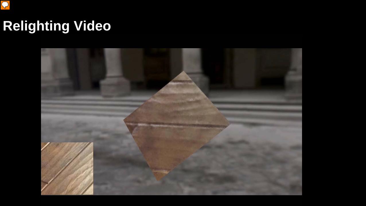
Relighting Video
演示者
演示文稿备注
Here, we show a video that renders our predicted appearance under an rotated lighting. The corresponded input image are shown on bottom-left. Generally, our method produces plausible visually appearance results under dynamic lighting conditions with only a single photograph as input.

SA-S
VBRD
F-ne
tSV
BRDF
-net
Input
Benefit of Self-Augmentation
WithSelf-Augmented
Training
WithoutSelf-Augmented
Training
演示者
演示文稿备注
Finally, we show benefit of our self-augmentation method. We trained our neural network with our self-augmentation scheme and without it, which means we only use few labeled data we get. For the input image on the left, the first row and second row show the prediction result with self-augmentation and without self-augmentation. Clearly, our self-augmented scheme utilized large information contained in unlabeled data and get better results; Without self-augmentation, the prediction will have artifacts, such as the “burn” spot in the diffuse texture, (click) and a significant larger specular (click).

BRDF-Net
• Manageable scale problem for better understanding
CNN
Homogeneous BRDFRendered on a sphere
Under environment lighting
Reflectance parameters
FC1024
Imag
e in
put
BRDF
par
amet
ers
Homogeneousreflectance parameter estimation
256x
256x
1612
8x12
8x32
64x6
4x64
32x3
2x12
8
16x1
6x25
68x
8x25
6
演示者
演示文稿备注
We can see our method do produces high quality results with minimal number of data. But we want to further explore how much labeled training data we can save. To perform such analysis, we need a more manageable scale problem. Here, we want to estimate the homogeneous reflectance parameters from a single input image. Since we only estimate limited number of parameters instead of a material maps, we can check the full space we want to recover and perform in-depth analysis.

BRDF-Net
• Effects of self-augmentation• Full labeled data vs Sparse labeled + unlabeled (rest)
演示者
演示文稿备注
Here we show the effect of self-augmentation by showing the estimation error map with different experiment setup. The bottom row shows the data point we used as labeled data, leaving the rest as unlabeled data. The top row shows results training without self-augmentation and the middle row shows results with self-augmentation training. The base line is trained with all the data points marked as labeled data, you can see that all the self-augmented training results produce good fit comparable to the baseline. Even in the extreme case that we only have only 8 labeled examples on the corner of the space, our results produce equal quality fitting as all the data marked as labeled data. On the contrary, without self-augmentation, the top row results shows very large estimation error.

BRDF-Net
• Effects of unlabeled data
演示者
演示文稿备注
Here we also test how the ratio between labeled and unlabeled data affects the training. We set the full space as 100 percent, different rows shows results with different number of labeled data, the columns shows different number of unlabeled data. You can see the error table is almost symmetrical, meaning that with the self-augmentation scheme, same percent of unlabeled data can ack very similar as labeled data. Proving the efficiency of the self-augmentation scheme.

Self-augmentation vs dual learning
• Parallel scheme– With different known components
Inpu
t
Out
put
CN
N
Traditional training
Inpu
t
Out
putC
NN
Dual learningC
NN
Inpu
t
Out
putC
NN
Self-augmentation
Ren
de r
演示者
演示文稿备注
You may feel like our scheme is similar to the dual learning. Actually, the self-augmented training and dual learning are two parallel technique that has similar general structure.

Self-augmentation vs dual learningIn
put
Out
put
CN
N
Traditional training
Inpu
t
Out
putC
NN
Rich data in both input and outputWith known mapping
Dual learningC
NN
Rich data in both input and outputLearn the mapping
?
Inpu
t
Out
putC
NN
Self-augmentation
Ren
der
Rich data only for input
演示者
演示文稿备注
For traditional training, for one forward task, it has rich data in both the input and output space, with known mapping between them. For Dual learning, it has rich data on both the input and output space, but trying to find the unknown connection between the two space, utilizing the cycle structure. While for our self-augmentation we only have rich data for the input, with the help of known rendering as inverse, we explore both the output space and the mapping between the input and output space.

Conclusion
• Self-augmented training– Single image => Plausible appearance – Labeled + Unlabeled training
• Future Work– More complex surface appearance– Self-augmentation for other tasks
演示者
演示文稿备注
In conclusion, we proposed a novel training scheme, named self-augmented training, for single image appearance estimation. Such scheme enable us training networks with a large collection of unlabeled images and reducing required amount of labeled data. We demonstrate our method’s benefit and did a lot of validation experiments. Our method do have some limitations; currently we only estimate appearance on planar surface with a homogeneous specular; Also, although we did some validation experiments on a manageable problem, we still lacking a very formal theoretical framework. As for future work, we would like extending our method handling more complex surface appearance and extending our method to other tasks sharing similar properties.

Acknowledgements
• Anonymous Reviewers• Beijing Film Academy• NSF grant: IIS-1350323
演示者
演示文稿备注
Finally, we want to thank all anonymous reviewers for their feed back; Beijing Film Academy for creating SVBRDF datasets and all the funding agencies.

THANKS!
演示者
演示文稿备注
Thank you very much for listening!

BACKUP SLIDES
演示者
演示文稿备注
Thank you for listening! Our paper, data and source code have been released, you might want to check our website for more details.

Self-augmentation vs dual learning
• Unlabeled Input• Known Inverse Mapping
• Unlabeled on two tasks• Trained dual tasks
Dual learningSelf-augmentation
Input AppearanceCNN
Render
Image A Image BCNN A-B
CNN B-A
演示者
演示文稿备注
Here we briefly discuss our relationship with a recently published machine learning method called dual learning and also latest cycle-GAN, dual-GAN scheme. the self-augmented training and dual learning are two parallel technique that has similar general structure. For traditional training, for one forward task, it has rich data in both the input and output space, with known mapping between them. For Dual learning, it has rich data on both the input and output space, but trying to find the unknown connection between the two space, utilizing the cycle structure. for our self-augmentation we only have rich data for the input (image), but not the output (SVBRDF). With the help of known rendering as inverse, we explore both the output space and the mapping between the input and output space.

Discussion
• Exploring the meaningful domain defined in high dimensional space
BRDF parameters
Imag
e
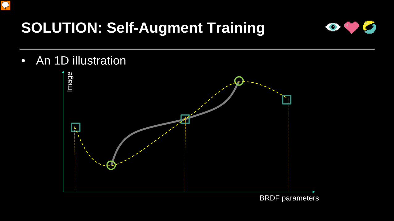
SOLUTION: Self-Augment Training
• An 1D illustrationIm
age
BRDF parameters
演示者
演示文稿备注
Notice that, this self-augmentation only works when the newly generated square is within the range we are willing to fit. If all the data points randomly generated without a unlabeled data, (click) we still got a poor fit. That is why the correct inverse mapping is critical: it help us to using unlabeled data to guide our data augmentation.
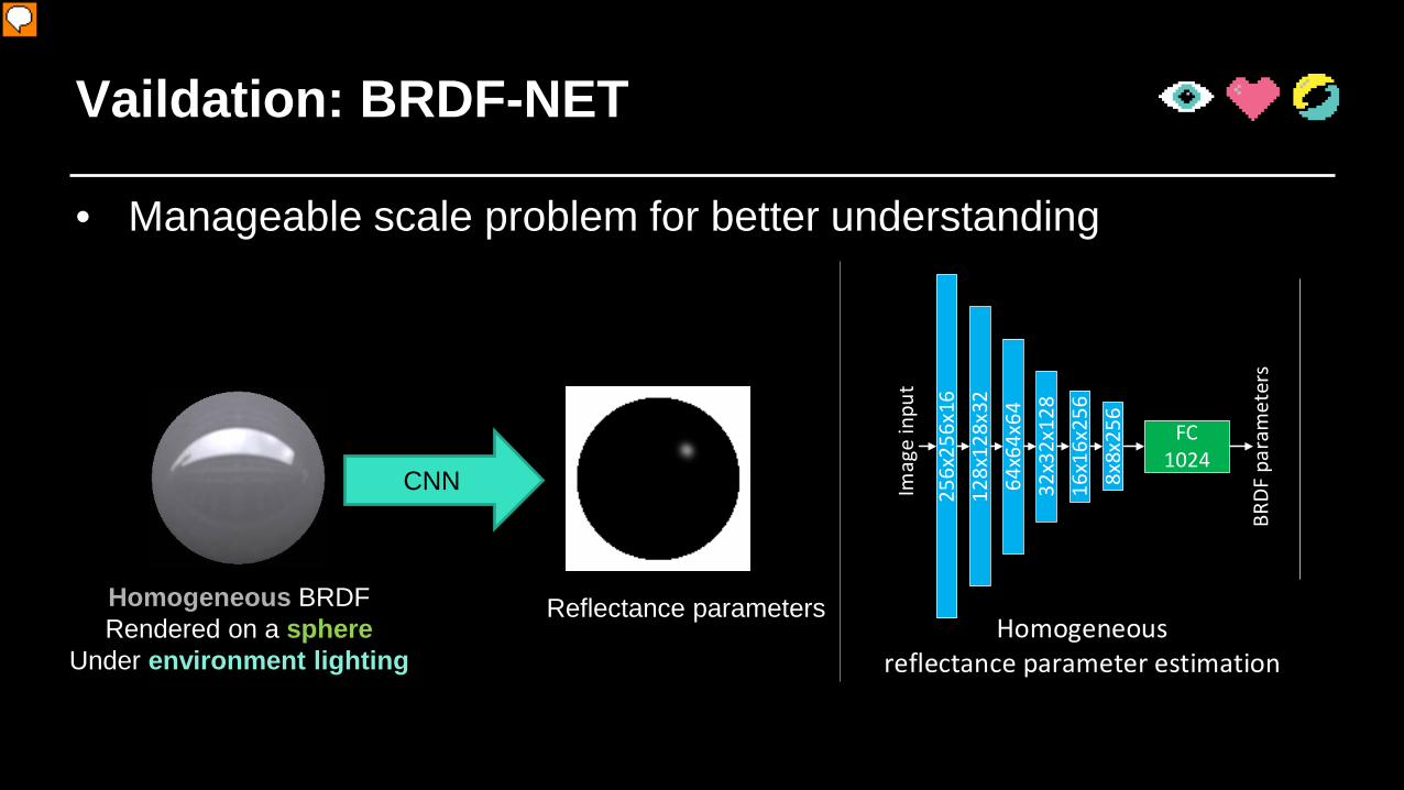
Vaildation: BRDF-NET
• Manageable scale problem for better understanding
CNN
Homogeneous BRDFRendered on a sphere
Under environment lighting
Reflectance parameters
FC1024
Imag
e in
put
BRDF
par
amet
ers
Homogeneousreflectance parameter estimation
256x
256x
1612
8x12
8x32
64x6
4x64
32x3
2x12
8
16x1
6x25
68x
8x25
6
演示者
演示文稿备注
Our experiments and results on Spatial-variant BRDF have shown that we could get plasuble results with a small amount of labeled data. Still, we want to further explore limits of our self-augmented scheme; to perform such analysis, we need a more manageable scale problem. Here we explore this with homongeneous appeance estmation – we want to estimate homogeneous reflectance parameters from a single input image. This is a problem that we could more easily check the full space we want to recover and perform some analysis.

Vaildation: BRDF-NET
• Effects of self-augmentation– Full labeled data v.s. sparse labeled + rest data unlabeled
演示者
演示文稿备注
First here we show the effect of self-augmentation by showing the estimation error map with different setup. The bottom row shows the data point we used as labeled data, leaving the rest as unlabeled data. The top row shows results training without self-augmentation and the middle row shows results with self-augmentation training. The baseline on topleft corner is trained with all the data points marked as labeled data. We could see that all the self-augmented training results produce good fit comparable to the baseline. Even in the extreme case that we only have only 8 labeled examples on the corner of the space, our results produce equal quality fitting as all the data marked as labeled data. On the contrary, when without self-augmentation, the top row results shows very large estimation error.

Vaildation: BRDF-NET
• Effects of different amount of unlabeled data
演示者
演示文稿备注
We also test how the ratio between labeled and unlabeled data affects the training. We set the full space as 100 percent, different rows shows results with different number of labeled data, the columns shows different number of unlabeled data. You can see the error table is almost symmetrical, meaning that with the self-augmentation scheme, same percent of unlabeled data can ack very similar as labeled data. Proving the efficiency of the self-augmentation scheme.

Vaildation: BRDF-NET
• Interleave training ratio between unlabeled / labeled data
演示者
演示文稿备注
Our self-augment training scheme still need few labeled training data interleaved feeding with unlabeled data when training. We also want to explore how this interleave ratio affects our training results. Here we show four different setups that varies from only use 5% of labeled training data to 70% labeled training data, leaving rest as unlabeled data, corrspoding to the 4 curves. The x axis corresponds to different interleave ratios; points to the left means labeled data are interleaved less, while points to right means more labeled data are interleaved. We could see that if interleave ratio is too high, the training would become unstable, especially when amount of labeled data are few; on the other hand, if set the ratio too low, the information from unlabeled data are leveraged less effieiently. Overall, an interleave ratio around 1 to 1 is often a good choice for self-augmentation scheme.

SOLUTION: Self-Augment Training
• An 1D training illustration– Regression with 2 layer MLP– Only 2 labeled data at the ends / unlabeled data for full range

Vaildation: BRDF-NET
• Vaildation on convex hull assumption
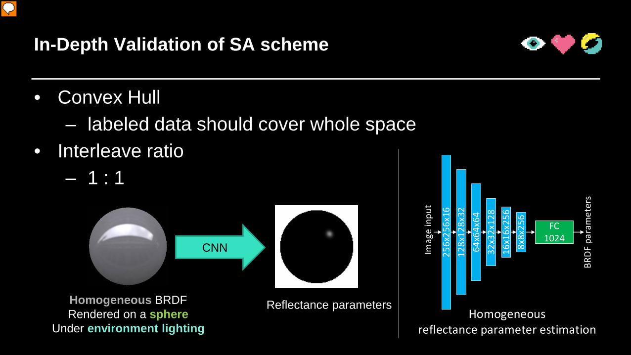
In-Depth Validation of SA scheme
• Convex Hull– labeled data should cover whole space
• Interleave ratio– 1 : 1
CNN
Homogeneous BRDFRendered on a sphere
Under environment lighting
Reflectance parameters
FC1024
Imag
e in
put
BRDF
par
amet
ers
Homogeneousreflectance parameter estimation
256x
256x
1612
8x12
8x32
64x6
4x64
32x3
2x12
8
16x1
6x25
68x
8x25
6
演示者
演示文稿备注
We also do some in-depth validation of our self-augmentation. Basically, some important results are: Our self-augmentation works best when the provided few labeled data covered whole sampling space. We do observe some extrapolation power, but the behavior would be undefined if input is too faraway from convex hull of labeled data. Also during training we do need to interleave providing labeled data pairs and unlabeled training pairs to stable training. The interleave ration is a trade-off between training’s stability and training performance; We empirically found that 1:1 is a good settings for most experiments. Due to time limit we will not discuss them in detail in this talk; please refer to our paper for detailed report.

Self-augmentation vs dual learning
Inpu
t
Out
put
CN
N
Traditional trainingIn
put
Out
putC
NN
Dual learning
CN
N
Inpu
t
Out
putC
NN
Self-augmentation
Ren
der
• Unlabeled Input• Known Inverse Mapping
• Unlabeled on two tasks• Trained dual tasks
演示者
演示文稿备注
Here we briefly discuss our relationship with a recently published machine learning method called dual learning. the self-augmented training and dual learning are two parallel technique that has similar general structure. For traditional training, for one forward task, it has rich data in both the input and output space, with known mapping between them. For Dual learning, it has rich data on both the input and output space, but trying to find the unknown connection between the two space, utilizing the cycle structure. for our self-augmentation we only have rich data for the input (image), but not the output (SVBRDF). With the help of known rendering as inverse, we explore both the output space and the mapping between the input and output space.
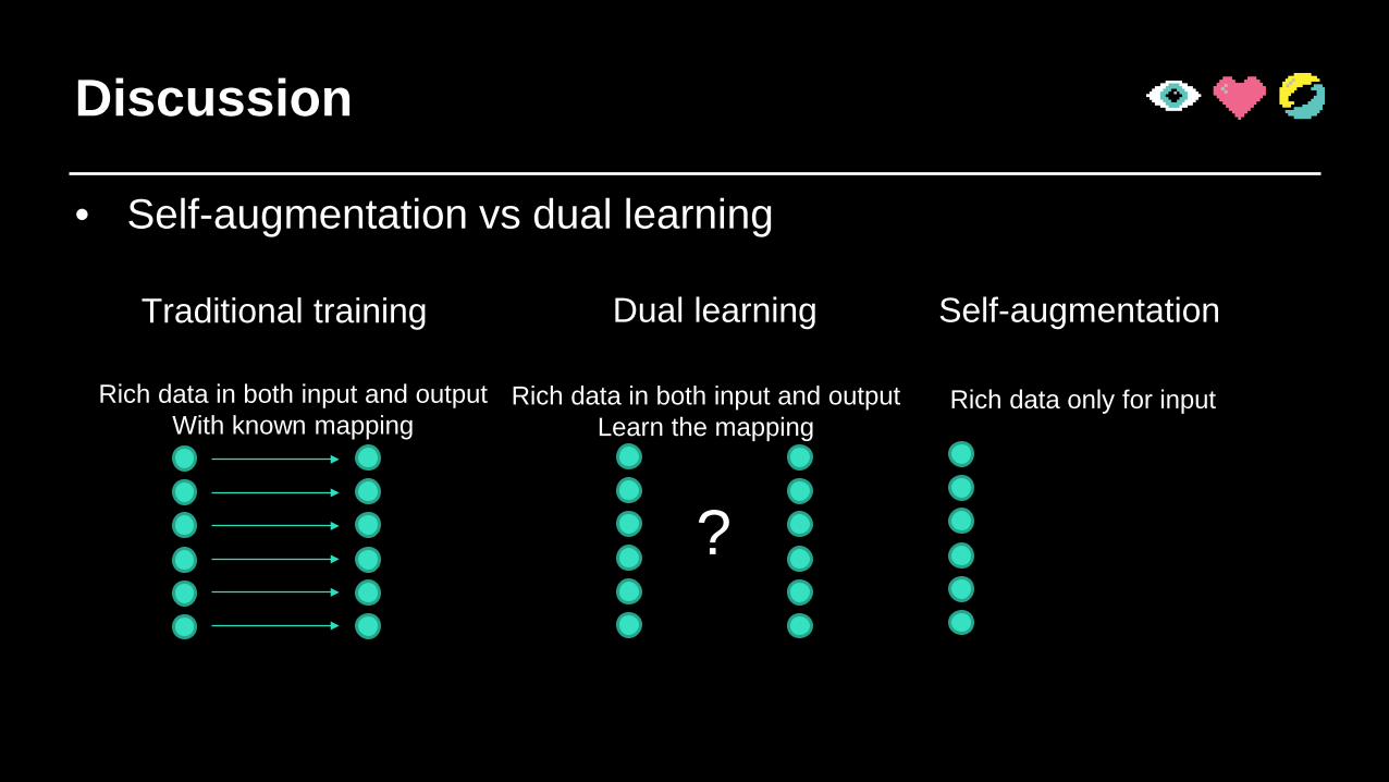
Discussion
• Self-augmentation vs dual learning
Rich data in both input and outputWith known mapping
Rich data in both input and outputLearn the mapping
?
Rich data only for input
Traditional training Dual learning Self-augmentation

Self-augmented training Dual learning
- Unlabeled on two sets- Trained dual tasks
Input AppearanceCNN
Render
Image A Image BCNN A-B
CNN B-A
Discussion
- Unlabeled input- Known inverse mapping
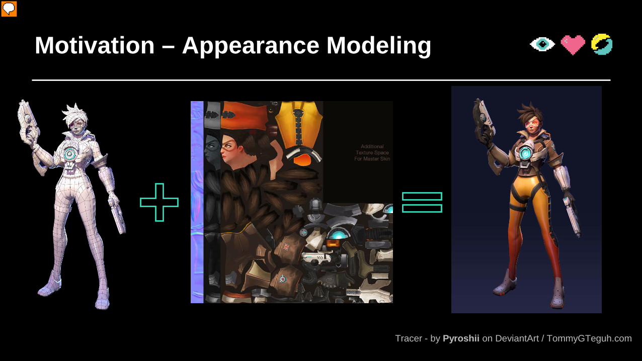
Motivation – Appearance Modeling
Tracer - by Pyroshii on DeviantArt / TommyGTeguh.com
演示者
演示文稿备注
Appearance plays a very important role in computer graphics and it is an essential component for 3D content creation, especially for gaming and movie industries.

Modeling Appearance by CNN
Input Image
Albedo Map Bump Map
Homogeneous Specular(Ward Model)
Spatially varying reflectance parameter estimation
Imag
e in
put
256x
256x
1612
8x12
8x32
64x6
4x64
32x3
2x12
816
x16x
256
8x8x
256
8x8x
256
256x
256x
1612
8x12
8x32
64x6
4x64
32x3
2x12
816
x16x
256
SVBR
DF m
aps
FC1024
Imag
e in
put
BRDF
par
amet
ers
Homogeneousreflectance parameter estimation
256x
256x
1612
8x12
8x32
64x6
4x64
32x3
2x12
8
16x1
6x25
68x
8x25
6
演示者
演示文稿备注
Artist modeling appearance by their own knowledge; Motivated by this, we choose to using Deep Learning method. Given a single image input, we use conv. Nerual network to output our predictions: a spatial-variant albedo map; a spatial-variant bump normal map, and parameters representing a homogeneous BRDF. We choose to only output a homogeneous BRDF value for whole image since appearance from single image is essentially a ill-posed problem, and in many cases a homogeneous BRDF already output plausible results.
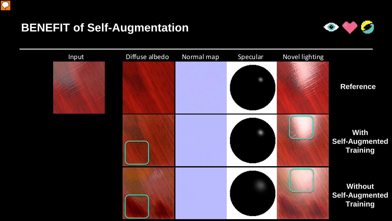
BENEFIT of Self-Augmentation
Input Diffuse albedo Normal map Specular Novel lighting
Refe
renc
eSA
-SVB
RDF-
net
SVBR
DF-n
et
Reference
WithSelf-Augmented
Training
WithoutSelf-Augmented
Training
演示者
演示文稿备注
Finally, we show benefit of our self-augmentation method. We trained our neural network with our self-augmentation scheme and without it, which means we only use few labeled data we get. The first row is a reference ground truth; The second row and third row show a comparison, with self-augmentation (click) and without self-augmentation (click). Clearly, our self-augmented scheme utilized large information contained in unlabeled data and get better results; Without self-augmentation, the prediction will have artifacts, such as the “burn ” spot in the diffuse texture, (click) and a significant larger specular (click).