Mon. Not. R. Astron. Soc. 000, 000–000 (0000) Printed Monday 23rd June, 2014 (MN LATEX style file v2.2)

A 3D extinction map of the Northern Galactic Plane based onIPHAS photometry

S. E. Sale1, J. E. Drew2, G. Barentsen2, H. J. Farnhill2, R. Raddi3, M. J. Barlow4,J. Eisloffel5, J. S. Vink6, P. Rodrıguez-Gil7,8, N. J. Wright21 Rudolf Peierls Centre for Theoretical Physics, Keble Road, Oxford OX1 3NP, U.K.2 School of Physics, Astronomy & Mathematics, University of Hertfordshire, College Lane, Hatfield, Hertfordshire, AL10 9AB, U.K3 Department of Physics, University of Warwick, Gibbet Hill Road, Coventry, CV4 7AL, U.K4 University College London, Department of Physics & Astronomy, Gower Street, London WC1E 6BT, U.K.5 Thuringer Landessternwarte, Sternwarte 5, 07778, Tautenburg, Germany6 Armagh Observatory, College Hill, Armagh, Northern Ireland, BT61 9DG, U.K.7 Instituto de Astrofısica de Canarias, Vıa Lactea, s/n, La Laguna, E-38205, Santa Cruz de Tenerife, Spain8 Departamento de Astrofısica, Universidad de La Laguna, La Laguna, E-38204, Santa Cruz de Tenerife, Spain

Received .........., Accepted...........

ABSTRACTWe present a three dimensional map of extinction in the Northern Galactic Plane derived usingphotometry from the IPHAS survey. The map has fine angular (∼ 10 ′) and distance (100 pc)sampling allied to a significant depth (& 5 kpc). We construct the map using a method basedon a hierarchical Bayesian model as previously described by Sale (2012). In addition to meanextinction, we also measure differential extinction, which arises from the fractal nature of theISM, and show that it will be the dominant source of uncertainty in estimates of extinction tosome arbitrary position. The method applied also furnishes us with photometric estimates ofthe distance, extinction, effective temperature, surface gravity, and mass for∼ 38 million stars.Both the extinction map and the catalogue of stellar parameters are made publicly availablevia http://www.iphas.org/extinction.

Key words: ISM: dust, extinction – ISM: structure – stars: fundamental parameters – surveys

1 INTRODUCTION

Dust is a significant component of the plane of the Milky Way,essential to the cycling of matter between successive generationsof stars, while also posing an observational challenge through theprogressive extinction of starlight. Both stars and interstellar dustfollow their own distributions within the disk of the Galaxy – dis-tributions that we wish to establish to some accuracy in order to un-derstand how the Galaxy has been built and will evolve. The majorconcentration of Galactic dust is within 100 pc or so of the Galacticplane (Marshall et al. 2006), along with the majority of stars (Juricet al. 2008). So far we have only a poor grasp of how extinctionbuilds up as a function of distance away from the Sun, even if therehas been good progress at far IR wavelengths in determining totaldust columns according to sightline (Schlegel et al. 1998; PlanckCollaboration et al. 2013).

Mapping extinction in three dimensions both removes a nui-sance factor for astrophysical studies and enables the determinationof the dust distribution within the Galactic disk and the physicalprocesses shaping it. Observations of the gas phases of the inter-stellar medium (ISM) and dust in continuous emission necessarilyintegrate over the entire column out to the ‘edge’ of the Galaxy– unsupported, such data cannot directly map three dimensional

structures. In significant contrast, extinction only depends on thedust column between us and the very many observed stars, whichappear at a range of distances. Accordingly, the systematic mea-surement of extinction to a large number of stars can offer an un-usually direct route to the three dimensional structure of the ISM.Our location within the Galaxy means that we can study its ISM infar greater detail than that of any other galaxy. The knowledge wegain from studying our own Galaxy can subsequently be applied toothers.

The history of extinction mapping extends back to Trumpler(1930). More recently, Neckel & Klare (1980) used observations of11,000 stars to map extinction near the Galactic Plane, whilst Are-nou, Grenon & Gomez (1992) used the INCA database of 215,000stars to constrain a 3D model of extinction. The recent growthin survey astronomy and the resulting explosion in the volume ofavailable data has facilitated extinction mapping, enabling signifi-cant improvements in depth, precision and accuracy. Marshall et al.(2006) used 2MASS observations of red giant stars to map extinc-tion in the inner Galaxy. Majewski, Zasowski & Nidever (2011)paired 2MASS and GLIMPSE data, whilst Berry et al. (2012) usedSDSS in conjunction with 2MASS. Vergely et al. (2010) and Lalle-ment et al. (2014) have applied geophysical techniques from Taran-tola & Valette (1982) to map the local ISM. Sale (2012) presented

c© 0000 RAS

arX

iv:1

406.

0009

v3 [

astr

o-ph

.GA

] 2

0 Ju

n 20

14

2 Sale et al.

a method for mapping extinction using a hierarchical Bayesianmodel, simultaneously estimating the distance extinction relation-ship and the properties of the stars along the line of sight. Subse-quently Green et al. (2014) have proposed a similar method.

The INT/WFC Photometric Hα Survey of the northern Galac-tic Plane (IPHAS; Drew et al. 2005) is the first comprehensivedigital survey of the northern Galactic disc (|b| 6 5◦), covering aGalactic longitude range of 30◦ . l . 215◦. Imaging is performedin the r, i and Hα bands down to r ∼ 20. As demonstrated by Sale(2012), the IPHAS photometric system is unusually well suited tobreaking the degeneracy between extinction and effective temper-ature: the (r−Hα) colour is effectively a proxy for Hα equivalentwidth, and thus effective temperature, and is less heavily influencedby extinction.

An initial public data release of IPHAS data obtained beforethe end of 2005 was previously made available (Gonzalez-Solareset al. 2008). Since then, the entire survey area has been observedat least once, leaving only 8% of the footprint still wanting survey-standard photometry. Furthermore, a global photometric calibrationof all IPHAS data has recently been completed. A second data re-lease (IPHAS DR2) containing both the additional data and the newglobal photometric calibration of understood precision is describedby Barentsen et al. (2014). Sale et al. (2009) demonstrated thatattempting to map extinction using inconsistently-calibrated datawould inevitably lead to results exhibiting erratic biases. However,now that a global photometric calibration is in hand it is possible toutilise the IPHAS DR2 catalogue to map 3D extinction across theentire northern Galactic Plane at high angular resolution for the firsttime. The aim of this paper is to apply the method of Sale (2012) toachieve this mapping.

The organisation of this paper is as follows. Section 2 sum-marises the method employed, concentrating on departures fromSale (2012) and details particularly relevant to the large scale im-plementation we perform here. In section 3 we present the 3D ex-tinction map alongside examples of derived stellar parameters. Wethen compare our extinction map to those of Marshall et al. (2006)and Schlegel et al. (1998), before closing with a discussion of themap produced here and future work.

2 METHOD

Sale (2012) proposed a method for simultaneously mapping ex-tinction and determining stellar parameters using a hierarchicalBayesian model. The Markov Chain Monte Carlo (MCMC) basedalgorithm, called H-MEAD (hierarchically mapping extinctionagainst distance), simultaneously estimates the distance-extinctionrelationship along a line of sight and the properties of the starssampled. The first step in this is to define an angular resolutionelement – an area on the sky for which we wish to find a distance-extinction relationship. Then, for each angular resolution element,we create a series of voxels1 by dividing the conical volume pro-jected onto each 2D angular resolution element into distance slices,each 100 pc in depth. We then employ IPHAS photometry of starswithin the angular resolution element as the means to estimate thedistance-extinction relationship as well as the characteristics of thestars.

Dust in the ISM is shaped by turbulent flows, that form frac-tal structures within the ISM across a range of scales from kpc to

1 a voxel is conventionally a volume pixel

∼ 100 km (Spangler & Gwinn 1990; Chepurnov & Lazarian 2010).This gives rise to differential extinction: since the dust density islikely to vary on very small scales – even within an already smallbut finite angular element – extinction to a given distance (or voxel)will take a range of values. The treatment of Sale (2012) includesdifferential extinction in the statistical model, accounting for its in-fluence on observations and enabling it to be measured for the firsttime. This is a key advance relative to many other extinction map-ping techniques, such as those of Marshall et al. (2006) and Greenet al. (2014).

Formally, H-MEAD estimates the posterior distribution

P(xxx, AAA|yyy) ∝ P(yyy|xxx)P(xxx|AAA)P(AAA), (1)

where xxx represents the properties of the stars within the an-gular resolution element, including distance, extinction, stellareffective temperature, surface gravity and metallicity. AAA is thedistance-extinction relationship, where the extinction to a givenvoxel at a given distance is described by a lognormal distribution,parametrized by a mean extinction and a standard deviation. As ashorthand we will refer to the standard deviation of the extinctionto a given voxel as the differential extinction. Finally yyy representsthe observations we have – in this case photometry from the IPHASDR2 catalogue. Therefore, we are attempting to find the posteriorprobability distribution of the stellar properties and the extinction-distance relationship consistent with the IPHAS DR2 catalogue. Byrepeating this analysis for many angular resolution elements we ac-quire a large 3D map of extinction.

The relationship between yyy and xxx is dependent on a set ofisochrones, we employ those of Bressan et al. (2012), and an ex-tinction law, in this case the RV = 3.1 law of Fitzpatrick & Massa(2007). P(xxx|AAA) includes priors on the distance, age, mass andmetallicity of stars. These arise from an assumed stellar density,star formation history, initial mass function and a probabilistic de-pendence of metallicity on Galactocentric radius. The priors aredescribed in more detail in Sale (2012). We note here that they areconservative and not overly constraining (e.g. they include a con-stant star formation rate over the history of the disk, plausible scale-lengths and heights). In general, the only constraint given by P(AAA)is that mean extinction should increase with respect to distance –although, as discussed in section 2.2, for the most distant voxels itis necessary to impose an additional constraint.

2.1 Angular resolution

The area density of stars varies substantially across the IPHAS sur-vey area due to variations in the three dimensional distribution ofboth dust and stars. Typically the angular distribution of stars isat its densest at lower Galactic longitudes (i.e. nearer the Galac-tic centre) and a few degrees removed from the Galactic Plane. Inthis inner Galactic region the three dimensional stellar density ishigh, whilst the dust, having a shorter scale height than the stars,obscures many stars near the midplane. The observed stellar den-sity is lowest either near the Anticentre or in regions of very strongextinction.

There is no clear and absolute standard by which we should setthe angular resolution of our map. There exists a tension betweenfiner resolutions which capture the fractal ISM in better detail and acoarser map which will reach a somewhat greater extinction depthand is more robust against the inclusion of poor data. This balanceclearly shifts between regions of high stellar column density, wherefiner resolutions are more feasible, and less densely populated re-gions, where we have to opt for lower resolutions. Consequently in

c© 0000 RAS, MNRAS 000, 000–000

A 3D extinction map of the Northern Galactic Plane 3

30

60

90

120

150

180

210

l

−5 0 5

b

5 10

15

30

60

resolution/arcmin

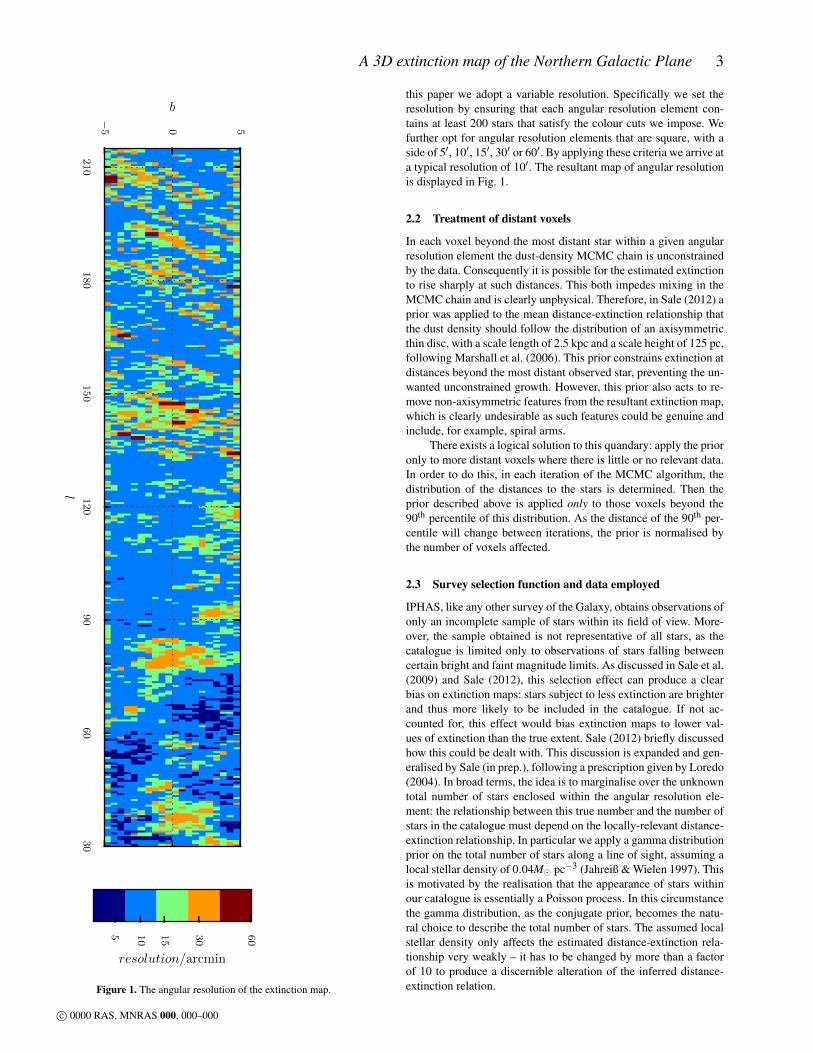
Figure 1. The angular resolution of the extinction map.

this paper we adopt a variable resolution. Specifically we set theresolution by ensuring that each angular resolution element con-tains at least 200 stars that satisfy the colour cuts we impose. Wefurther opt for angular resolution elements that are square, with aside of 5′, 10′, 15′, 30′ or 60′. By applying these criteria we arrive ata typical resolution of 10′. The resultant map of angular resolutionis displayed in Fig. 1.

2.2 Treatment of distant voxels

In each voxel beyond the most distant star within a given angularresolution element the dust-density MCMC chain is unconstrainedby the data. Consequently it is possible for the estimated extinctionto rise sharply at such distances. This both impedes mixing in theMCMC chain and is clearly unphysical. Therefore, in Sale (2012) aprior was applied to the mean distance-extinction relationship thatthe dust density should follow the distribution of an axisymmetricthin disc, with a scale length of 2.5 kpc and a scale height of 125 pc,following Marshall et al. (2006). This prior constrains extinction atdistances beyond the most distant observed star, preventing the un-wanted unconstrained growth. However, this prior also acts to re-move non-axisymmetric features from the resultant extinction map,which is clearly undesirable as such features could be genuine andinclude, for example, spiral arms.

There exists a logical solution to this quandary: apply the prioronly to more distant voxels where there is little or no relevant data.In order to do this, in each iteration of the MCMC algorithm, thedistribution of the distances to the stars is determined. Then theprior described above is applied only to those voxels beyond the90th percentile of this distribution. As the distance of the 90th per-centile will change between iterations, the prior is normalised bythe number of voxels affected.

2.3 Survey selection function and data employed

IPHAS, like any other survey of the Galaxy, obtains observations ofonly an incomplete sample of stars within its field of view. More-over, the sample obtained is not representative of all stars, as thecatalogue is limited only to observations of stars falling betweencertain bright and faint magnitude limits. As discussed in Sale et al.(2009) and Sale (2012), this selection effect can produce a clearbias on extinction maps: stars subject to less extinction are brighterand thus more likely to be included in the catalogue. If not ac-counted for, this effect would bias extinction maps to lower val-ues of extinction than the true extent. Sale (2012) briefly discussedhow this could be dealt with. This discussion is expanded and gen-eralised by Sale (in prep.), following a prescription given by Loredo(2004). In broad terms, the idea is to marginalise over the unknowntotal number of stars enclosed within the angular resolution ele-ment: the relationship between this true number and the number ofstars in the catalogue must depend on the locally-relevant distance-extinction relationship. In particular we apply a gamma distributionprior on the total number of stars along a line of sight, assuming alocal stellar density of 0.04M� pc−3 (Jahreiß & Wielen 1997). Thisis motivated by the realisation that the appearance of stars withinour catalogue is essentially a Poisson process. In this circumstancethe gamma distribution, as the conjugate prior, becomes the natu-ral choice to describe the total number of stars. The assumed localstellar density only affects the estimated distance-extinction rela-tionship very weakly – it has to be changed by more than a factorof 10 to produce a discernible alteration of the inferred distance-extinction relation.

c© 0000 RAS, MNRAS 000, 000–000

4 Sale et al.

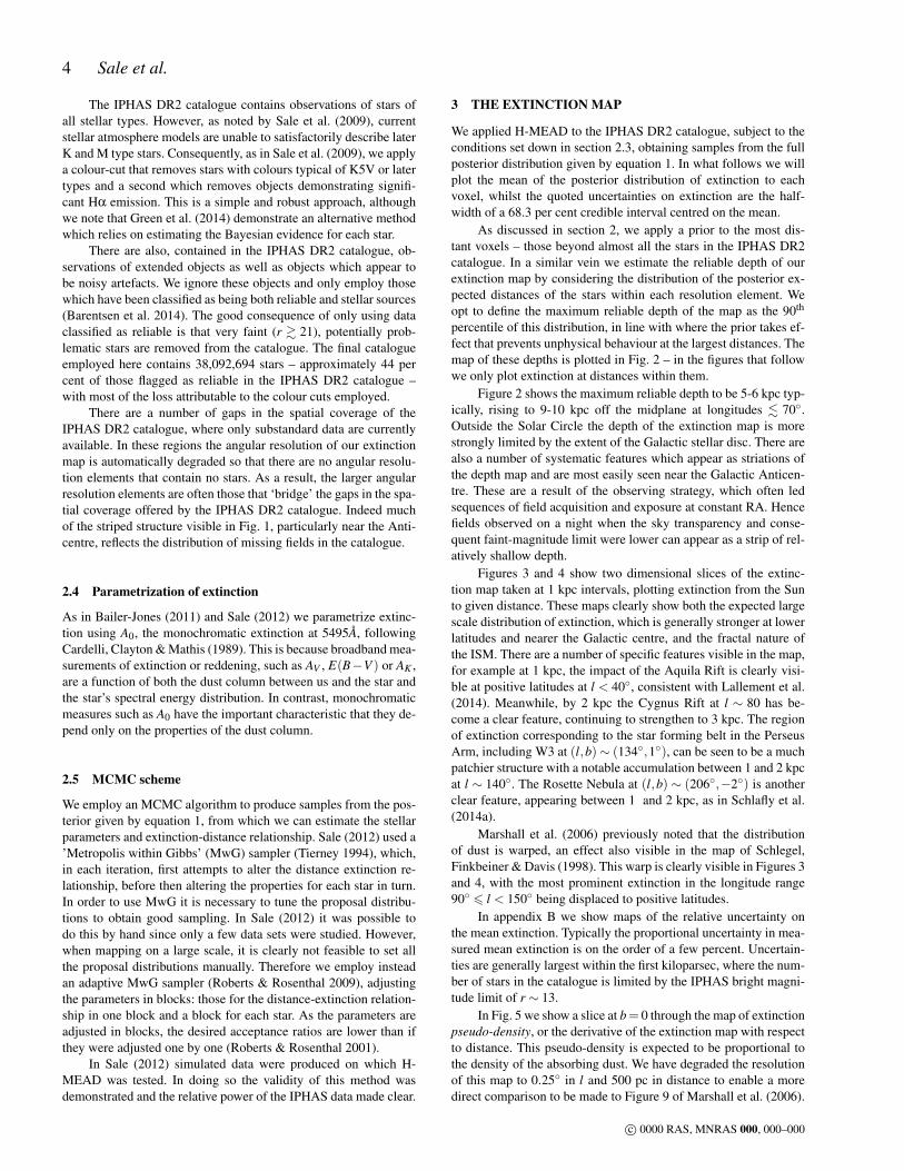
The IPHAS DR2 catalogue contains observations of stars ofall stellar types. However, as noted by Sale et al. (2009), currentstellar atmosphere models are unable to satisfactorily describe laterK and M type stars. Consequently, as in Sale et al. (2009), we applya colour-cut that removes stars with colours typical of K5V or latertypes and a second which removes objects demonstrating signifi-cant Hα emission. This is a simple and robust approach, althoughwe note that Green et al. (2014) demonstrate an alternative methodwhich relies on estimating the Bayesian evidence for each star.

There are also, contained in the IPHAS DR2 catalogue, ob-servations of extended objects as well as objects which appear tobe noisy artefacts. We ignore these objects and only employ thosewhich have been classified as being both reliable and stellar sources(Barentsen et al. 2014). The good consequence of only using dataclassified as reliable is that very faint (r & 21), potentially prob-lematic stars are removed from the catalogue. The final catalogueemployed here contains 38,092,694 stars – approximately 44 percent of those flagged as reliable in the IPHAS DR2 catalogue –with most of the loss attributable to the colour cuts employed.

There are a number of gaps in the spatial coverage of theIPHAS DR2 catalogue, where only substandard data are currentlyavailable. In these regions the angular resolution of our extinctionmap is automatically degraded so that there are no angular resolu-tion elements that contain no stars. As a result, the larger angularresolution elements are often those that ‘bridge’ the gaps in the spa-tial coverage offered by the IPHAS DR2 catalogue. Indeed muchof the striped structure visible in Fig. 1, particularly near the Anti-centre, reflects the distribution of missing fields in the catalogue.

2.4 Parametrization of extinction

As in Bailer-Jones (2011) and Sale (2012) we parametrize extinc-tion using A0, the monochromatic extinction at 5495A, followingCardelli, Clayton & Mathis (1989). This is because broadband mea-surements of extinction or reddening, such as AV , E(B−V ) or AK ,are a function of both the dust column between us and the star andthe star’s spectral energy distribution. In contrast, monochromaticmeasures such as A0 have the important characteristic that they de-pend only on the properties of the dust column.

2.5 MCMC scheme

We employ an MCMC algorithm to produce samples from the pos-terior given by equation 1, from which we can estimate the stellarparameters and extinction-distance relationship. Sale (2012) used a’Metropolis within Gibbs’ (MwG) sampler (Tierney 1994), which,in each iteration, first attempts to alter the distance extinction re-lationship, before then altering the properties for each star in turn.In order to use MwG it is necessary to tune the proposal distribu-tions to obtain good sampling. In Sale (2012) it was possible todo this by hand since only a few data sets were studied. However,when mapping on a large scale, it is clearly not feasible to set allthe proposal distributions manually. Therefore we employ insteadan adaptive MwG sampler (Roberts & Rosenthal 2009), adjustingthe parameters in blocks: those for the distance-extinction relation-ship in one block and a block for each star. As the parameters areadjusted in blocks, the desired acceptance ratios are lower than ifthey were adjusted one by one (Roberts & Rosenthal 2001).

In Sale (2012) simulated data were produced on which H-MEAD was tested. In doing so the validity of this method wasdemonstrated and the relative power of the IPHAS data made clear.

3 THE EXTINCTION MAP

We applied H-MEAD to the IPHAS DR2 catalogue, subject to theconditions set down in section 2.3, obtaining samples from the fullposterior distribution given by equation 1. In what follows we willplot the mean of the posterior distribution of extinction to eachvoxel, whilst the quoted uncertainties on extinction are the half-width of a 68.3 per cent credible interval centred on the mean.

As discussed in section 2, we apply a prior to the most dis-tant voxels – those beyond almost all the stars in the IPHAS DR2catalogue. In a similar vein we estimate the reliable depth of ourextinction map by considering the distribution of the posterior ex-pected distances of the stars within each resolution element. Weopt to define the maximum reliable depth of the map as the 90th

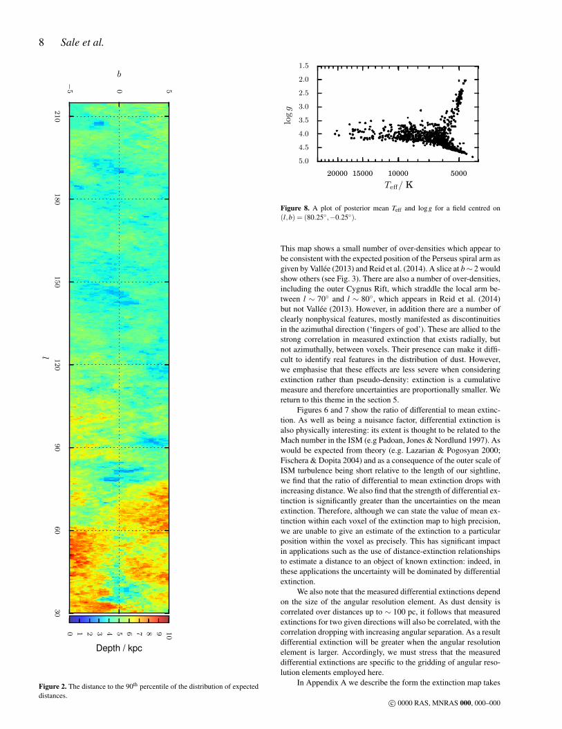
percentile of this distribution, in line with where the prior takes ef-fect that prevents unphysical behaviour at the largest distances. Themap of these depths is plotted in Fig. 2 – in the figures that followwe only plot extinction at distances within them.

Figure 2 shows the maximum reliable depth to be 5-6 kpc typ-ically, rising to 9-10 kpc off the midplane at longitudes . 70◦.Outside the Solar Circle the depth of the extinction map is morestrongly limited by the extent of the Galactic stellar disc. There arealso a number of systematic features which appear as striations ofthe depth map and are most easily seen near the Galactic Anticen-tre. These are a result of the observing strategy, which often ledsequences of field acquisition and exposure at constant RA. Hencefields observed on a night when the sky transparency and conse-quent faint-magnitude limit were lower can appear as a strip of rel-atively shallow depth.

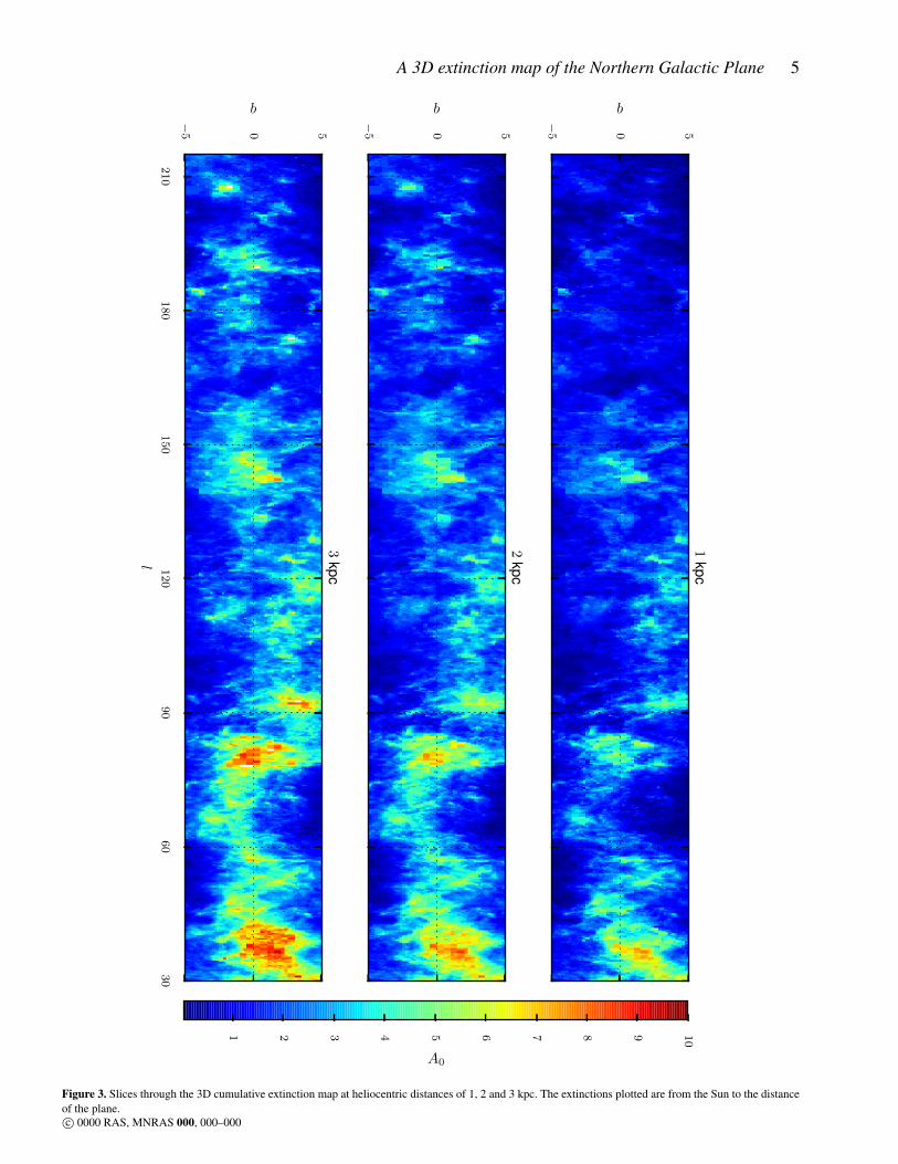
Figures 3 and 4 show two dimensional slices of the extinc-tion map taken at 1 kpc intervals, plotting extinction from the Sunto given distance. These maps clearly show both the expected largescale distribution of extinction, which is generally stronger at lowerlatitudes and nearer the Galactic centre, and the fractal nature ofthe ISM. There are a number of specific features visible in the map,for example at 1 kpc, the impact of the Aquila Rift is clearly visi-ble at positive latitudes at l < 40◦, consistent with Lallement et al.(2014). Meanwhile, by 2 kpc the Cygnus Rift at l ∼ 80 has be-come a clear feature, continuing to strengthen to 3 kpc. The regionof extinction corresponding to the star forming belt in the PerseusArm, including W3 at (l,b)∼ (134◦,1◦), can be seen to be a muchpatchier structure with a notable accumulation between 1 and 2 kpcat l ∼ 140◦. The Rosette Nebula at (l,b) ∼ (206◦,−2◦) is anotherclear feature, appearing between 1 and 2 kpc, as in Schlafly et al.(2014a).

Marshall et al. (2006) previously noted that the distributionof dust is warped, an effect also visible in the map of Schlegel,Finkbeiner & Davis (1998). This warp is clearly visible in Figures 3and 4, with the most prominent extinction in the longitude range90◦ 6 l < 150◦ being displaced to positive latitudes.

In appendix B we show maps of the relative uncertainty onthe mean extinction. Typically the proportional uncertainty in mea-sured mean extinction is on the order of a few percent. Uncertain-ties are generally largest within the first kiloparsec, where the num-ber of stars in the catalogue is limited by the IPHAS bright magni-tude limit of r ∼ 13.

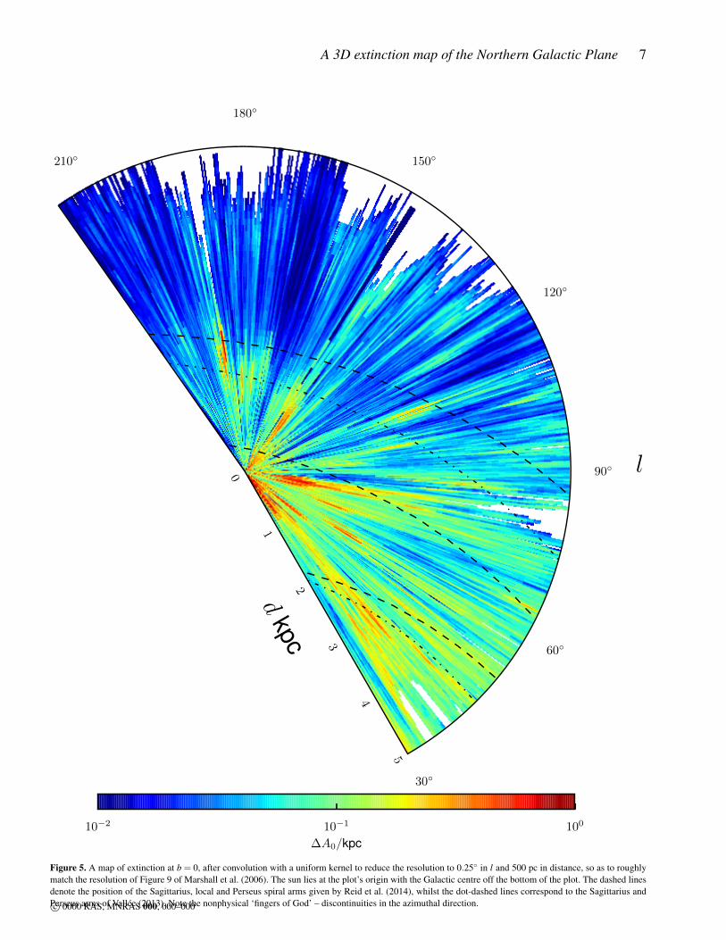
In Fig. 5 we show a slice at b= 0 through the map of extinctionpseudo-density, or the derivative of the extinction map with respectto distance. This pseudo-density is expected to be proportional tothe density of the absorbing dust. We have degraded the resolutionof this map to 0.25◦ in l and 500 pc in distance to enable a moredirect comparison to be made to Figure 9 of Marshall et al. (2006).

c© 0000 RAS, MNRAS 000, 000–000

A 3D extinction map of the Northern Galactic Plane 5

−5 0 5

b

1kpc

−5 0 5

b

2kpc

30

60

90

120

150

180

210

l

−5 0 5

b

3kpc

1 2 3 4 5 6 7 8 9 10

A0

Figure 3. Slices through the 3D cumulative extinction map at heliocentric distances of 1, 2 and 3 kpc. The extinctions plotted are from the Sun to the distanceof the plane.c© 0000 RAS, MNRAS 000, 000–000

6 Sale et al.

−5 0 5

b

4kpc

−5 0 5

b

5kpc

30

60

90

120

150

180

210

l

−5 0 5

b

6kpc

1 2 3 4 5 6 7 8 9 10

A0

Figure 4. Slices through the 3D cumulative extinction map at heliocentric distances of 4, 5 and 6 kpc. As in Fig. 3, we plot extinction from the Sun to thedistance of the plane. The white regions are those where we are beyond the maximum reliable distance for that angular resolution element.

c© 0000 RAS, MNRAS 000, 000–000

A 3D extinction map of the Northern Galactic Plane 7

30◦

60◦

90◦

120◦

150◦

180◦

210◦

0

1

2

3

4

5

dkpcl

10−2 10−1 100

∆A0/kpc

Figure 5. A map of extinction at b = 0, after convolution with a uniform kernel to reduce the resolution to 0.25◦ in l and 500 pc in distance, so as to roughlymatch the resolution of Figure 9 of Marshall et al. (2006). The sun lies at the plot’s origin with the Galactic centre off the bottom of the plot. The dashed linesdenote the position of the Sagittarius, local and Perseus spiral arms given by Reid et al. (2014), whilst the dot-dashed lines correspond to the Sagittarius andPerseus arms of Vallee (2013). Note the nonphysical ‘fingers of God’ – discontinuities in the azimuthal direction.c© 0000 RAS, MNRAS 000, 000–000

8 Sale et al.

30

60

90

120

150

180

210

l

−5 0 5

b

0 1 2 3 4 5 6 7 8 9 10

Depth / kpc

Figure 2. The distance to the 90th percentile of the distribution of expecteddistances.

5000100001500020000

Teff/ K

1.5

2.0

2.5

3.0

3.5

4.0

4.5

5.0

log

g

Figure 8. A plot of posterior mean Teff and logg for a field centred on(l,b) = (80.25◦,−0.25◦).

This map shows a small number of over-densities which appear tobe consistent with the expected position of the Perseus spiral arm asgiven by Vallee (2013) and Reid et al. (2014). A slice at b∼ 2 wouldshow others (see Fig. 3). There are also a number of over-densities,including the outer Cygnus Rift, which straddle the local arm be-tween l ∼ 70◦ and l ∼ 80◦, which appears in Reid et al. (2014)but not Vallee (2013). However, in addition there are a number ofclearly nonphysical features, mostly manifested as discontinuitiesin the azimuthal direction (‘fingers of god’). These are allied to thestrong correlation in measured extinction that exists radially, butnot azimuthally, between voxels. Their presence can make it diffi-cult to identify real features in the distribution of dust. However,we emphasise that these effects are less severe when consideringextinction rather than pseudo-density: extinction is a cumulativemeasure and therefore uncertainties are proportionally smaller. Wereturn to this theme in the section 5.

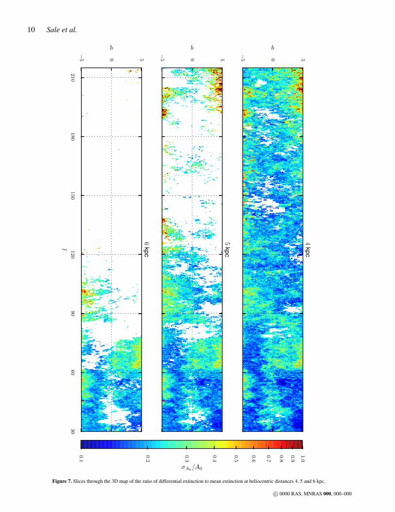
Figures 6 and 7 show the ratio of differential to mean extinc-tion. As well as being a nuisance factor, differential extinction isalso physically interesting: its extent is thought to be related to theMach number in the ISM (e.g Padoan, Jones & Nordlund 1997). Aswould be expected from theory (e.g. Lazarian & Pogosyan 2000;Fischera & Dopita 2004) and as a consequence of the outer scale ofISM turbulence being short relative to the length of our sightline,we find that the ratio of differential to mean extinction drops withincreasing distance. We also find that the strength of differential ex-tinction is significantly greater than the uncertainties on the meanextinction. Therefore, although we can state the value of mean ex-tinction within each voxel of the extinction map to high precision,we are unable to give an estimate of the extinction to a particularposition within the voxel as precisely. This has significant impactin applications such as the use of distance-extinction relationshipsto estimate a distance to an object of known extinction: indeed, inthese applications the uncertainty will be dominated by differentialextinction.

We also note that the measured differential extinctions dependon the size of the angular resolution element. As dust density iscorrelated over distances up to ∼ 100 pc, it follows that measuredextinctions for two given directions will also be correlated, with thecorrelation dropping with increasing angular separation. As a resultdifferential extinction will be greater when the angular resolutionelement is larger. Accordingly, we must stress that the measureddifferential extinctions are specific to the gridding of angular reso-lution elements employed here.

In Appendix A we describe the form the extinction map takes

c© 0000 RAS, MNRAS 000, 000–000

A 3D extinction map of the Northern Galactic Plane 9

−5 0 5

b

1kpc

−5 0 5

b

2kpc

30

60

90

120

150

180

210

l

−5 0 5

b

3kpc

0.1

0.2

0.3

0.4

0.5

0.6

0.7

0.8

0.9

1.0

σA0/A0

Figure 6. Slices through the 3D map of the ratio of differential extinction to mean extinction at heliocentric distances of 1, 2 and 3 kpc.

c© 0000 RAS, MNRAS 000, 000–000

10 Sale et al.

−5 0 5

b

4kpc

−5 0 5

b

5kpc

30

60

90

120

150

180

210

l

−5 0 5

b

6kpc

0.1

0.2

0.3

0.4

0.5

0.6

0.7

0.8

0.9

1.0

σA0/A0

Figure 7. Slices through the 3D map of the ratio of differential extinction to mean extinction at heliocentric distances 4, 5 and 6 kpc.

c© 0000 RAS, MNRAS 000, 000–000

A 3D extinction map of the Northern Galactic Plane 11

0.00

0.05

0.10

0.15

0.20

0.25

0.00

0.05

0.10

0.15

0.20

0.25

N/N

TO

TA

L

1 10 30

A0/AM06Ks

0.00

0.05

0.10

0.15

0.20

0.25

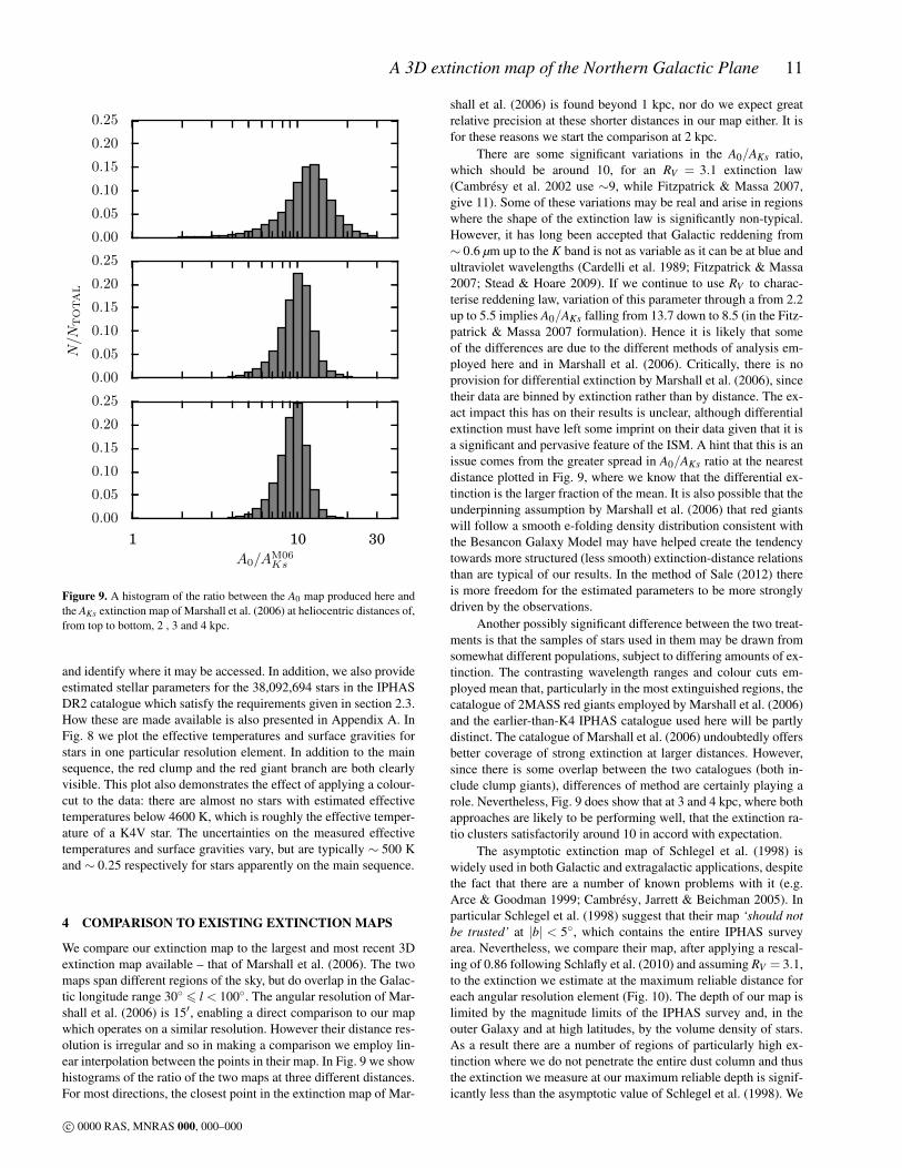
Figure 9. A histogram of the ratio between the A0 map produced here andthe AKs extinction map of Marshall et al. (2006) at heliocentric distances of,from top to bottom, 2 , 3 and 4 kpc.

and identify where it may be accessed. In addition, we also provideestimated stellar parameters for the 38,092,694 stars in the IPHASDR2 catalogue which satisfy the requirements given in section 2.3.How these are made available is also presented in Appendix A. InFig. 8 we plot the effective temperatures and surface gravities forstars in one particular resolution element. In addition to the mainsequence, the red clump and the red giant branch are both clearlyvisible. This plot also demonstrates the effect of applying a colour-cut to the data: there are almost no stars with estimated effectivetemperatures below 4600 K, which is roughly the effective temper-ature of a K4V star. The uncertainties on the measured effectivetemperatures and surface gravities vary, but are typically ∼ 500 Kand ∼ 0.25 respectively for stars apparently on the main sequence.

4 COMPARISON TO EXISTING EXTINCTION MAPS

We compare our extinction map to the largest and most recent 3Dextinction map available – that of Marshall et al. (2006). The twomaps span different regions of the sky, but do overlap in the Galac-tic longitude range 30◦ 6 l < 100◦. The angular resolution of Mar-shall et al. (2006) is 15′, enabling a direct comparison to our mapwhich operates on a similar resolution. However their distance res-olution is irregular and so in making a comparison we employ lin-ear interpolation between the points in their map. In Fig. 9 we showhistograms of the ratio of the two maps at three different distances.For most directions, the closest point in the extinction map of Mar-

shall et al. (2006) is found beyond 1 kpc, nor do we expect greatrelative precision at these shorter distances in our map either. It isfor these reasons we start the comparison at 2 kpc.

There are some significant variations in the A0/AKs ratio,which should be around 10, for an RV = 3.1 extinction law(Cambresy et al. 2002 use ∼9, while Fitzpatrick & Massa 2007,give 11). Some of these variations may be real and arise in regionswhere the shape of the extinction law is significantly non-typical.However, it has long been accepted that Galactic reddening from∼ 0.6 µm up to the K band is not as variable as it can be at blue andultraviolet wavelengths (Cardelli et al. 1989; Fitzpatrick & Massa2007; Stead & Hoare 2009). If we continue to use RV to charac-terise reddening law, variation of this parameter through a from 2.2up to 5.5 implies A0/AKs falling from 13.7 down to 8.5 (in the Fitz-patrick & Massa 2007 formulation). Hence it is likely that someof the differences are due to the different methods of analysis em-ployed here and in Marshall et al. (2006). Critically, there is noprovision for differential extinction by Marshall et al. (2006), sincetheir data are binned by extinction rather than by distance. The ex-act impact this has on their results is unclear, although differentialextinction must have left some imprint on their data given that it isa significant and pervasive feature of the ISM. A hint that this is anissue comes from the greater spread in A0/AKs ratio at the nearestdistance plotted in Fig. 9, where we know that the differential ex-tinction is the larger fraction of the mean. It is also possible that theunderpinning assumption by Marshall et al. (2006) that red giantswill follow a smooth e-folding density distribution consistent withthe Besancon Galaxy Model may have helped create the tendencytowards more structured (less smooth) extinction-distance relationsthan are typical of our results. In the method of Sale (2012) thereis more freedom for the estimated parameters to be more stronglydriven by the observations.

Another possibly significant difference between the two treat-ments is that the samples of stars used in them may be drawn fromsomewhat different populations, subject to differing amounts of ex-tinction. The contrasting wavelength ranges and colour cuts em-ployed mean that, particularly in the most extinguished regions, thecatalogue of 2MASS red giants employed by Marshall et al. (2006)and the earlier-than-K4 IPHAS catalogue used here will be partlydistinct. The catalogue of Marshall et al. (2006) undoubtedly offersbetter coverage of strong extinction at larger distances. However,since there is some overlap between the two catalogues (both in-clude clump giants), differences of method are certainly playing arole. Nevertheless, Fig. 9 does show that at 3 and 4 kpc, where bothapproaches are likely to be performing well, that the extinction ra-tio clusters satisfactorily around 10 in accord with expectation.

The asymptotic extinction map of Schlegel et al. (1998) iswidely used in both Galactic and extragalactic applications, despitethe fact that there are a number of known problems with it (e.g.Arce & Goodman 1999; Cambresy, Jarrett & Beichman 2005). Inparticular Schlegel et al. (1998) suggest that their map ‘should notbe trusted’ at |b| < 5◦, which contains the entire IPHAS surveyarea. Nevertheless, we compare their map, after applying a rescal-ing of 0.86 following Schlafly et al. (2010) and assuming RV = 3.1,to the extinction we estimate at the maximum reliable distance foreach angular resolution element (Fig. 10). The depth of our map islimited by the magnitude limits of the IPHAS survey and, in theouter Galaxy and at high latitudes, by the volume density of stars.As a result there are a number of regions of particularly high ex-tinction where we do not penetrate the entire dust column and thusthe extinction we measure at our maximum reliable depth is signif-icantly less than the asymptotic value of Schlegel et al. (1998). We

c© 0000 RAS, MNRAS 000, 000–000

12 Sale et al.

3060

90120

150180

210

l

−5 0 5

b

0.5

1.0

2.0

Amax0 /ASFD

V

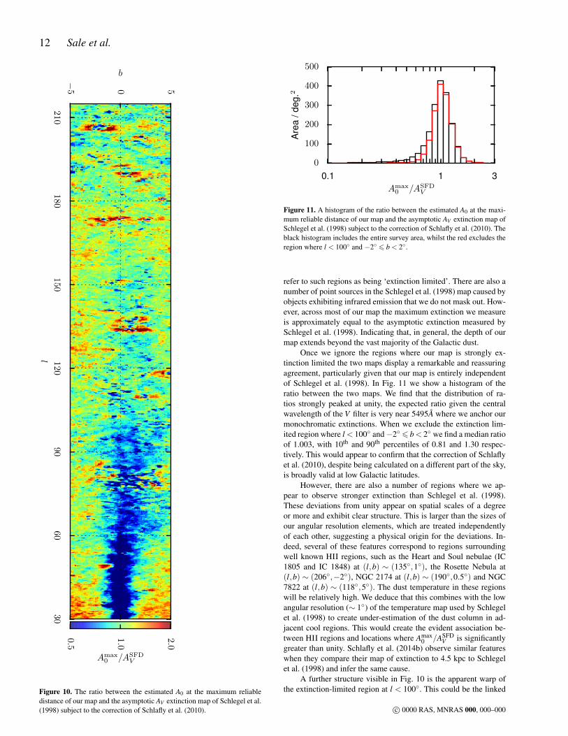
Figure 10. The ratio between the estimated A0 at the maximum reliabledistance of our map and the asymptotic AV extinction map of Schlegel et al.(1998) subject to the correction of Schlafly et al. (2010).

0.1 1 3Amax

0 /ASFDV

0

100

200

300

400

500

Are

a/d

eg.2

Figure 11. A histogram of the ratio between the estimated A0 at the maxi-mum reliable distance of our map and the asymptotic AV extinction map ofSchlegel et al. (1998) subject to the correction of Schlafly et al. (2010). Theblack histogram includes the entire survey area, whilst the red excludes theregion where l < 100◦ and −2◦ 6 b < 2◦.

refer to such regions as being ‘extinction limited’. There are also anumber of point sources in the Schlegel et al. (1998) map caused byobjects exhibiting infrared emission that we do not mask out. How-ever, across most of our map the maximum extinction we measureis approximately equal to the asymptotic extinction measured bySchlegel et al. (1998). Indicating that, in general, the depth of ourmap extends beyond the vast majority of the Galactic dust.

Once we ignore the regions where our map is strongly ex-tinction limited the two maps display a remarkable and reassuringagreement, particularly given that our map is entirely independentof Schlegel et al. (1998). In Fig. 11 we show a histogram of theratio between the two maps. We find that the distribution of ra-tios strongly peaked at unity, the expected ratio given the centralwavelength of the V filter is very near 5495A where we anchor ourmonochromatic extinctions. When we exclude the extinction lim-ited region where l < 100◦ and−2◦6 b< 2◦ we find a median ratioof 1.003, with 10th and 90th percentiles of 0.81 and 1.30 respec-tively. This would appear to confirm that the correction of Schlaflyet al. (2010), despite being calculated on a different part of the sky,is broadly valid at low Galactic latitudes.

However, there are also a number of regions where we ap-pear to observe stronger extinction than Schlegel et al. (1998).These deviations from unity appear on spatial scales of a degreeor more and exhibit clear structure. This is larger than the sizes ofour angular resolution elements, which are treated independentlyof each other, suggesting a physical origin for the deviations. In-deed, several of these features correspond to regions surroundingwell known HII regions, such as the Heart and Soul nebulae (IC1805 and IC 1848) at (l,b) ∼ (135◦,1◦), the Rosette Nebula at(l,b) ∼ (206◦,−2◦), NGC 2174 at (l,b) ∼ (190◦,0.5◦) and NGC7822 at (l,b) ∼ (118◦,5◦). The dust temperature in these regionswill be relatively high. We deduce that this combines with the lowangular resolution (∼ 1◦) of the temperature map used by Schlegelet al. (1998) to create under-estimation of the dust column in ad-jacent cool regions. This would create the evident association be-tween HII regions and locations where Amax

0 /ASFDV is significantly

greater than unity. Schlafly et al. (2014b) observe similar featureswhen they compare their map of extinction to 4.5 kpc to Schlegelet al. (1998) and infer the same cause.

A further structure visible in Fig. 10 is the apparent warp ofthe extinction-limited region at l < 100◦. This could be the linked

c© 0000 RAS, MNRAS 000, 000–000

A 3D extinction map of the Northern Galactic Plane 13

to warp in the Galactic dust disc that exists beyond the maximumdepth of our map (cf. Levine et al. 2006). In this region our maphas a depth of ∼ 5 kpc.

5 CLOSING DISCUSSION

We have presented a new three-dimensional extinction map of thenorthern Galactic Plane. The map is produced using the IPHASDR2 catalogue, which due to its filter set incorporating Hα is par-ticularly well suited to the task. Using these data we have been ableto produce a map with fine angular (typically 10 ′) and distance(100 pc) resolutions.

As well as the extinction map we also produce estimates ofthe distance, extinction, effective temperature, surface gravity, andmass for 38,092,694 stars. The maps and estimated stellar param-eters are both being made available on line at http://www.iphas.org/extinction.

In Fig. 5 there are a number of azimuthal discontinuities, or‘fingers of God’. Similar features are also visible in Fig 9 of Mar-shall et al. (2006). These features can only exist because both meth-ods treat different sightlines independently and are exaggerated bythe fact that measured extinction is strongly correlated betweenvoxels along a line of sight. However, we know that no part of theISM exists in isolation: dust density and thus extinction should becorrelated between nearby regions and and it would be preferredthat methods for mapping extinction would account for this corre-lation.

We find that the main source of uncertainty in extinction to agiven position arises from differential extinction, rather than fromuncertainty in the mean extinction. This has its origins in the fractalnature of the ISM. This is exacerbated by the way we bin the data:stars which are only a few arcseconds apart on the sky are treatedin the same way as those which are further apart, but still lie in thesame resolution element. This treatment runs contrary to our physi-cal intuition, that the extinction to closely separated stars should bemore tightly correlated than that to stars more distantly spread.

Sale & Magorrian (2014) presents a method which overcomesboth of these shortcomings by fitting a Gaussian random field tologA, building in a physical model of interstellar turbulence. In thisway, the closest stars to a point most heavily affect the estimatedvalue of extinction, whilst those further afield – potentially sev-eral degrees away – influence the estimated value of extinction toa lesser extent. This development should lead to extinction mapswithout unphysical discontinuities and permit more precise esti-mates of extinction to individual objects.

The strength of the produced extinction map rests to a largedegree on the IPHAS data employed. The inclusion of the narrow-band Hα filter essentially represents the cheapest conceivable spec-troscopy: the combination of it with the r filter allows the Hα

equivalent width to be directly estimated, offering a level of detailnot usually accessed by broadband photometry. A similar facilitywas available before via Stromgren uvbyHβ photometry. Howeverthe clear advantages of Hα are the penetration of longer sightlinesmade possible by its redder wavelength and its typically strongersignature.

The extinction map we produce is sensitive to zero-point er-rors in the data (Sale et al. 2009). The recently completed globalphotometric calibration of IPHAS has enabled us to produce a re-liable, internally-consistent extinction map. The comparisons wehave made indicate the extinction map is astrophysically credible,which in turn underwrites the quality of the IPHAS’ photometric

calibration. We can commend the use of the inferred extinctiontrends on spatial scales ranging from∼ 1 kpc up to 5-6 kpc for mostsightlines (see Fig. 2), noting that differential extinction moderatesas a source of uncertainty as distance rises. This spatial range com-plements that of the map of Lallement et al. (2014), which providesgood coverage out to 1 kpc.

The method of Sale (2012), which we employ here, is notbound to any particular photometric data set. Thus it would be pos-sible, in the future, to combine IPHAS data with data from othersurveys, such as UKIDSS-GPS (Lucas et al. 2008) in the near in-frared or UVEX (Groot et al. 2009), the ongoing blue counterpartto IPHAS. The VST/OmegaCam Photometric Hα Survey of theSouthern Galactic Plane and Bulge (VPHAS+; Drew et al. 2014),which commenced in late December 2011, is the southern part-ner of IPHAS, observing the other half of the Galactic Plane andthe Bulge. VPHAS+ also employs the r, i and Hα filters, alongwith the u and g filters. As the VPHAS+ filter set mirrors theIPHAS/UVEX filter set and the surveys share essentially the samestrategy, it should be straightforward, in due course, to apply re-finements to the current method to all three surveys combined inorder to complete an extinction map of the entire Galactic Plane.Looking further into the future, optical and near-infrared photome-try, including Hα, collected across a range of ground-based surveyscould be combined with Gaia parallaxes, as they become available,to produce much sharper, more compelling 3D maps of Galacticextinction.

ACKNOWLEDGEMENTS

The authors would like to thank John Magorrian, Christian Knigge,Antonio Mampaso, Quentin Parker and Albert Zijlstra for construc-tive comments and discussions.

SES, JED and GB acknowledge support from the UnitedKingdom Science Technology and Facilities Council (STFC, SESST/K00106X/1, JED and GB ST/J001333/1). HJF acknowledgesthe receipt of an STFC studentship. PRG is supported by a Ramony Cajal fellowship (RYC-2010-05762), and acknowledges supportprovided by the Spanish MINECO AYA2012-38700 grant. Theresearch leading to these results has received funding from theEuropean Research Council under the European Union’s SeventhFramework Programme (FP/2007-2013) / ERC Grant Agreementn. 320964 (WDTracer).

This paper makes use of data obtained as part of the INT Pho-tometric Hα Survey of the Northern Galactic Plane (IPHAS) car-ried out at the Isaac Newton Telescope (INT). The INT is operatedon the island of La Palma by the Isaac Newton Group in the Span-ish Observatorio del Roque de los Muchachos of the Instituto deAstrofısica de Canarias.

REFERENCES

Arce H. G., Goodman A. A., 1999, ApJ, 512, L135Arenou F., Grenon M., Gomez A., 1992, A&A, 258, 104Bailer-Jones C. A. L., 2011, MNRAS, 411, 435Barentsen G. et al., 2014, preprint (arXiv:1406.4862)Berry M. et al., 2012, ApJ, 757, 166Bressan A., Marigo P., Girardi L., Salasnich B., Dal Cero C., Rubele S.,

Nanni A., 2012, MNRAS, 427, 127Cambresy L., Beichman C. A., Jarrett T. H., Cutri R. M., 2002, AJ, 123,

2559Cambresy L., Jarrett T. H., Beichman C. A., 2005, A&A, 435, 131

c© 0000 RAS, MNRAS 000, 000–000

14 Sale et al.

Cardelli J. A., Clayton G. C., Mathis J. S., 1989, ApJ, 345, 245Chepurnov A., Lazarian A., 2010, ApJ, 710, 853Drew J. E. et al., 2005, MNRAS, 362, 753Drew J. E. et al., 2014, MNRAS, 440, 2036Fischera J., Dopita M. A., 2004, ApJ, 611, 919Fitzpatrick E. L., Massa D., 2007, ApJ, 663, 320Gonzalez-Solares E. A. et al., 2008, MNRAS, 388, 89Green G. M. et al., 2014, ApJ, 783, 114Groot P. J. et al., 2009, MNRAS, 1184Jahreiß H., Wielen R., 1997, in R.M. Bonnet, E. Høg, P.L. Bernacca,

L. Emiliani, A. Blaauw, C. Turon, J. Kovalevsky, L. Lindegren, H. Has-san, M. Bouffard, B. Strim, D. Heger, M.A.C. Perryman, L. Woltjer, eds,Hipparcos - Venice ’97. ESA Special Publication, Vol. 402, pp. 675–680

Juric M. et al., 2008, ApJ, 673, 864Lallement R., Vergely J. L., Valette B., Puspitarini L., Eyer L., Casagrande

L., 2014, A&A, 561, A91Lazarian A., Pogosyan D., 2000, ApJ, 537, 720Levine E. S., Blitz L., Heiles C., 2006, ApJ, 643, 881Loredo T. J., 2004, in R. Fischer, R. Preuss, U.V. Toussaint, eds, Ameri-

can Institute of Physics Conference Series. American Institute of PhysicsConference Series, Vol. 735, pp. 195–206

Lucas P. W. et al., 2008, MNRAS, 391, 136Majewski S. R., Zasowski G., Nidever D. L., 2011, ApJ, 739, 25Marshall D. J., Robin A. C., Reyle C., Schultheis M., Picaud S., 2006,

A&A, 453, 635Neckel T., Klare G., 1980, A&AS, 42, 251Padoan P., Jones B. J. T., Nordlund A. P., 1997, ApJ, 474, 730Planck Collaboration et al., 2013, preprint (arXiv:1312.1300)Reid M. J. et al., 2014, ApJ, 783, 130Roberts G. O., Rosenthal J. S., 2001, Statistical science, 16, 351Roberts G. O., Rosenthal J. S., 2009, Journal of Computational and Graph-

ical Statistics, 18, 349Sale S. E., 2012, MNRAS, 427, 2119Sale S. E., Magorrian J., 2014, preprint (arXiv:1406.1177)Sale S. E. et al., 2009, MNRAS, 392, 497Schlafly E. F., Finkbeiner D. P., Schlegel D. J., Juric M., Ivezic Z., Gibson

R. R., Knapp G. R., Weaver B. A., 2010, ApJ, 725, 1175Schlafly E. F. et al., 2014a, ApJ, 786, 29Schlafly E. F. et al., 2014b, preprint (arXiv:1405.2922)Schlegel D. J., Finkbeiner D. P., Davis M., 1998, ApJ, 500, 525Spangler S. R., Gwinn C. R., 1990, ApJ, 353, L29Stead J. J., Hoare M. G., 2009, MNRAS, 400, 731Tarantola A., Valette B., 1982, Reviews of Geophysics and Space Physics,

20, 219Tierney L., 1994, Annals of Statistics, 22, 1701Trumpler R. J., 1930, PASP, 42, 214Vallee J. P., 2013, International Journal of Astronomy and Astrophysics,

3, 20Vergely J. L., Valette B., Lallement R., Raimond S., 2010, A&A, 518, A31

APPENDIX A:

A1 The extinction map

Both the 3D extinction map and the catalogue of stellar parametersare available at http://www.iphas.org/extinction andwill also be made available via the CDS.

The extinction map is presented in two forms. First, we pub-lish the posterior expectations of mean extinction and differentialextinction for every voxel in the map. These expectations are ac-companied by measurements of the half-widths of 68.3 per centcredible intervals centred on the expectation for both mean extinc-tion and differential extinction. In addition we also make available20 samples from the posterior distribution on the mean extinction.

For each angular resolution element the maximum reliabledistance is also provided. Measurements of mean extinction and

other parameters for the voxels beyond the maximum reliable dis-tance are published, but for reference purposes only. These datapoints depend very heavily on the assumed priors and are not soheavily constrained by data in the IPHAS DR2 catalogue – conse-quently, they should not be relied upon.

A2 Stellar parameters

Estimated stellar parameters for the 38,092,694 stars in the stud-ied catalogue are also made available. In particular, we publishestimates of the distance, extinction, effective temperature, sur-face gravity, and mass for each of these stars. For each parame-ter we provide the mean and standard deviation of the correspond-ing marginal posterior distribution. The coordinates of each starare also included so as to facilitate cross-matching with the mainIPHAS DR2 catalogue of Barentsen et al. (2014). An extract fromthis catalogue is shown in Table A1.

By publishing only expectations and one dimensional standarddeviations we are passing on only a relatively crude depiction ofthe posterior probability distribution. Consequently features suchas multimodality of the posterior and covariance between parame-ters will not be apparent. Additionally, the calculation of the stellarparameters has been subject to both a set of priors and a surveyselection function, both of which have heavily shaped the resultsobtained. Any further analysis of these data will also be inevitablysubject to these same priors and selection function. In light of thesefactors, we caution the reader that great care must be taken not toover-interpret or mistake patterns which appear in this catalogue.These data are provided in the spirit that they may be a useful re-source for e.g. target selection for spectroscopic programmes or forthe interested reader to gain insight into the origin of features in theextinction map.

APPENDIX B: MAPS OF UNCERTAINTY

c© 0000 RAS, MNRAS 000, 000–000

A 3D extinction map of the Northern Galactic Plane 15

−5 0 5

b

1kpc

−5 0 5

b

2kpc

30

60

90

120

150

180

210

l

−5 0 5

b

3kpc

0.0

1

0.0

2

0.0

3

0.0

4

0.0

5

0.0

6

0.0

7

0.0

8

0.0

9

0.1

0

dA0/A0

Figure B1. Slices through the 3D map of relative uncertainty on mean extinction at heliocentric distances of 1, 2 and 3 kpc.

c© 0000 RAS, MNRAS 000, 000–000

16 Sale et al.

−5 0 5

b

4kpc

−5 0 5

b

5kpc

30

60

90

120

150

180

210

l

−5 0 5

b

6kpc

0.0

1

0.0

2

0.0

3

0.0

4

0.0

5

0.0

6

0.0

7

0.0

8

0.0

9

0.1

0

dA0/A0

Figure B2. Slices through the 3D map of relative uncertainty on mean extinction at heliocentric distances of 4, 5 and 6 kpc.

c© 0000 RAS, MNRAS 000, 000–000

A 3D extinction map of the Northern Galactic Plane 17

Name l/◦ b/◦ s/ pc ds/ pc A0 dA0 log(Teff/K) d log(Teff/K) logg d logg M/M� dM/M�

IPHAS2 J190008.19-042400.0 30.00006 -3.9367 4965 1481 1.60 0.25 3.782 0.033 4.41 0.15 1.02 0.16IPHAS2 J190009.37-042408.9 30.00009 -3.94219 6149 2222 2.09 0.49 3.793 0.059 4.36 0.17 1.17 0.26IPHAS2 J190018.64-042519.3 30.00011 -3.98536 4305 1086 1.45 0.22 3.767 0.029 4.43 0.12 1.03 0.14IPHAS2 J190021.28-042539.2 30.00014 -3.99767 5800 1691 1.84 0.33 3.785 0.039 4.37 0.14 1.10 0.19IPHAS2 J190015.86-042458.0 30.00015 -3.97239 3972 1282 1.36 0.21 3.763 0.029 4.38 0.17 1.03 0.14IPHAS2 J190020.90-042535.5 30.00034 -3.99578 4573 1650 1.66 0.27 3.787 0.035 4.34 0.19 1.09 0.19IPHAS2 J190006.36-042344.8 30.00038 -3.928 8521 1791 2.75 0.32 3.725 0.041 3.40 0.21 1.32 0.21IPHAS2 J190008.65-042402.1 30.00042 -3.93867 1024 224 1.10 0.18 3.722 0.024 4.55 0.09 0.85 0.07IPHAS2 J190010.71-042416.5 30.00074 -3.9481 1792 376 1.18 0.19 3.731 0.027 4.53 0.08 0.88 0.09IPHAS2 J190016.67-042501.1 30.0009 -3.97578 2771 1363 1.36 0.26 3.739 0.034 4.43 0.23 0.91 0.15IPHAS2 J190004.32-042326.9 30.00099 -3.9182 1828 824 1.17 0.17 3.746 0.025 4.35 0.25 0.99 0.13

Table A1. An extract from the catalogue of stellar parameters, where s represents the distance to the stars. The full catalogue is available online via http://www.iphas.org/extinction

c© 0000 RAS, MNRAS 000, 000–000