9781461467168-c1.pdf

Chapter 2

Measuring Instruments and Their Properties

2.1 Types of Measuring Instruments

Measuring instruments are the technical objects that are specially developed for

the purpose of measuring specific quantities. A general property of measuring

instruments is that their accuracy is known. Measuring instruments are divided

into material measures, measuring transducers, indicating instruments, recording

instruments, and measuring systems.

A material measure is a measuring instrument that reproduces one or more

known values of a given quantity. Examples of measures are balance weights,

measuring resistors, measuring capacitors, and reference materials. Single-valued

measures, multiple-valued measures, and collections of measures are distinguished.

Examples of multiple-valued measures are graduated rulers, measuring tapes,

resistance boxes, and so on. Multiple-valued measures are further divided into

those that reproduce discrete values of the corresponding quantities, such as

resistance boxes, and those that continuously reproduce quantities in some range,

for example, a measuring capacitor with variable capacitance. Continuous

measures are usually less accurate than discrete measures.

When measures are used to perform measurements, the measurands are com-

pared with the known quantities reproduced by the measures. The comparison is

made by different methods, but so-called comparators are a specific means that are

used to compare quantities. A comparator is a measuring device that makes it

possible to compare similar quantities and has a known sensitivity. The simplest

comparator is the standard equal-armed pan balance.

In some cases, quantities are compared without comparators, by experimenters,

with the help of their viewing or listening perceptions. For instance, when measur-

ing the length of a body with the help of a ruler, the ruler is placed on the body and

the observer fixes visually the graduations of the ruler (or fractions of a graduation)

at the corresponding points of the body.

S.G. Rabinovich, Evaluating Measurement Accuracy: A Practical Approach,DOI 10.1007/978-1-4614-6717-5_2, # Springer Science+Business Media New York 2013

31

A measuring transducer is a measuring instrument that converts the measurement

signals into a form suitable for transmission, processing, or storage. Themeasurement

information at the output of a measuring transducer typically cannot be directly

observed by the experimenter.

One must distinguish measuring transducers and the transforming elements of

a complicated instrument. The former are measuring instruments, and as such, they

have rated (i.e., listed in documentation) metrological properties (see below). The

latter, on the other hand, do not have an independent metrological significance and

cannot be used separately from the instrument of which they are a part.

Measuring transducers are diverse. Thermocouples, resistance thermometers,

measuring shunts, and the measuring electrodes of pH meters are just a few

examples of measuring transducers. Measuring current or voltage transformers

and measuring amplifiers are also measuring transducers. This group of transducers

is characterized by the fact that the signals at their inputs and outputs are a quantity

of the same kind, and only the magnitude of the quantity changes. For this reason,

these measuring transducers are called scaling measuring transducers.Measuring transducers that convert an analog signal at the input into a discrete

signal at the output are called analog-to-digital converters. Such converters are

manufactured either as autonomous, i.e., independent measuring instruments, or as

units built into other instruments, in particular, in the form of integrated

microcircuits. Analog-to-digital converters are a necessary component of a variety

of digital devices, but they are also employed in monitoring, regulating, and control

systems.

An indicating instrument is a measuring instrument that is used to convert

measurement signals into a form that can be directly perceived by the observer.

Based on the design of the input circuits, indicating instruments are just as diverse

as measuring transducers, and it is difficult to survey all of them. Moreover, such a

review and even classification are more important for designing instruments than

for describing their general properties.

A common feature of all indicating instruments is that they all have readout

devices. If these devices are implemented in the form of a scale and an indicating

needle, then the indications of the instrument are a continuous function of the

magnitude of the measurable quantity. Such instruments are called analog

instruments. If the indications of instruments are in a digital form, then such

instruments are called digital instruments.

The above definition of digital instruments formally includes two types of

devices. The first type, which includes automatic digital voltmeters, bridges, and

similar instruments, performs all measuring transformations in a discrete form; in

the second type, exemplified by induction meters for measuring electrical energy,

all measuring transformations of signals occur in an analog form and only the

output signal assumes a discrete form. The conversions of measurement informa-

tion into a discrete form have several specific features. Therefore, only instruments

in which the measurement conversions occur in a discrete form are usually consid-

ered to be digital instruments.

32 2 Measuring Instruments and Their Properties

The indications of digital instruments can be easily recorded and are convenient

for entering into a computer. In addition, their design usually makes it possible to

obtain significantly higher accuracy than the accuracy of analog instruments.

Moreover, when digital instruments are employed, no reading errors occur. How-

ever, with analog instruments, it is easier to judge trends in the variation of the

measurands.

In addition to analog and digital instruments, there also exist analog-discrete

measuring instruments. In these instruments, the measuring conversions are

performed in an analog form, but the readout means are discrete (but not digital).

Analog-discrete instruments combine the advantages of both analog and digital

instruments. Mentioned above induction meters for measuring electric energy are

examples of such hybrid instruments.

In many cases, measuring instruments are designed to record their indications.

Such instruments are called recording instruments. Data can be recorded in the

form of a continuous record of the variation of the measurand in time, or in the form

of a series of discrete points. Instruments of the first type are called automatic-

plotting instruments, and instruments of the second type are called printing

instruments. Printing instruments can record the values of a measurand in digital

form. Printing instruments give a discrete series of values of the measurand with

some time interval. The continuous record provided by automatic-plotting

instruments can be regarded as an infinite series of values of the measurand.

Sometimes measuring instruments are equipped with induction, photo-optical,

or contact devices and relays for purposes of control or regulation. Such instruments

are called regulating instruments. Regulating units typically lead to some reduction

of the accuracy of the measuring instrument.

Measuring instruments also customarily include null indicators, whose primary

purpose is to detect the presence of a nonzero signal. The reason for them to be

considered measuring instruments is that a null indicator, such as a galvanometer,

can often be used as a highly sensitive indicating instrument.

A measuring system is a collection of functionally integrated measuring, com-

puting, and auxiliary devices connected to each other with communication

channels.

2.2 Metrological Characteristics of Measuring Instruments

We shall divide all characteristics of measuring instruments into two groups:

metrological, which are significant for using a measuring instrument in the manner

intended, and secondary. We shall include in the latter such characteristics as mass,

dimensions, and degree of protection from moisture and dust. We shall not discuss

secondary characteristics because they are not directly related with the measure-

ment accuracy, even though they sometimes influence the selection and application

of an instrument.

2.2 Metrological Characteristics of Measuring Instruments 33

By metrological characteristics of a measuring instrument, we mean the

characteristics that make it possible to judge the suitability of the instrument for

performing measurements in a known range with known accuracy. A simple

example of a metrological characteristic common to all measuring instruments

except single measures (i.e., measures reproducing a single value of a quantity) is

the measurement range of the instrument. We will call metrological characteristics

that are established before or during the design and development of the instrument

as nominal metrological characteristics. Examples of such a characteristic are the

nominal value of a measure (10 Ω, 1 kG, etc.), the measurement range of an

instrument (0–300V, 0–1,200�C, etc.), the conversion range of a transducer, the

value of the scale factor of an instrument scale, and so on.

The relation between the input and the output signals of indicating instruments and

transducers is determined by the transfer function. For indicating instruments, this

relation is determined by the instrument scale, whereas for measuring transducers, it is

determined by a graph or an equation. If this graph or equation had been determined

and specified before the transducer was developed (or during its development), then

the graph or equation represents a nominal metrological characteristic.

The real characteristics of measuring instruments differ from the nominal

characteristics because of fabrication inaccuracies and changes occurring in the

corresponding properties in time. These differences between nominal and real

metrological characteristics lead to the error of the instrument.

Ideally, a measuring instrument would react only to the measured quantity or to

the parameter of the input signal of interest, and its indication would not depend on

the external conditions, such as the power supply regime, temperature, and so on. In

reality, the external conditions do affect the indications of the instrument. The

quantities characterizing the external conditions affecting the indications of a

measuring instrument are called influence quantities.For some types of measuring instruments, the dependence of the output signal or

the indications on a given influence quantity can be represented as a functional

dependence, called the influence function. The influence function can be expressed

in the form of an equation (e.g., the temperature dependence of the EMF of standard

cells) or a graph. In the case of a linear dependence, it is sufficient to give the

coefficient of proportionality between the output quantity and the influence quan-

tity. We call this coefficient the influence coefficient. Influence coefficients and

functions make it possible to take into account the conditions under which measur-

ing instruments are used, by introducing the corresponding corrections to the

obtained results.

The imperfection of measuring instruments is also manifested because when the

same quantity is measured repeatedly under identical conditions, the results can

differ somewhat from one another. If these differences are significant, the

indications are said to be nonrepeatable.

The inaccuracy of a measuring instrument is usually characterized by its error.

Taking an indicating instrument as an example, let the true value of a quantity at the

input of the instrument be At and the instrument indication be the value Ar. The

absolute error of the instrument will be


ζ ¼ Ar � At:

If the indications of the repeated measurements of At are somewhat different,

(but not enough to be considered nonrepeatable), one can talk about a random

component of instrument error. For analog instruments, the random component of

instrument error is normally caused by friction in the supports of a movable part of

the instrument and/or by hysteresis phenomena. The limits of this error component

can be found directly if the quantity measured by the instrument can be varied

continuously, which is the case with, e.g., the electric current or voltage. The

common method involves driving the indicator of the instrument continuously up

to the same scale marker, once from below and once from above the marker.

To compensate for friction (and/or hysteresis), the input signal that drives the

indicator to the marker from below needs to be higher than what it would have

been without friction; the input signal that drives the indicator to the same marker

from above will be smaller. We will call the dead band the absolute value of the

difference between the two values of the measurand that are obtained in such a test

corresponding to a given scale marker of the instrument. The dead band gives the

range of possible values of the random component of instrument error, and one half

of this length is the limiting value of the random error.

There are also several instrument types, notably, weighing scales, whose

indications cannot vary continuously. The random error of weighing scales is

usually characterized by the standard deviation [7]. This characteristic of an

instrument is calculated from the changes produced in the indications of the scales

by a load with a known mass; the test is performed at several scale markers,

including the limits of the measurement range. One method for performing the

tests and the computational formula for calculating the standard deviation of

weighing scales are presented in [7].

Measuring instruments are created to bring certainty into the phenomena studied

and to establish regular relations between the phenomena. Thus, the uncertainty

created by the nonrepeatability of instrument indications interferes with using an

instrument in the manner intended. For this reason, the first problem that must be

solved when developing a new measuring device is to make its random error

insignificant, i.e., either negligibly small compared with other errors or falling

within permissible limits of error for measuring devices of the given type. We

should note here that because uncertainty of instrument indications represents only

a random component of its inaccuracy, the term “uncertainty” cannot replace the

term “limits of error” as applied to measuring instruments.

If the random error is insignificant and the elements determining instrument

accuracy are stable, then by calibration, the measuring device can always be “tied”

to a corresponding measurement standard and the potential accuracy of the instru-

ment can be realized.

The value of the measurand corresponding to the interval between two neighboring

markers on the instrument scale is called the value of a scale division. Similarly, the

value of the least significant digit is the value of the measurand corresponding to one

increment of the least significant digit of a digital readout device.

2.2 Metrological Characteristics of Measuring Instruments 35

The sensitivity of a measuring instrument is the ratio of the change in the output

value of the measuring instrument to the corresponding change in the input value of

the quantity that causes the output value to change. The sensitivity can be a nominal

metrological characteristic or an actual characteristic of a real instrument.

The discrimination threshold is the minimum change in the input signal that

causes an appreciable change in the output signal.

The resolution is the smallest interval between two distinguishable neighboring

discrete values of the output signal.

Instability (of a measuring instrument) is a general term that expresses the

change in any property of the measuring instrument in time.

Drift is the change occurring in the output signal (always in the same direction)

in the absence of the input signal over a period of time that is significantly longer

than the time needed to perform a measurement with a given measuring instrument.

The presence of drift entails the need to reset the zero indication of the instrument.

The drift and the instability do not depend on the input signal, but they can

depend on the external conditions. The drift is usually determined in the absence of

the signal at the input.

The metrological characteristics of measuring instruments should also include

their dynamic characteristics. These characteristics reflect the inertial properties of

measuring instruments. It is necessary to know them to correctly choose and use

many types of measuring instruments. The dynamical characteristics are examined

below in Sect. 2.5.

The properties of measuring instruments can normally be described based on the

characteristics enumerated above. For specific types of measuring instruments,

however, additional characteristics are often required. Thus, for the gauge rods,

the flatness and degree of polish are important. For voltmeters, the input resistance

is important. We shall not study such characteristics, because they refer only to

individual types of measuring instruments.

2.3 Rating of the Errors of Measuring Instruments

Measuring instruments can only be used as intended when their metrological

properties are known. In principle, the metrological properties can be established

by two methods. One method is to find the actual characteristics of a specific

instrument. In the second method, the nominal metrological characteristics and

the permissible deviations of the real characteristics from the nominal characteristics

are given.

The first method is laborious, and for this reason, it is used primarily for the most

accurate and stable measuring instruments. Thus, the second method is the main

method. The nominal characteristics and the permissible deviations from them are

given in the technical documentation when measuring instruments are designed,

which predetermines the properties of measuring instruments and ensures that they

are interchangeable.


In the process of using measuring instruments, their real properties are checked

to determine whether these properties deviate from the established nominal

characteristics. If some real property deviates from its nominal value by an amount

more than allowed, then the measuring instrument is adjusted, refurbished, or

discarded and no longer used.

Thus, the choice of the nominal characteristics of measuring instruments and the

designation of permissible deviations of the real characteristics from them – rating of

the metrological characteristics of measuring instruments – are of great importance

for measurement practice. The practice of rating the metrological characteristics of

measuring instruments has evolved over time, and we will examine it next.

Both the production of measuring instruments and the rating of their

characteristics initially arose spontaneously in each country. Later, rules that

brought order to the rating process were established in all countries with significant

instrument production. The recommendations developed at this time by interna-

tional organizations, primarily Publication 51 of the International Electrotechnical

Commission (IEC) and a number of publications by the International Organization

of Legal Metrology (OIML), were of great importance for standardizing the

expression of rated characteristics [8, 9]. The terminological documents are also

extremely valuable for developing rating procedures [1, 10, 12].

We shall now return to the gist of the problem. The values of nominal metrolog-

ical characteristics, such as the upper limits of measurement ranges, the nominal

values of the measures, the scale factors of instruments and so on, are chosen from a

standardized series of values of these characteristics. A more difficult task is to rate

the accuracy characteristics: errors and instability.

Despite the efforts of designers, the real characteristics of measuring instruments

depend to some extent on the external conditions. For this reason, the conditions are

determined under which the measuring instruments are to be calibrated and

checked, including the nominal values of all influence quantities and the ranges

of their permissible deviation from the nominal values. These conditions are called

reference conditions. The error of measuring instruments under reference

conditions is called the intrinsic error.In addition to the reference conditions and intrinsic errors, the rated operating

conditions of measuring instruments are also established, i.e., the conditions under

which the characteristics of measuring instruments remain within certain limits and

the measuring instruments can be employed as intended. Understandably, errors in

the rated operating conditions are larger than errors under the reference conditions.

This change is characterized by specifying the limits of the additional error(the additional error the instrument can have due to deviation of the corresponding

influence quantity from the reference condition), the permissible value of the

corresponding influence quantity, or by indicating the limits of the permissible

error under the rated operating conditions (the overall possible error of the

instrument).

The errors of measuring instruments are expressed not only in the form of

absolute and relative errors, adopted for estimating measurement errors, but also

in the form of fiducial errors. The fiducial error is the ratio of the permissible limits

2.3 Rating of the Errors of Measuring Instruments 37

of the absolute error of the measuring instrument to some standardized value –

fiducial value. The latter value is established by standards on separate types of

measuring instruments; we discuss these rules later in this section. The fiducial

error is somewhat similar to relative error but, since it is normalized to a constant

standardized value, the fiducial error is constant across the entire measurement

range of the device. The purpose of fiducial errors is that they make it possible to

compare the accuracy of measuring instruments that have different measurement

ranges. For example, the accuracy of an ammeter with a measurement limit of 1A

and permissible absolute error of 0.01A has the same fiducial error of 1% (and in

this sense, the same accuracy) as an ammeter with a measurement limit of 100A and

permissible absolute error of 1A.

For measuring transducers, the errors can be represented relative to either the

input or output signals. Let us consider the relationship between these two error

representations.

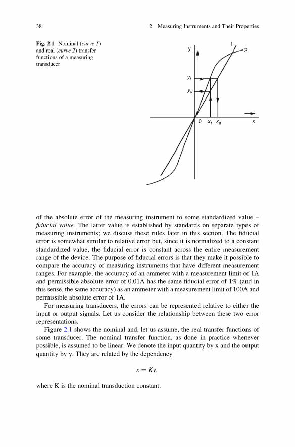
Figure 2.1 shows the nominal and, let us assume, the real transfer functions of

some transducer. The nominal transfer function, as done in practice whenever

possible, is assumed to be linear. We denote the input quantity by x and the output

quantity by y. They are related by the dependency

x ¼ Ky;

where K is the nominal transduction constant.

y

x0

12

xt xa

yt

ya

Fig. 2.1 Nominal (curve 1)and real (curve 2) transferfunctions of a measuring

transducer


At the point with true values of the quantities xt and yt, the true value of the

transduction constant will be Kt ¼ xt /yt. Calculations based on the nominal con-

stant K, however, result in an error.

Let xa ¼ Kyt and ya ¼ xt /K be determined based on yt and xt (see Fig. 2.1). Thenthe absolute transducer error with respect to the input will be

Δx ¼ xa � xt ¼ ðK � KtÞyt:

The error with respect to the output is expressed analogously:

Δy ¼ ya � yt ¼ 1

K� 1

Kt

� �xt:

We note, first, that Δx and Δy always have different signs: If (K – Kt) > 0, then

(1/K – 1/Kt) < 0.

But this is not the only difference. The quantities x and y can also have different

dimensions; i.e., they can be physically different quantities, so that the absolute

input and output errors are not comparable. For this reason, we shall study the

relative errors:

εx ¼ Δxxt

¼ ðK � KtÞ ytxt¼ K � Kt

Kt;

εy ¼ Δyyt

¼ ðKt � KÞKKt

xtyt¼ Kt � K

K:

As Kt 6¼ K, we have │εx│ 6¼ │εy│.We denote the relative error in the transduction constant at the point (xt ,yt) as εk,

where εk ¼ (K – Kt)/Kt. Then

εxεy

¼ �ð1þ εkÞ:

However, εk � 1, and in practice relative errors with respect to the input and

output can be regarded as equal in magnitude.

In measures, the rated error is determined as the difference between the nominal

value of the measure and the “true value” of the quantity reproduced by the

measure; the “true value” is obtained by another, known to be much more precise,

measurement. This is analogous to indicating instruments if one considers the

nominal value of a measure as the indication of the instrument.

It is interesting to note that single measures that reproduce passive quantities, for

example, mass, electric resistance, and so on, have only systematic errors. The error

of measures of active quantities (electric voltage, electric current, etc.) can have

both systematic and random components. Multiple-valued measures of passive

quantities can have random errors introduced by the switching elements.


To summarize, when the errors of measuring instruments are rated, the permissible

limits of the intrinsic and all additional errors are specified. At the same time, the

reference and rated operating conditions are indicated.

Of all forms enumerated above for expressing the errors of measuring

instruments, the best is the relative error, because in this case, the indication of

the permissible limit of error gives the clearest idea of the level of measurement

accuracy that can be achieved with the given measuring instrument. The relative

error, however, usually changes significantly over the measurement range of the

instrument, and for this reason, it is difficult to be rated.

The absolute error is frequently more convenient than the relative error. In the

case of an instrument with a scale, the limit of the permissible absolute error can be

rated with the same numerical value for the entire scale of the instrument. But then

it is difficult to compare the accuracies of instruments having different measure-

ment ranges. This difficulty disappears when the fiducial errors are rated.

Let us now consider how the limits of permissible errors are expressed. For our

discussion below, we shall follow primarily [9]. The limit of the permissible

absolute error can sometimes be expressed by a single value (neglecting the sign):

Δ ¼ �a;

sometimes in the form of the linear dependence:

Δ ¼ �ðaþ b xÞ; (2.1)

where x is the nominal value of the measure, the indication of a measuring

instrument, or the signal at the input of a measuring transducer, and a and b are

constants, and sometimes by a general equation,

Δ ¼ f ðxÞ:

When the last dependence is complicated, it is given in the form of a table or

graph.

The fiducial error γ (in percent) is defined by the formula

γ ¼ 100Δ=xN;

where xN is the fiducial value.

The fiducial value is assumed to be equal to the following:

1. The value at the end of the instrument scale.

2. The nominal value of the measurand, if it has been established.

3. The length of the scale, if the scale graduations narrow sharply toward the end of

the scale. In this case, the error and the length of the scale are expressed in the

same units of length (e.g., centimeters).


The rules above are in accordance with Recommendation 34 of OIML [9].

However, Publication 51 of IEC [8] foresees that if the zero marker falls within

the scale, the fiducial value is equal to the span of the scale, which is a sum of the

end values of the scale (neglecting their signs). This is controversial and we will

discuss it in detail below.

A better between these two recommendations is the one by OIML. Indeed,

consider, for example, an ammeter with a scale �100�0�100A and with a permis-

sible absolute error of 1A. In this case, the fiducial error of the instrument will be

1% according to OIML and 0.5% according to IEC. But when using this instrument,

the possibility of performing a measurement with an error of up to 0.5% cannot be

guaranteed for any point of the scale, which makes the interpretation of the fiducial

error confusing. An error not exceeding 1%, however, can be guaranteed when

measuring a current of 100A under reference conditions.

The tendency to choose a fiducial value such that the fiducial error would be

close to the relative error of the instrument was observed in the process of

improving IEC Publication 51. Indeed, in the previous edition of this publication,

the fiducial value for instruments without a zero marker on the scale was taken to be

equal to the difference of the end values of the range of the scale, and now it is taken

to be equal to the larger of these values (neglecting the sign). Consider, for example,

a frequency meter with a scale 45–50–55 Hz and the limit of permissible absolute

error of 0.1 Hz. According to the previous edition of EIC Publication 51, the fiducial

error of the frequency meter was assumed to be equal to 1%, and the current edition

makes it equal to 0.2%. But when measuring the nominal 50 Hz frequency, the

instrument relative error indeed will not exceed 0.2% (under reference conditions),

while the 1% error has no relation to the accuracy of this instrument. Thus, the

current edition is better. We hope that IEC will take the next step in this direction

and take into account the recommendation of OIML for setting the fiducial value of

instruments with a zero marker within the scale.

The limits of permissible relative error are rarely listed as rated but can be

computed. If the rated error is expressed as the fiducial error γ (in percent), the

permissible relative error for each value of the measurand must be calculated

according to the formula

δ ¼ γxNx:

If the rated error is expressed as the limits of absolute error Δ, the limit of

permissible relative error δ is usually expressed in percent according to the formula

δ ¼ 100Δx

¼ �c:

For digital instruments, the errors are often rated in the conventional form

� ðbþ qÞ; (2.2)


where b is the relative error in percent and q is some figure of the least significant

digit of the digital readout device. For example, consider a digital millivoltmeter

with a measurement range of 0 – 300mV and with the indicator that has four digits.

The value of one unit in the least significant digit of such an instrument is 0.1mV.

If this instrument is assigned the limits of permissible error � (0.5% þ 2), then

figure 2 in the parentheses corresponds to 0.2 mV. Now the limit of the relative

error of the instrument when measuring, for example, a voltage of 300 mV can be

calculated as follows:

δ ¼ � 0:5þ 0:2� 100

300

� �¼ �0:57%:

Thus, to estimate the limit of permissible error of an instrument from the rated

characteristics, some calculations must be performed. For this reason, although

the conventional form (2.2) gives a clear representation of the components of

instrument error, it is inconvenient to use.

A more convenient form is given in Recommendation 34 of OIML: According to

this recommendation, the limit of permissible relative error is expressed by the

formula

δ ¼ � cþ dxex� 1

� �h i; (2.3)

where xe is the end value of the measurement range of the instrument or the input

signal of a transducer and c and d are relative quantities.

In (2.3), the first term on the right-hand side is the relative error of the instrument

at x ¼ xe. The second term characterizes the increase of the relative error as the

indications of the instrument decrease.

Equation (2.3) can be obtained from (2.2) as follows. To the figure q, therecorresponds the measurand qD, where D is the value of one unit in the least

significant digit of the instrument’s readout device. In the relative form, it is

equal to qD/x. Now, the physical meaning of the sum of the terms b and qD/x is

that it is the limit of permissible relative error of the instrument. So,

δ ¼ bþ qD

x

� �:

Using identity transformation, we obtain

δ ¼ bþ qD

xþ qD

xe� qD

xe¼ bþ qD

xe

� �þ qD

xe

xex� 1

� �:

If we denote

c ¼ bþ qD

xe; d ¼ qD

xe;

we obtain (2.3).


In application to the example of a digital millivoltmeter studied above, we have

δ ¼ � 0:57þ 0:07xex� 1

� �h i:

It is clear that the last expression is more convenient to use, and in general, it is

more informative than the conventional expression (2.2).

Note that for standardization of analog instruments, the error limits are

established for the total instrument error and not for the separate components. If,

however, the instrument has an appreciable random component, then permissible

limits for it are established separately, in addition to the limits of the total error. For

example, aside from the limits of the permissible intrinsic error, the limits of the

permissible variation are also established for analog electrical instruments.

Additional errors (recall that these are errors due to the deviation of the

corresponding influence quantities from their values falling within the reference

condition) of measuring instruments are rated by prescribing the limits for each

additional error separately. The intervals of variation of the corresponding influence

quantities are indicated simultaneously with the limits of the additional errors.

The collection of ranges provided for all influence quantities determines the rated

operating conditions of the measuring instrument. The limits of permissible addi-

tional errors are often represented in proportion to the values of their corresponding

influence quantities or the deviation of these quantities from the limits of the intervals

determining their reference values. In this case, the corresponding coefficients are

rated. We call them the influence coefficients.

In the case of indicating measuring instruments, additional errors are often

referred to by the term variation of indications. This term is used, in particular,

for electric measuring instruments [8].

The additional errors arising when the influence quantities are fixed are system-

atic errors. For different instruments of the same type, however, systematic errors

can have different values and, moreover, different signs. For this reason, the

documentation for the overwhelming majority of instrument types sets the limits

of additional errors as both positive and negative with equal numerical values. For

example, the change in the indications of an electric measuring instrument caused

by a change in the temperature of the surrounding medium should not exceed the

limits�0.5% for each 10�C change in temperature under rated operating conditions

(the numbers here are arbitrary).

If, however, the properties of different measuring devices of a given type are

sufficiently uniform, it is best to standardize the influence function, i.e., to indicate

the dependence of the indications of the instruments or output signals of the

transducers on the influence quantities and the limits of permissible deviations

from each such dependence. If the influence function can be standardized, then it

is possible to introduce corrections to the indications of the instruments and thereby

to use the capabilities of the instruments more fully.

Figure 2.2 shows how the instrument errors depend on the values of an

influence quantity, assuming two basic alternatives for rating the additional errors.


The upper figure represents the case where the documentation lists the limits of the

intrinsic and additional errors. Such rating stipulates that the instrument accuracy is

determined by the limits of the intrinsic error as long as the influence quantity is

within reference condition and by the sum of the limits of the intrinsic and constant

limits of the additional errors if the influence quantity is within rated operating

condition. The lower figure depicts the case when the documentation lists the limits

of the intrinsic error and the influence coefficients for the additional errors. Here,

when the influence quantity is outside the reference condition, the limits of the

additional error expand linearly with the deviation of the influence quantity from

the reference condition (as long as the influence quantity stays within the rated

operating conditions).

It should be emphasized that the actual additional errors that can arise in a

measurement will depend not only on the properties of the measuring instrument

but also on the accuracy of obtaining the values of the corresponding influence

quantities.

Often a measuring instrument has an electrical signal on its input. This input

signal can be characterized by several parameters. One of them reflects the

Values of theinfluencequantity

0

d

c

0

d

c

x1 x2 x3 x4

x1 x2 x3 x4

abso

lute

val

ue o

f th

e lim

it o

fpe

rmissibl

e er

ror

abso

lute

val

ue o

f th

e lim

it o

fpe

rmissibl

e er

ror

Values of theinfluencequantity

Fig. 2.2 Two variants of rating limits of additional errors of measuring instruments. The interval

(x2, x3) corresponds to reference conditions; the interval (x1, x4) corresponds to the rated operatingconditions; d is the absolute value of the limits of permissible intrinsic error; c is the absolute valueof the limits of permissible error in the rated operating conditions; and (c–d) is the absolute valueof the limits of permissible additional error


magnitude of the measurand. This parameter is called the informative parameter:By measuring its magnitude, we can find the value of the measurand. All other

parameters do not have direct connections with the magnitude of the measurand,

and they are called noninformative parameters.Measuring instruments are constructed with the goal to make them insensitive to all

noninformative parameters of the input signal. This goal, however, cannot be achieved

completely, and in the general case, the effect of the noninformative parameters can

only be decreased but not eliminated. But, for all noninformative parameters, it is

possible to determine limits such that when the noninformative parameters vary

within these limits, the total error of the measuring instrument will change

insignificantly, which makes it possible to establish the reference ranges of the

noninformative parameters.

If some noninformative parameter falls outside the reference limits, then the

error arising is regarded as another additional error. The effect of each

noninformative parameter is rated separately, as for influence quantities. Further-

more, rating the additional errors arising from noninformative parameters is done

based on the same assumptions as those used for rating the additional errors caused

by the influence quantities.

The errors introduced by changes in the noninformative parameters of the input

signals are occasionally called dynamic errors. In the presence of multiple

parameters, however, this term is not expressive. It is more intuitive to give each

error a characteristic name, as is usually done in electric and radio measurements.

For example, the change in the indications of an AC voltmeter caused by changes in

the frequency of the input signal is called the frequency error. In the case of the

measurements of the peak variable voltages, apart from the frequency errors, the

errors caused by changes in the widths of the pulse edges, the decay of the flat part

of the pulse, and so on are called the shape errors.

Another property of measuring instruments that affects their accuracy and is also

rated is stability. Stability, like accuracy, is a positive quality of a measuring

instrument. Just as the accuracy is characterized by inaccuracy (error, uncertainty),

stability is characterized by instability. An important particular case of instability is

drift. Drift is usually not rated. Instead, when it is discovered, the zero indication of

the instrument is reset.

The first method of rating the instability involves stipulating the time period after

which the instrument must be checked and calibrated if needed. The second method

consists of indicating different limits for the error of the instrument for different

periods of time after the instrument was calibrated. For example, the following

table (taken with modifications from [18]) can be provided in the specifications of a

digital instrument:

Time after calibration 24 h 3 months 1 year 2 years

Temperature 23 � 1�C 23 � 5�C 23 � 5�C 23 � 5�CLimits of error �(0.01%

+ 1 unit)

�(0.015%

+ 1 unit)

�(0.02%

+ 1 unit)

�(0:03%

+ 2 units)


In the last line entries, the first number in the parentheses specifies the percent of

the instrument indication and the second is a figure of the least significant digit

(from 0 to 9). The second number lists the absolute error in units of the least

significant digit of the instrument. To find the corresponded part of the limits of

error of that instrument, one must calculate the value of this number in units of

measurement. For example, if the above table is given in the documentation of a

millivoltmeter with the range of 300mV and 4-digit readout device, then the value

of the least-significant digit is 0.1mV. Assume that a user utilizes this instrument

2 years after calibration and the readout is 120.3mV. Then, the limits of error of

this instrument for this measurement are � (120.3�0.0003 + 0.2) ¼ � 0.24mV.

The second number is constant for a given instrument range. It was called the floorerror in [18].

Obviously, specifying how instrument accuracy changes with time since calibra-

tion conveys more information about the instrument characteristics than simply rating

the interval between calibrations, and this extra information is beneficial to the users.

Below is another example of specification of a digital multirange voltmeter, also

from [18] (the specification for only two ranges is shown).

The last two rows in the above table give the limits of error of the instrument

depending on the time from the calibration. The numbers in parentheses specify

limits of two additive parts of the error in ppm. A confusing aspect here is that the

first part is expressed as a relative error since the first number gives the limits of

error relative to the indication of the instrument for a given measurement, while the

second number specifies the error relative to the instrument range, the same as the

floor error in the previous example.

Time after

calibration

24 h 90 days 12 months Temperature

coefficient

Temperature 23 � 1�C 23 � 5�C 23 � 5�C 0–18 &28–55�CPer 1�C

10.00000 V – – �(35ppm +

5ppm)

�(5ppm + 1ppm)

1000.000 V � (20ppm

+ 6ppm)

�(35ppm

+ 10ppm)

�(45ppm

+ 10ppm)

�(5ppm + 1ppm)

The last column specifies the limits of the additional error due to temperature

deviation from reference conditions. These limits are rated in the form shown in the

lower graph of Fig. 2.2: the limits of the additional error grow by the specified

amount for each 1�C of temperature deviation.

We provide examples of using this table in Sect. 4.6 for a measurement under

reference temperature conditions and in Sect. 4.7 for a measurement under rated

conditions.

The above excerpts of instrument specifications show the importance of under-

standing conventions used by the manufacturer of the instrument in specifying the

instrument accuracy in its certificate. This is especially true if the manufacturer

does not follow recommendations for rating the accuracy of instruments that have

been issued by organizations such as OIML.


http://dx.doi.org/10.1007/978-1-4614-6717-5_4

http://dx.doi.org/10.1007/978-1-4614-6717-5_4

Rating of errors predetermines the properties of measuring instruments and is

closely related with the concept of accuracy classes of measuring instruments. The

purpose of this concept is the unification of the accuracy requirements of measuring

instruments, the methods for determining them, and the accuracy-related notation in

general, which is certainly useful to both the manufacturers of measuring

instruments and to users. Indeed, such unification makes it possible to limit, without

harming the manufacturers or the users, the list of instruments, and it makes it easier

to use and check the instruments. We shall now discuss this concept in greater

detail.

Accuracy classes were initially introduced for indicating electric measuring

instruments [8]. Later this concept was also extended to all other types of measuring

instruments [9]. In [1], the following definition is given for the term accuracy class:

The accuracy class is a class of measuring instruments or measuring systems that

meet certain stated metrological requirements intended to keep instrumental errors

or uncertainties within specified limits under specified operating conditions.

Unfortunately, this definition does not entirely reflect the meaning of this term.

Including measurement systems into the definition is incorrect because systems are

usually unique and thus are not divided into classes. Further, instrumental errors

and uncertainties are properties of measurements – not instruments – and hence

should not be used to define instrument classes. A better definition is given in the

previous edition of VIM: The accuracy class is a class of measuring instruments

that meets certain metrological requirements that are intended to keep errors within

specified limits.

Every accuracy class has conventional notation, established by agreement – the

class index – that is presented in [8, 9]. On the whole, the accuracy class is a

generalized characteristic that determines the limits for all errors and all other

characteristics of measuring instruments that affect the accuracy of measurements

performed with their help.

For measuring instruments whose permissible limits of intrinsic error are

expressed in the form of relative or fiducial errors, the following series of numbers,

which determine the limits of permissible intrinsic errors and are used for denoting

the accuracy classes, was established in [9]:

ð1; 1:5; 1:6; 2; 2:5; 3; 4; 5; and 6Þ � 10n;

where n ¼ þ1; 0;�1;�2; . . . ; the numbers 1.6 and 3 can be used, but are not

recommended. For any one value of n, not more than five numbers of this series

(i.e., no more than five accuracy classes) are allowed. The limit of permissible

intrinsic error for each type of measuring instrument is set equal to one number in

the indicated series.

Table 2.1 gives examples of the adopted designations of accuracy classes of

these measuring instruments.

In those cases when the limits of permissible errors are expressed in the form of

absolute errors, the accuracy classes are designated by Latin capital letters or roman


numerals. For example, [41] gives the accuracy classes of block gauges as Class X,

Y, and Z. Gauges of Class X are the most accurate; gauges of Class Y are less

accurate than Class X, and gauges of Class Z are the least accurate.

If (2.3) is used to determine the limit of permissible error, then both numbers cand d are introduced into the designation of the accuracy class. These numbers are

selected from the series presented above, and in calculating the limits of permissible

error for a specific value of x, the result is rounded so that it would be expressed bynot more than two significant digits.

In conclusion, we shall formulate the basic rules for rating errors of measuring

instruments:

1. All properties of a measuring instrument that affect the accuracy of the results of

measurements must be rated.

2. Every property that is to be rated should be rated separately.

3. Rating methods must make it possible to check experimentally, and as simply as

possible, how well each individual measuring instrument corresponds to the

established requirements.

In some cases, exceptions must be made to these rules. In particular, an excep-

tion is necessary for strip strain gauges that can be glued on an object only once.

Since these strain gauges can be applied only once, the gauges that are checked can

no longer be used for measurements, whereas those that are used for measurements

cannot be checked or calibrated.

In this case, it is necessary to resort to regulation of the properties of a collectionof strain gauges, such as, for example, the standard deviation of the sensitivity and

mathematical expectation of the sensitivity. The sensitivity of a particular strain

gauge, which is essentially not a random quantity in the separate device, is a

random quantity in a collection of strain gauges. Since we cannot check all the

gauges, a random sample, representing a prescribed p percent of the entire collec-

tion (which could be, e.g., all gauges produced in a given year), is checked. Once

the sensitivity x, of every selected gauge has been determined, it is possible to

Table 2.1 Designations of accuracy classes

Form of the expression for the error

Limit of permissible error

(examples)

Designation of the

accuracy class (for

the given example)

Fiducial error, if the fiducial value

is expressed in units

of the measurand

γ ¼ �1.5% 1.5

Fiducial error, if the fiducial

value set equal to the scale

length

γ ¼ �0.5% 0.5

Relative error, constant δ ¼ �0.5% 0.5

Relative error, increasing as the

measurand decreasesδ ¼ � 0:02þ 0:01

xex� 1

� �h i% 0.02/0.01


construct a statistical tolerance interval, i.e., the interval into which the sensitivity

of any random sample of p percent of the entire collection of strain gauges will fallwith a chosen probability α. As α 6¼ 1 and p 6¼ 1, there is a probability that the

sensitivity of any given strain gauge falls outside these tolerance limits. For this

reason, the user must take special measures that address such a case. In particular,

several strain gauges, rather than one, should be used.

2.4 Dynamic Characteristics of Measuring Instruments

The dynamic characteristics of measuring instruments reflect the relation between

the change in the output signal and an action that produces this change. The most

important such action is a change in the input signal. In this case, the dynamic

characteristic is called the dynamic characteristic for the input signal. Dynamic

characteristics for various influence quantities and for a load (for measuring

instruments whose output signal is an electric current or voltage) are also studied.

Complete and partial dynamic characteristics are distinguished [28].

The complete dynamic characteristics determine uniquely the change in time of

the output signal caused by a change in the input signal or by other action.

Examples of such characteristics include a differential equation, transfer function,

amplitude-and phase-frequency response, and the transient response. These

characteristics are essentially equivalent, but the differential equation is the basic

characteristic from which the other characteristics are derived.

A partial dynamic characteristic is a parameter of the full dynamic characteristic

(introduced shortly) or the response time of the instrument. Examples are the

response time of the indications of an instrument and the transmission band of a

measuring amplifier.

Measuring instruments1 can most often be regarded as inertial systems of first or

second order. If x(t) is the signal at the input of a measuring instrument and y(t) isthe corresponding signal at the output, then the relation between them can be

expressed with the help of first-order (2.4) or second-order (2.5) differential

equations, respectively, which reflect the dynamic properties of the measuring

instrument:

Ty0ðtÞ þ yðtÞ ¼ KxðtÞ; (2.4)

1

ω20

y00ðtÞ þ 2β

ω0

y0ðtÞ þ yðtÞ ¼ KxðtÞ: (2.5)

1 The rest of this section requires familiarity with control theory. The reader can skip this portion

without affecting the understanding of the rest of the book.

2.4 Dynamic Characteristics of Measuring Instruments 49

The parameters of these equations have specific names: T is the time constant of

a first-order device, K is the transduction coefficient in the static state, ωo is the

angular frequency of free oscillations, and β is the damping ratio. An example of a

real instrument whose properties are specified by the second-order differential

equation is a moving-coil galvanometer. In this instrument type, ωo ¼ 2π/To,where To is the period of free oscillations (the reverse of the natural frequency)

and β is the damping ratio, which determines how rapidly the oscillations of the

moving part of the galvanometer will subside.

Equations (2.4) and (2.5) reflect the properties of real devices, and

for this reason, they have zero initial conditions: for t � 0, x(t) ¼ 0 and y(t) ¼ 0,

y0(t) ¼ 0 and y00(t) ¼ 0.

To obtain transfer functions from differential equations, it is first necessary

to move from signals in the time domain to their Laplace transforms, and then to

obtain the ratio of the transforms. Thus,

L½xðtÞ� ¼ xðsÞ; L½yðtÞ� ¼ yðsÞ;L½y0ðtÞ� ¼ syðsÞ; L½y00ðtÞ� ¼ s2yðsÞ;

where s is the Laplace operator.For the first-order system, in accordance to (2.4), we obtain

WðsÞ ¼ yðsÞxðsÞ ¼

K

1þ sT;

and for the second-order system, from (2.5), we obtain

WðsÞ ¼ yðsÞxðsÞ ¼

K

1=ω20

� �s2 þ ð2β=ω0Þsþ 1

: (2.6)

Let us consider the second-order equation in more detail. If in the transfer

function the operator s is replaced by the complex frequency jω (s ¼ jω), thenwe obtain the complex frequency response. We shall now study the relation

between the named characteristics for the example of a second-order system.

From (2.5) and (2.6), we obtain

Wð jωÞ ¼ K

1� ω2=ω20

� �þ j2βω=ω0

; (2.7)

where ω ¼ 2πf is the running angular frequency.

The complex frequency response is often represented with its real and imaginary

parts,

Wð jωÞ ¼ PðωÞ þ j Q ðwÞ:


In our case,

PðωÞ ¼ K 1� ω2=ω20

� �� 1� ω2=ω2

0

� �� 2 þ 4β2 ω2=ω20

� � ;QðωÞ ¼ 2βðω=ω0ÞK

1� ω2=ω20

� �� 2 þ 4β2 ω2=ω20

� � :The complex frequency response can also be represented in the form

Wð jωÞ ¼ AðωÞejφðωÞ;

where A(ω) is the amplitude-frequency response and φ(ω) is the frequency

response of phase. In the case at hand,

AðωÞ ¼ffiffiffiffiffiffiffiffiffiffiffiffiffiffiffiffiffiffiffiffiffiffiffiffiffiffiffiffiffiffiP2ðωÞ þ Q2ðωÞ

p¼ Kffiffiffiffiffiffiffiffiffiffiffiffiffiffiffiffiffiffiffiffiffiffiffiffiffiffiffiffiffiffiffiffiffiffiffiffiffiffiffiffiffiffiffiffiffiffiffiffiffiffiffiffiffiffiffiffiffiffiffiffiffiffi

1� ω2=ω20

� �� 2 þ 4β2 ω2=ω20

� �q ;

φðwÞ ¼ arctanQðωÞPðωÞ ¼ � arctan

2βðω=ω0Þ1� ω2=ω2

0

� � :(2.8)

Equation (2.8) has a well-known graphical interpretation using the notion of

transient response. The transient response is the function h(t) representing the

output signal produced by a unit step function 1(t) at the input. (The unit step

function, which we denote 1(t), is a function whose value is 0 for t < 0 and 1 for

t 0.) As the input is not periodic, h(t) is calculated with (2.4) or (2.5). Omitting

the technical but, unfortunately, complicated calculations, we arrive at the final

form of the transient response of the instrument under study:

hðtÞ ¼

1� e�βτ 1ffiffiffiffiffiffiffiffiffiffiffiffiffi1� β2

p sin τffiffiffiffiffiffiffiffiffiffiffiffiffi1� β2

qþ arctan

ffiffiffiffiffiffiffiffiffiffiffiffiffi1� β2

pβ

!if β < 1;

1� e�τðτ þ 1Þ if β ¼ 1;

1� e�βτa1ffiffiffiffiffiffiffiffiffiffiffiffiffi

β2 � 1p sinh τ

ffiffiffiffiffiffiffiffiffiffiffiffiffiβ2 � 1

qþ arctanh

ffiffiffiffiffiffiffiffiffiffiffiffiffiβ2 � 1

pβ

!if β > 1:

8>>>>>>><>>>>>>>:

(Note that the last case utilizes hyperbolic trigonometric functions.) In this

expression, τ ¼ ωot is normalized time, and the output signal is normalized to

make its steady-state value equal to unity, i.e., h(t) ¼ y(t)/K. Thus, the formulas

above and the corresponding graphs presented in Fig. 2.3 are universal in the sense

that they do not depend on the specific values of ωo and K.It should be noted that some types of measuring instruments do not have

dynamic characteristics at all; these include measures of length, weights, vernier

calipers, and so on. Some measuring instruments, such as measuring capacitors

2.4 Dynamic Characteristics of Measuring Instruments 51

(measures of capacitance), do not have an independent dynamic characteristic by

themselves. But when they are connected into an electric circuit, which always has

some resistance and sometimes an inductance, the circuit always acquires, together

with a capacitance, definite dynamic properties.

Measuring instruments are diverse. Occasionally, to describe adequately their

dynamic properties, it is necessary to resort to nonlinear equations or equations with

distributed parameters. However, complicated equations are used rarely, and it is

not an accident. After all, measuring instruments are created specially to perform

measurements, and their dynamic properties are made to guarantee convenience of

use. For example, in designing a recording instrument, the transient response is

made to be short, approaching the steady state level monotonically or oscillating

insignificantly. In addition, the scale of the recording instrument is typically made

to be linear. But when these requirements are met, the dynamic properties of the

instrument can be described by one characteristic corresponding to a linear differ-

ential equation of order no higher than second.

Rating of the dynamic characteristics of measuring instruments is performed in

two stages. First, an appropriate dynamic characteristic to be rated must be chosen,

and second, the nominal dynamic characteristic and the permissible deviations from

it must be established.

For recording instruments and universal measuring transducers, a complete

dynamic characteristic, such as transient response, must be rated: Without having

the complete dynamic characteristic, a user cannot effectively use these instruments.

For indicating instruments, it is sufficient to rate the response time. In contrast to the

complete characteristics, this characteristic is a partial dynamic characteristic. The

dynamic error is another form of a partial dynamic characteristic. Rating the limits of a

permissible dynamic error is convenient for the measuring instruments employed, but

it is justified only when the shape of the input signals does not change much.

For measuring instruments described by linear first- and second-order differential

equations, the coefficients of all terms in the equations can be rated. In the simplest

cases, the time constant is rated in the case of a first-order differential equation, and

the natural frequency and the damping ratio of the oscillations are standardized in the

case of a second-order differential equation.

When imposing requirements on the properties of measuring instruments, it is

always necessary to keep in mind how compliance will be checked. For dynamic

b

τ

b

b <

> 1

1

0

1

1=

h(t)Fig. 2.3 The transient

response of an instrument

described by a second-order

differential equation; β is the

damping ratio


characteristics, the basic difficulties have to do with creating test signals of

predetermined form (with sufficient accuracy), or with recording the input signal

with a dynamically more accurate measuring instrument than the measuring instru-

ment whose dynamic properties are being checked.

If adequately accurate test signals can be created and used to obtain the dynamic

characteristic, i.e., a transient response as a response of a unit step function signal

and frequency response as a response of a sinusoidal test signal, then in principle

the instrument can be checked without any difficulties.

But sometimes the problem must be solved with a test signal that does not

correspond to the signal intended for determining the complete dynamic character-

istic. For example, one would think that tracing of signals at the input and output of

a measuring instrument could solve the problem. In this case, however, special

difficulties arise: small errors in recording the test signal and reading the values of

the input and output signals often render the dynamic characteristic obtained from

them physically meaningless and not corresponding to the dynamic properties of

the measuring instrument. Such an unexpected effect occurs because the problem at

hand is a so-called improperly posed problem. A great deal of attention is currently

being devoted to such problems in mathematics, automatics, geophysics, and other

disciplines. Improperly posed problems are solved by the methods of regulariza-

tion, which essentially consist of the fact that the necessary degree of filtering

(smoothing) of the obtained solution is determined based on a priori information

about the true solution. Improperly posed problems in dynamics in application to

measurement engineering are reviewed in [28].

A separate problem, which is important for some fields of measurement, is the

determination of the dynamic properties of measuring instruments directly when

the instruments are being used. An especially important question here is the

question of the effect of random noise on the accuracy with which the dynamic

characteristics are determined.

This section, then, has been a brief review of the basic aspects of the problem of

rating and determining the dynamic properties of measuring instruments.

2.5 Calibration and Verification of Measuring Instruments

Every country wishes to have trustworthy measurements. One of the most impor-

tant arrangements to achieve this goal is to have a system for keeping errors of all

measuring instruments within permissible limits. Therefore, all measuring

instruments in use are periodically checked. In the process, working standards are

used either to verify that the errors of the measuring instruments being checked do

not exceed their limits or to recalibrate the measuring instruments.

The general term for the above procedures is calibration. But one should

distinguish between a real calibration and a simplified calibration.

Real calibration results in the determination of a relation between the indica-

tions of a measuring instrument and the corresponding values of a working

2.5 Calibration and Verification of Measuring Instruments 53

measurement standard. This relation can be expressed in the form of a table, a

graph, or a function. It can also be expressed in the form of the table of corrections

to the indications of the measuring instrument. In any case, as the result of real

calibration, the indications of the working standard are mapped to the instrument

being calibrated. Consequently, the accuracy of the instrument becomes close to the

accuracy of the working standard.

Real calibration can be expensive, complex, and time-consuming.

Therefore, calibration is mostly used for precise and complex instruments. For

other instruments, the simplified calibration suffices.

The simplified calibration (also called verification) simply reveals whether the

errors of a measuring instrument exceed their specified limits. Essentially, verifica-

tion is a specific case of quality control, much like quality control in manufacturing.

And because it is quality control, verification results do have some rejects.

Further, verification can take the form of a complete or element-wise check.

A complete check determines the error of the measuring instrument as a whole. In

the case of an element-wise check, the errors of the individual elements comprising

the measuring instrument are determined. The overall error of the measuring

instrument is then calculated using methods that were examined in [44].

A complete check is always preferable as it gives the most reliable result. In

some cases, however, a complete check is impossible to perform and one must

resort to an element-wise check. For example, element-wise calibration is often

employed to check measuring systems when the entire system cannot be delivered

to a calibration laboratory and the laboratory does not have necessary working

standards that could be transported to the system’s site.

The units of a system are verified by standard methods. When the system is

verified, however, in addition to checking the units, it is also necessary to check

the serviceability of the system as a whole. The methods for solving this problem

depend on the arrangement of the system, and it is hardly possible to make

general recommendations here. As an example, the following procedure can be

used for a system with a temperature-measuring channel comprising a

platinum–rhodium–platinum thermocouple as the primary measuring transducer

and a voltmeter.

After all units of the system have been checked, we note the indication of the

instrument at the output of the system. Assume that the indication is +470�C. Forthe most common types of thermocouples, there exists known standardized transfer

function, while specific brands of thermocouple products have rated limits of

deviation from the standardized function.

From the standardized transfer function of the primary measuring transducer, we

obtain the output signal that should be observed for the given value of the measured

quantity. For our thermocouple, when the temperature of +470�C is measured, the

EMF at the output of the thermocouple must be equal to 3.916 mV. Next,

disconnecting the wires from the thermocouple and connecting them to the voltage

exactly equal to the nominal output signal of the thermocouple, we once again note

the indication of the voltmeter. If it remains the same or has changed within the


limits of permissible error of the thermocouple and voltmeter, then the system is

serviceable.

Of course, this method of checking will miss the case in which the errors of both

the thermocouple and voltmeter are greater than their respective permissible errors

but these errors mutually cancel. However, this result can happen only rarely.

Moreover, such a combination of errors is in reality permissible for the system.

Let us now consider complete check verification in more detail. Here, the values

represented by working standards are taken as true values, and the instrument

indication is compared to these values. In fact, a working standard has errors.

Therefore, some fraction of serviceable instruments, i.e., instruments whose errors

do not exceed the limits established for them, is rejected in a verification – false

rejection – and some fraction of instruments that are in reality unserviceable are

accepted – false retention. This situation is typical for monitoring production

quality, and just as with quality control, a probabilistic analysis of the procedure

is useful to understand the extent of a potential issue.

Without loss of generality, suppose for simplicity that the complete check

verification is performed by measuring the same quantity simultaneously using a

working standard (which in this case is an accurate measuring instrument) and the

instrument being checked. Accordingly, we have

A ¼ x� ζ ¼ y� γ;

where A is the true value of the quantity, x and y are the indications of the

instrument and working standard, and ζ and γ are the errors of the instrument and

working standard. It follows from the above equation that the difference z betweenthe indications of the instrument and the standard is equal to the difference between

their errors,

z ¼ x� y ¼ ζ � γ: (2.9)

We are required to show that │ζ│� Δ, where Δ is the limit of permissible error

of the instrument. From the experimental data (i.e., from the indications), we

can find z; because γ is supposed to be much smaller than ζ, we shall assume that

if │z│� Δ, then the checked instrument is serviceable, and if │z│> Δ, then it is

not serviceable.

To perform probabilistic analysis of when the above assumption is wrong, it is

necessary to know the probability distribution for the errors of the checked and

standard instruments. Let us suppose we know these distributions. The probability

of a false rejection is

p1 ¼ P jζ � γj > Δjjζj�Δ

n o;

and the probability of a false retention is

p2 ¼ P jζ � γj � Δjjζj>Δ

n o:


A false rejection is obtained for │ζ│� Δ when │ζ – γ│> Δ, i.e.,

ζ � γ > Δ; ζ � γ < �Δ;

or

γ < ζ � Δ; γ > ζ þ Δ:

If the probability density functions of the errors of the instrument and working

standard are f(ζ) and φ(γ), respectively, then

p1 ¼ðΔ�Δ

f ðζÞðζ�Δ

�1φðγÞ d γ þ

ðþ1

ζþΔφðγÞ d γ

� �dζ:

A false retention is possible when │ζ│> Δ, i.e., when ζ > +Δ and ζ < �Δ.In this case, │ζ – γ│� Δ, i.e.,

ζ � γ � Δ; ζ � γ �Δ;

or

ζ � Δ � γ � ζ þ Δ:

Therefore,

p2 ¼ð�Δ

�1f ðζÞ

ðζþΔ

ζ�ΔφðγÞ d γ

� �d ζ þ

ðþ1

Δf ðζÞ

ðζþΔ

ζ�ΔφðγÞ dγ

� �dζ:

Thus, if the probability densities are known, then the corresponding values of p1and p2 can be calculated; one can furthermore understand how these probabilities

depend on the difference between the limits of permissible errors of the instrument

being checked and the working standard.

If, in addition, cost considerations are added, then one would think about the

problem of choosing the accuracy of the working standard that would be suitable

for checking a given instrument. In reality, when the accuracy of working standards

is increased, the cost of verification increases also. A rejection also has a certain

cost. Therefore, by varying the limits of error of working standards, it is possible to

find the minimum losses, and this accuracy is regarded as optimal.

Mathematical derivations aside, it is unfortunately difficult to estimate the losses

from the use of instruments whose errors exceed the established limits, when these

instruments pass the verification. In general, it is hard to express in monetary terms

the often-significant economic effect of increasing measurement accuracy. For this

reason, it is only in exceptional cases that economic criteria can be used to justify


the choice of the relation between the limits of permissible error of the working

standard and the checked instruments.

In addition, as has already been pointed out above, the fundamental problem is to

determine the probability distribution of the errors of the instruments and standards.

The results, presented in Sect. 2.7 below, of the statistical analysis of data from the

verification of a series of instruments showed that the sampling data of the instru-

ment errors are statistically unstable. Therefore, the distribution function of the

instrument errors cannot be found from these data. However, there are no other

data; it simply cannot be obtained anywhere.

Thus, it is impossible to find a sufficiently convincing method for choosing the

relation between the permissible errors of the working standard and the instrument

to be checked. For this reason, in practice, this problem is solved by a volitional

method, by standardizing the relation between the limits of permissible errors. In

practice, the calibration laboratories accept that the accuracy of a working standard

must be four times higher than the accuracy of the checked instrument [18, 26]. This

means that some instruments that pass the verification may have errors exceeding

by 25% the permissible level. Yet more aggressive ratios between the limits of

permissible errors of the standard and the instrument, such as 1:10, are usually

technically difficult to achieve.

It turns out, however, that a change in the verification process can eliminate this

problem. Let us consider this method.

By definition, a serviceable instrument is an instrument for which │x – A│� Δand an instrument is unserviceable if │x – A│> Δ. Analogous inequalities are

also valid for a working standard: │y – A│� Δs, if the instrument is serviceable and

│y – A│> Δs if it is not serviceable.

For x > A, for a serviceable instrument, x – A � Δ. But y – Δs � A � y + Δs.

For this reason, replacing A by y – Δs, we obtain for a serviceable instrument,

x� y � Δ� Δs: (2.10)

Analogously, for x < A, for a serviceable instrument,

x� y �ðΔ� ΔsÞ: (2.11)

Repeating the calculations for an unserviceable instrument, it is not difficult to

derive the corresponding inequalities:

x� y > Δþ Δs; (2.12)

x� y < �ðΔþ ΔsÞ: (2.13)

Figure 2.4 graphically depicts the foregoing relations. Let the scale of

the checked instrument be the abscissa axis. On the ordinate axis, we mark the

points + Δ and –Δ, and around each of these points, we mark the points displaced

from them by + Δs and –Δs. If Δ and Δs remain the same for the entire scale of the


instrument, then we draw from the marked points on the ordinate axis straight lines

parallel to the abscissa axis.

Region I corresponds to inequalities (2.10) and (2.11). The instruments for

which the differences x – y fall within this region are definitely serviceable

irrespective of the ratio of the errors of the standard and checked instruments.

Inequalities (2.12) and (2.13) correspond to regions II and III. The instruments for

which the differences x – y fall within the regions II or III are definitely

unserviceable.

Some instruments can have errors such that

Δ� Δs < jx� yj < Δþ Δs:

These errors correspond to regions IV and V in Fig. 2.4. Such instruments

essentially cannot be either rejected or judged to be serviceable, because in reality,

they include both serviceable and unserviceable instruments. If they are assumed to

pass verification, then the user will get some unserviceable instruments. This can

harm the user. If, however, all such doubtful instruments are rejected, then in

reality, some serviceable instruments will be rejected.

For instruments that are doubtful when they are manufactured or when they are

checked after servicing, it is best that they be judged unserviceable. This tactic is

helpful for the users and forces the manufacturers to employ more accurate

standards to minimize the rejects. But this approach is not always practical.

When the percentage of doubtful instruments is significant and the instruments

are expensive and difficult to fix, it is best to check them again. Here, several

variants are possible. One variant is to recheck the doubtful instruments with the

help of more accurate working standards. When this is impossible, the verification

can also be performed using other samples of working standards that are rated at the

same accuracy as those used in the initial check. As different working standards

Fig. 2.4 Zones of definite

serviceability (I), definiterejection (II and III), anduncertainty (IV and V) duringverification of measuring

instruments with the limit of

permissible error Δ based on

a working standard whose

limit of permissible error isΔs


have somewhat different errors, the results of comparing the instruments with them

will be somewhat different. Thus, some doubtful instruments will move to the

regions in Fig. 2.4 that allow definitive verification outcomes.

Ideally, the best way to deal with the doubtful instruments is to increase the

accuracy of the working standard. However, the question then arises as to how

much the accuracy of the standard instruments should be increased. If there are no

technical limitations, then the accuracy of the working standard can be increased

until the instrument can be judged as being either serviceable or unserviceable.

However, the limits of permissible error of the standard instrument rarely need to be

decreased beyond about 10 times less than the limit of permissible error of the

instrument: The errors of instruments are usually not stable enough to be estimated

with such high accuracy.

Rejection of instruments under verification is eliminated completely if instead of

verification the instruments are recalibrated. The accuracy of the newly calibrated

instrument can be almost equal to the accuracy of the working standard, which

makes this method extremely attractive. The drawback of this method is that the

result of a calibration is most often presented in the form of a table of corrections to

the indications of the instrument, which is inconvenient for using the instrument.

2.6 Designing a Calibration Scheme

Calibration is a metrological operation whose goal is to transfer decreed units of

quantities from a primary measurement standard to a measuring instrument. To

protect the primary standards and to support calibration of large numbers of

instruments, this transfer is performed indirectly, with the help of intermediate

standards. In fact, intermediate standards may themselves be calibrated against

primary standards not directly but through other intermediary standards. Thus, the

sizes of units reproduced by primary standards are transferred to intermediary

standards and through them to measuring instruments.

The hierarchical relations of standards with each other and with measuring

instruments that are formed to support calibration can be represented as a calibra-tion scheme. Note that the discussion in this section also fully applies to verificationand verification schemes, which are the analog of calibration schemes in the context

of verification. The standards at the bottom of the calibration schemes, which are

used to calibrate measuring instruments, are called working standards; the interme-

diate standards, situated between the primary and working standards in the scheme,

are called secondary standards. For the purpose of the discussion in this section, we

will refer to secondary standards, working standards, and measuring instruments

together as devices.Measurement standards belonging to a calibration scheme are divided into ranks.

The rank of a standard indicates the number of steps included in transferring the size

of a unit from the primary measurement standard to a given standard, i.e., the

2.6 Designing a Calibration Scheme 59

number of standards on the path from this standard to the primary standard in the

calibration scheme.

One of the most difficult questions arising in the construction of calibration

schemes is the question of how many ranks of standards should be provided. Three

main factors play a role in deciding this question: accuracy, cost, and capacity. As

the number of ranks increases, the error with which the size of a unit is transferred

to the measuring instrument increases, because some accuracy is lost at every

calibration step. For this reason, to obtain high accuracy, the number of ranks of

standards should be reduced to a minimum. On the other hand, the more the number

of ranks the greater the overall capacity of the scheme in terms of the number of

measuring instruments it can calibrate. In addition, the higher the accuracy of

standards, the more expensive they are, and the more expensive they are to use.

Thus, from the cost perspective, it is desirable to reduce the number of high-

accuracy standards by increasing the number of ranks in the scheme.

One would think that it should be possible to find an economically optimal

number of ranks of the calibration scheme. Such optimization, however, would

require information about the dependence between the cost of the equipment and

labor and the accuracy of calibration. This information is usually not available. For

this reason, in practice, the optimal calibration schemes cannot be determined, and

calibration schemes are commonly constructed in an ad hoc manner. However, a

method proposed below allows designing a calibration scheme in a methodical way

at least to satisfy its capacity requirements with the minimum number of ranks, and

hence with the highest possible calibration accuracy. Accuracy constrains permit-

ting; one can always then increase the number of ranks in the resulting scheme to

reflect specific economic considerations.

Figure 2.5 shows a typical structure of a calibration scheme. In the simplest case,

when all measuring instruments in the calibration scheme have similar accuracy, a

calibration scheme can be represented as a chain; for example, the entire calibration

scheme on Fig. 2.5 would consist of just branch 1. The chain has the primary

standard at the root, then certain number of secondary standards of the rank 1 below

that are periodically calibrated against the primary standard, followed by a larger

number of secondary standards of rank 2, each periodically calibrated against one

of the standards of rank1, and so on until the measuring instruments at the leafs of

the hierarchy.

However, some measuring instruments may be more accurate than others and

cannot be calibrated by working standards at the bottom of the chain. These

instruments must be “grafted” to the middle of the first branch, at the point where

they can be calibrated by a standard of sufficient accuracy. These instruments form

branch 2 on Fig. 2.5. The standard at the branching point in the calibration scheme

acts as a secondary standard for one branch and a working standard for another.

Finally, there may be instruments of significantly different type than those in

other branches, whose calibration requires some auxiliary devices between them and

their working standards (such as scaling transducers in front of high-accuracy

voltmeter for high voltage). The auxiliary devices introduce accuracy loss in cali-

bration, and therefore they require the working standard to have a higher accuracy to


account for this loss. In other words, if normally the accuracy ratio of the measuring

instrument to working standard must be at most 1:4, (see Sect. 2.5 for the discussion

on this accuracy relationship), this ratio must be lower (e.g., 1:10) for these

instruments. To avoid the confusion, we place these instruments, along with the

auxiliary devices, into distinct branches in the calibration scheme (such as branch 3

in Fig. 2.5). Such a branch can be grafted to another branch at an intermediary

standard such that the ratio of its accuracy to the accuracy of the instruments

corresponds to the requirement specific to the instruments’ branch.

Secondary standards are usually calibrated with the highest possible accuracy, so

that they can be also used as working standards for more accurate types of

measuring instruments if needed. However, there is inevitable loss of accuracy

with each calibration step. Consequently, different types of secondary standards are

typically used for different ranks, and calibration at different ranks has different

performance characteristics, such as time required to calibrate one device or time to

prepare a standard for calibration (see below). At the same time, the types of

devices that can be used at a given rank are usually known in advance, and it is

only necessary to decide how many of them to procure and how to arrange them in

an appropriate calibration scheme. Therefore, one can assume that the calibration

frequency of secondary and working standards of a given rank, and how long each

calibration takes, is known. Furthermore, we assume that the calibration frequency

and time required to calibrate are known for all measuring instruments. Finally, the

keepers of primary standards typically impose their own usage limits (e.g., they

limit the number of calibrations that can be performed against the primary standard

in one year). We assume that these limits are known as well.

We begin by considering the branch leading to the least accurate instruments as

if it were the only branch in the scheme (e.g., branch 1 in Fig. 2.5). We call this

branch a stem.

Branch 1

Measuringinstruments

First rank

j th rank

Primary Standard

Branch 2 Branch 3

Fig. 2.5 A typical calibration

scheme structure


In such a single-branch calibration scheme, if the jth rank has Nj standards, then

the maximum number of devices in the rank ( j + 1) that can be supported will be

Njþ1 ¼ Nj

ηjTjþ1

tjþ1

; (2.14)

where Tj+1 is the time interval between calibrations of a device of rank j + 1, tj+1 isthe time necessary to calibrate one device in the rank (j + 1), and nj is the utilizationfactor of the standards of rank j, considered below. Note that at the first calibration

step, the number of secondary standards of rank 1 is determined as the minimum

between the number given by (2.14) and the restrictions imposed by the keepers of

the primary standards as mentioned earlier.

The utilization factor nj reflects the fraction of time a corresponding standard can

be used for calibration. In particular, nj reflects the fact that the standard may only

be used during the work hours; any losses of work time must also be taken into

account. For example, if some apparatus is used 8h per day and 1h is required for

preparation and termination, and preventative maintenance, servicing, etc. reduce

the effective working time by 10%, then

η ¼ 8� 1

24� 0:9 ¼ 0:2625:

Applying (2.14) to every step of the chain, we determine the capacity of the

stem, which is the maximum number of standards of each rank and ultimately the

number of measuring instruments NðmaxÞm that can be supported by this calibration

chain:

NðmaxÞm ¼ N

ðmaxÞ0 N

ðmaxÞ1 NðmaxÞ

m�1 ¼Ym�1

j¼0

ηjTjþ1

tjþ1

; (2.15)

where m is the total number of steps in transferring the size of a unit from the

primary standard to the measuring instrument, inclusively and NðmaxÞj is the

maximum number of devices at each rank that a “full” calibration scheme can have.

On the other hand, to design a calibration chain, that is, to decide on the number

of ranks in the calibration chain that can support a given number Ninstr of

instruments, one can use the following procedure.

To protect the primary standards, they are never used to calibrate the working

standards directly. Thus, at least one rank of secondary standards is always needed.

We compute the maximum number of the secondary standards of rank 1 N1, which

could be calibrated against the primary standard in our calibration chain, using (2.14).

Next, we check using (2.14) again, if N1 secondary standards can support calibration

of Ninstr instruments. If not, we know that we need more ranks in the calibration

scheme.


In the latter case, we first check if the accuracy of the secondary standards of the

new rank will still be sufficient to calibrate the instruments, given the instruments’

accuracy. If not, we have to assume that the calibration of the given number of

instruments is impossible with the required calibration frequency (this outcome is

extremely rare in practice). Otherwise, we apply (2.14) again to compute the

maximum number of secondary standards of rank 2, N2, which can be supported

by N1 standards of rank 1. [Note that we apply (2.14) twice because the calibration

time of a measuring instrument and secondary standard can be – and typically is –

different]. We continue in this manner until we find the smallest number of ranks of

secondary standards that can support Ninstr measuring instruments.

We should mention that, after each iteration of the above algorithm, if the

resulting capacity of the calibration scheme is close to required, an alternative to

increasing the number of ranks is to raise the efficiency of calibration. This could be

achieved by either increasing standard utilization ηj or by reducing the calibration

time tj. If the desired number of supported instruments cannot be achieved by

increasing calibration efficiency, we proceed to increment the number of ranks.

Once we have determined the required number of ranks in the scheme, we

compute the actual necessary number of standards at each rank in the bottom-up

manner, starting from Ninstr and computing the number of the next rank up by a

resolving (2.14) relative to Nj:

Nj ¼ Njþ1

tjþ1

ηjTjþ1

: (2.16)

Once we are done with the stem of the calibration scheme, we can add remaining

branches one at a time as follows. Let jattach be the rank of the lowest-accuracy

secondary standards on the stem suitable to calibrate the instruments of the new

branch, and NðmaxÞjattachþ1 be the maximum number of devices that could be serviced by

standards at this rank according to (2.15). Then, NðslackÞ ¼ NðmaxÞjattachþ1 � Njattachþ1 gives

the number of devices that could be added.

If the number of instruments at the new branch according to (2.16) does not

exceed N(slack), we attach the new branch at rank jattach, add the necessary number of

standards at rank jattach, and, moving from this rank up one step at a time, add the

necessary number of standards at each rank (we are guaranteed that there will be

enough capacity at each higher rank because the total number of devices at rank

jattache+1 does not exceed NðmaxÞjattachþ1).

Otherwise, that is, if the existing slack is insufficient, we must increase the

capacity of the stem by adding an extra rank to add capacity. Accordingly, we

recompute the number of devices at each rank of the stem in the bottom-up manner

using (2.16), for the new number of ranks. After that, we repeat an attempt to attach

the new branch from scratch.

If at some point we are unable to increment the number of ranks of the stem

because the standard at the newly added rank would have insufficient accuracy, we

would have to conclude that the given set of instruments is impossible to calibrate


with the required accuracy using the available types of standards and the limitations

on the use of the primary standard. However, given that the capacity of calibration

schemes grows exponentially with the number of ranks, this outcome is practically

impossible.

As the number of ranks increases, the capacity of the calibration network,

represented by the checking scheme, increases rapidly. The calibration schemes

in practice have at most five of ranks of standards, even for fields of measurement

with large numbers of measuring instruments.

The relations presented above pertained to the simplest case, when at each step

of transfer of the size of the unit, the period of time between calibrations and the

calibration time were the same for all devices. In reality, these time intervals can be

different for different types of devices. Taking this into account makes the

calculations more complicated, but it does not change their essence. We consider

these calculations next.

First, it is necessary to move from different time intervals between calibrations

of different types of devices to one virtual constant time interval Tvc and to find thenumber of measuring instruments of each type Nvc

k that must be checked within this

period. This is done using the obvious formula:

Nvck ¼ Nk

TvcTk

:

Next, it is necessary to find the average time tavj required to check one device for

each step of the checking scheme:

tavj ¼Pnk¼1

tkNvck

Pnk¼1

Nvck

: (2.17)

Here n is the number of different types of devices at the j th step of the checkingscheme.

We shall give a numerical example. Suppose it is required to organize a

calibration of instruments of types A and B and the following data are given:

1. Instruments of type A: NA ¼ 3 � 104; the time interval between calibrations

TA1 ¼ 1 year for NA1 ¼ 2.5 � 104 and TA2 ¼ 0.5 year for NA2 ¼ 5 � 103; the

calibration time tA ¼ 5 h.

2. Instruments of type B: NB ¼ 105; TB ¼ 1 year; the calibration time tB ¼ 2 h.

3. Primary measurement standard: Four comparisons per year are permitted, and

the utilization factor of the primary standard is ηo ¼ 0.20.

4. Secondary standards: the frequency of the calibration of secondary standards ofrank 1 is 2 years; i.e., T1 ¼ 2 years; the time to perform one calibration is 60 h,

and utilization factor η1 ¼ 0.25. For the devices of rank 2, T2 ¼ 2 years,


t2 ¼ 40h, and η2 ¼ 0.25. The calibration parameters of higher-rank standards

are the same as those of the rank-2 standards.

The possible number of first-rank standards in this case is limited by the

restrictions on the primary standards use and can be found as

NðmaxÞ1 ¼ N0 f T1 ¼ 8

because No ¼ 1 ; f ¼ 4 is the maximum number of comparisons with a reference

standard per year, and T1 ¼ 2. Obviously, eight standards are not enough to check

130,000 measuring instruments. We shall now see how many ranks of standards

will be sufficient.

As the time between calibrations is different for different instruments, we pick

the illusory constant time interval Tvc ¼ 1 year and find the number of instruments

that must be checked within this time period. Conversion is necessary only for

instruments of type A with TA2 ¼ 0.5 years, since the calibration interval of the rest

of the instruments matches Tvc:

NvcA2 ¼ NA2

TvcTA2

¼ 5� 103 � 1

0:5¼ 10� 103

Therefore,

Xk¼A;B

Nvck ¼ NAB ¼ NA1 þ Nvc

A2 þ NB ¼ 135� 103

instruments must be calibrated within the time Tic.Different amounts of time are required to calibrate instruments of types A and B.

The average calibration time tavinstr of these working instruments, in accordance with

(2.17), is

tavinstr ¼NA1 þ Nvc

A2

� �tA þ NBtB

NAB¼ 35� 103 � 5þ 100� 103 � 2

135� 103¼ 2:78 h:

Now, using (2.14), we shall find the maximum number of second-rank standards:

NðmaxÞ2 ¼ N1

η1T2t2

¼ 8� 0:25� 2� 6� 103

40¼ 600:

The maximum number of instruments that can be calibrated with the above

number of rank-2 secondary standards is

NðmaxÞinstr ¼ N

ðmaxÞ2

η2Tvctavinstr

¼ 600� 0:25� 365� 24

2:78¼ 472661:


Here, Tvc ¼ 365 � 24 ¼ 8.76 � 103 because 1 year ¼ 365 days and η2 was

calculated for 24h. The above number exceeds the total number of instruments

NAB to be calibrated; we thus conclude that two ranks are sufficient.

Next, we perform bottom-up calculations to find the necessary number of

standards at each rank. The number of rank-2 standards is

N2 ¼ NABtavinstrη2Tvc

¼ 135� 103 � 2:78

0:25� 365� 24¼ 171:

Similarly, one can check that all eight rank-1 secondary standards are needed,

thus concluding the design of this calibration scheme.

Calculations similar to those in the above example allow one to choose in a

well-grounded manner the structure of a calibration scheme and to estimate the

required number of secondary standards of each rank. Calibration schemes in

practice usually have extra capacity, which makes it possible to distribute sec-

ondary and working standards to limit their transport, to maximize the efficiency

of calibration.

2.7 Statistical Analysis of Measuring Instrument Errors

A general characteristic of the errors of the entire population of measuring

instruments of a specific type could be their distribution function. An important

question then is if it is possible to find this function from experimental data. The

studies in [47, 54] have addressed this question using the data provided by calibra-

tion laboratories on instrument errors they observed during calibration. These data

thus reflected the sample of instruments that were calibrated; because it is impossi-

ble to obtain the errors of all instruments of a given type that are in use, the use of a

sampling method is unavoidable.

To establish a property of an entire group (general population) based on a

sample, the sample must be representative. Sample homogeneity is a necessary

indicator of representativeness. In the case of two samples, to be sure that the

samples are homogeneous, it is necessary to check the hypothesis H0: F1 ¼ F2,

where F1 and F2 are distribution functions corresponding, respectively, to the first

and second sample.

The results of a calibration, as is well known, depend not only on the error of

the measuring instrument being calibrated but also on the error of the standard.

For this reason, measuring instruments calibrated with not less than a fivefold

margin of accuracy (i.e., using a standard at least five times more accurate than

the instrument) were selected for analysis.

In addition, to ensure that the samples are independent, they were formed either

based on data provided by calibration laboratories in different regions of the former

USSR or, in the case of a single laboratory, on the data separated by a significant


time interval. The sample sizes were maintained approximately constant. Errors

exceeding twice the limit of permissible error were deemed outliers and eliminated

from the analysis.

The test of hypothesis H0 was performed using the Wilcoxon and Siegel-Tukey

criteria with a significance level q ¼ 0.05. The technique of applying these criteria

is described in Chap. 3. Table 2.2 shows the result of these tests obtained in the

study of [47]. The table includes two samples, obtained at different times, for each

instrument type. Rejection of the hypothesis is indicated by a minus sign, and

acceptance is indicated by a plus sign. The symbol 0 means that a test based on the

given criterion was not performed.

The Wilcoxon and Siegel–Tukey criteria are substantially different: The former

is based on comparing averages, and the latter is based on comparing variances. For

this reason, it is not surprising that there are cases when the hypothesis H0 is

rejected according to one criterion but accepted according to the other. The

hypothesis of sample homogeneity must be rejected if even one of the criteria

rejects it. Both samples of instruments of a given type were found to be homoge-

neous only for the Д566 wattmeters and standard manometers. For other measuring

instruments, the compared samples were often found to be nonhomogeneous. It is

interesting that the samples can be homogeneous on one scale marker, and inhomo-

geneous on another (see Э59 voltmeters and ammeters). TH-7 thermometers had

homogeneous samples in one range of measurement and inhomogeneous samples

in a different range. The calculations were repeated for significance levels of 0.01

and 0.1, but the results were generally the same in both cases.

Table 2.2 The homogeneity hypothesis testing for samples of six types of measuring instruments

Instrument type

Samples Result of hypothesis testing

Year collected Size

Tested point

on scale Wilcoxon Siegel–Tukey

Э 59 Ammeter 1974 160 30 divisions + �60 divisions 0 �

1976 160 80 divisions 0 �100 divisions + +

Э 59 Voltmeter 1974 120 70 divisions � 0

1976 108 150 divisions + +

Д 566 Wattmeter 1974 86 70 divisions + +

1976 83 150 divisions + +

TH-7 Thermometer 1975 100�C 0 �150�C � +

1976 200�C + +

Standard spring manometer 1973 250 9.81 kPa

1976 250 9.81 kPa + +

P331 resistance measure 1970 400 10 kΩ 0 �400 100 Ω 0 �

1975 400 10 Ω 0 �

2.7 Statistical Analysis of Measuring Instrument Errors 67

http://dx.doi.org/10.1007/978-1-4614-6717-5_3

The above experiment was formulated to check the stability of the distribution

functions of the errors, but because the instruments in the compared samples were

not always the same, the result obtained has a different but no less important

meaning: It indicates that the samples are inhomogeneous. It means that the

parameters of one sample are statistically not the same as these parameters of

another sample of the same type of measuring instruments. Thus, the results

obtained show that samples of measuring instruments are frequently nonhomoge-

neous with respect to errors. For this reason, they cannot be used to determine the

distribution function of the errors of the corresponding instruments.

This result is also confirmed by the study of [54], which compared samples

obtained from the data provided for Э59 ammeters by four calibration laboratories

in different regions of the former USSR. The number of all samples was equal to

150–160 instruments. The errors were recorded at the markers 30, 60, 80, and 100

of the scale. The samples were assigned the numbers 1, 2, 3, and 4, and the

hypotheses H0: F1 ¼ F2, F2 ¼ F3, F3 ¼ F4, and F4 ¼ F2 were checked

(the pairs of samples to compare were selected arbitrarily). The hypothesis testing

was based on the Wilcoxon criterion with q ¼ 0.05. The analysis showed that we

can accept the hypothesis H0: F1 ¼ F2 only, and only at the marker 100. In all other

cases, the hypothesis had to be rejected.

Thus, sampling does not permit finding the distribution function of the errors of

measuring instruments. Moreover, the fact that the sampling data are unstable could

mean that the distribution functions of the errors of the instruments change in time.

There are definite reasons for this supposition.

Suppose that the errors of a set of measuring instruments of some type, at the

moment they are manufactured, have a truncated normal distribution with zero

mean. For measures of mass the weights, a measure with a too large positive error

makes this measure impossible to repair (one could fix a weight whose mass

exceeds the target by removing some material but one cannot repair a weight

whose mass is too low). Furthermore, as measures age, their errors trend toward

positive errors (e.g., weights lose some material due to polishing off with use).

This is taken into account when manufacturing measures. For example, if in the

process of manufacturing of a weight its mass is found to be even slightly less

than the nominal mass then the weight is discarded. As a result, the distribution of

the intrinsic errors of measures as they leave the factory is usually asymmetric.

Instrument errors change in the course of use. Usually the errors only increase. In

those cases in which, as in the case of weights, the direction of the change of the

errors is known beforehand and is taken into account during manufacturing, the

errors can at first decrease, but then they will still increase. Correspondingly,

changes in the instrument errors deform the distribution functions of the errors.

This process, however, does not occur only spontaneously. At the time of routine

checks, measuring instruments whose errors exceed the established limits are

discarded, which again affects the distribution function of the errors of the remaining

instruments.

The right-hand side of Fig. 2.6 shows the approximate qualitative picture

of the changes occurring in the probability distribution of errors of a batch


of weights in time. It shows the initial distribution of errors with all the errors being

negative. With time, as the measures wear off, their errors decrease, with some

positive errors starting to appear. As this trend continues, at some point some

instruments start being discarded (which is shown in the figure by a vertical cut-

off line at + Δ error limit). The process ultimately terminates when the measuring

instruments under study no longer exist: either their errors exceed the established

limits or they are no longer serviceable for other reasons.

The left-hand side of this figure shows an example of changes in error distribu-

tion in a batch of measuring instruments. In this example, the errors generally

increase in time but the change is not biased toward positive errors.

There are other evident reasons for the obtained above result. One reason is that

the stock of instruments of each type is not constant. On the one hand, new

instruments that have just been manufactured are added to the stock. On the other

hand, in the verification, some instruments are rejected, and some instruments are

replaced. The ratio of the numbers of old and new instruments is constantly chang-

ing. Another reason is that groups of instruments are often used under different

conditions, and the conditions of use affect differently the rate at which the instru-

mental errors change.

The temporal instability of measuring instruments raises the question of whether

the errors of measuring instruments are in general sufficiently stable so that a

collection of measuring instruments can be described by some distribution function.

At a fixed moment in time, each type of instruments without doubt can be described

by distribution function of errors. But the problem is how to find this distribution

function. The simple sampling method, as we saw above, is not suitable. Moreover,

even if the distribution function could be found by some complicated method,

after some time, it would have to be redetermined, because the errors, and the

composition of the stock of measuring instruments, change. Therefore, we have to

00 xx

t t

f(x)f(x)

−Δ−Δ +Δ +Δ

Fig. 2.6 Examples of possible changes in the probability densities of the errors of measuring

devices in time. The figure on the left shows an example of changes in error distribution of a batch

of measurement instruments; the figure on the right shows a possible change in error distribution ofa batch of weights

2.7 Statistical Analysis of Measuring Instrument Errors 69

conclude that the distribution of errors of measuring instruments cannot be found

based on the experimental data.

The results presented above were obtained in the former USSR, and instruments

manufactured in the former USSR were studied. However, there is no reason to

expect that instruments manufactured in other countries will have different statisti-

cal properties.


http://www.springer.com/978-1-4614-6716-8

9781461467168-c1.pdf

Documents

Transcript of 9781461467168-c1.pdf