9.54 class 2 - mit.edu9.54/fall14/slides/Class2_typesLearning+History.pdf · Learning from examples...
38
9.54, fall semester 2014 9.54 class 2 Shimon Ullman + Tomaso Poggio Danny Harari + Daniel Zysman + Darren Seibert Types of learning + biophysical mechanisms of plasticity
Transcript of 9.54 class 2 - mit.edu9.54/fall14/slides/Class2_typesLearning+History.pdf · Learning from examples...

9.54, fall semester 2014
9.54 class 2
Shimon Ullman + Tomaso Poggio Danny Harari + Daniel Zysman + Darren Seibert
Types of learning +
biophysical mechanisms of plasticity

9.54, fall semester 2014
An introduction to basic Machine Learning !
•Concepts •Algorithms

9.54, fall semester 2014
References: •T. Hastie, R. Tibshirani, and J. Friedman. The Elements of Statistical Learning: Prediction, Inference and Data Mining. Second Edition, Springer Verlag, 2009 (available for free from the author's website). Further readings : •T. Poggio and S. Smale. The Mathematics of Learning: Dealing with Data. Notices of the AMS, 2003 •Pedro Domingos. A few useful things to know about machine learning. Communications of the ACM CACM Homepage archive. Volume 55 Issue 10, October 2012 Pages 78-87. •…. !!Useful Links •MIT 9.520: Statistical Learning Theory and Applications, Fall 2013 (http://www.mit.edu/~9.520/). •Stanford CS229 Machine Learning Autumn 2013 (http://cs229.stanford.edu). See also the Coursera version (https://www.coursera.org/course/ml). !!
Concepts and algorithms in Machine Learning

4

5
6
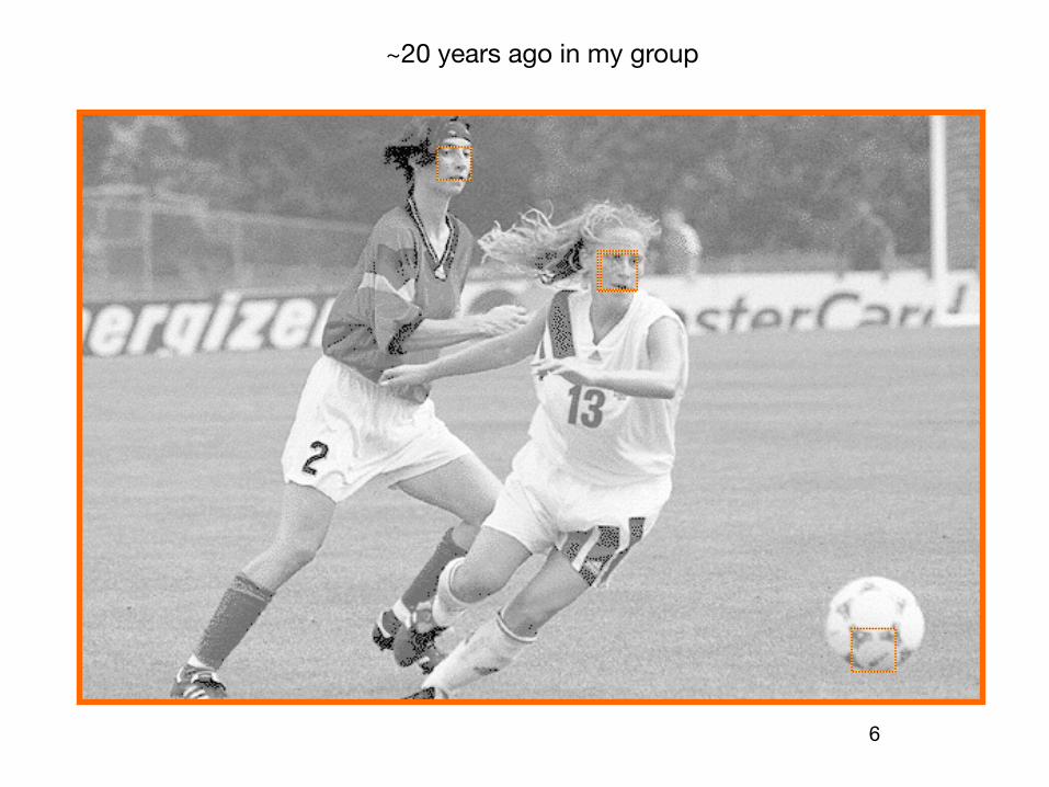
~20 years ago in my group

7
~17 years ago in my group

8

9

10

Levels of Understanding (1977--2012) !
Evolution !
Learning and development !
Computation !
Algorithms !
Wetware, hardware, circuits and components
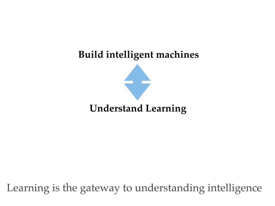
Build intelligent machines
Understand Learning
Learning is the gateway to understanding intelligence
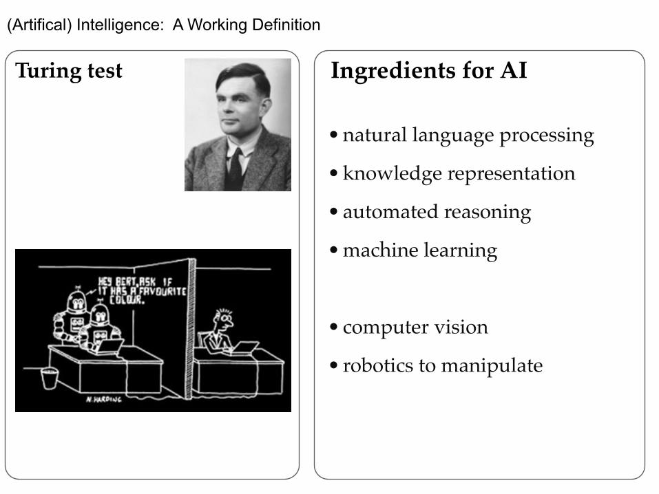
(Artifical) Intelligence: A Working Definition
Turing test Ingredients for AI
• natural language processing !
• knowledge representation!
• automated reasoning !
• machine learning !
!• computer vision!
• robotics to manipulate
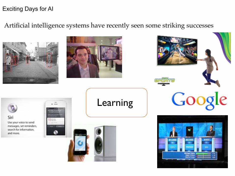
Exciting Days for AI
Artificial intelligence systems have recently seen some striking successes
Learning

ML and AI
Machine Learning
systems are trained on examples
rather than being programmed

DataUnsupervised
Feature Learning
Classic Supervised Learning
Learning Structure
Dynamic Learning
Machine Learning Problems and Approaches!
…..
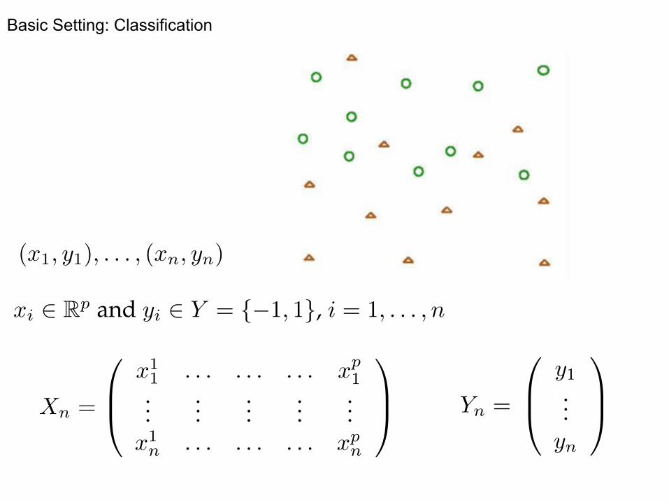
Basic Setting: Classification
Xn =
0
B@x
11 . . . . . . . . . x
p1
......
......
...x
1n . . . . . . . . . x
pn
1
CA Yn =
0
1
CA
(x1, y1), . . . , (xn, yn)
xi 2 Rp and yi 2 Y = {�1, 1}, i = 1, . . . , n

Genomics
...
;
...
n patients p gene expression measurements
Xn =
0
B@x
11 . . . . . . . . . x
p1
......
......
...x
1n . . . . . . . . . x
pn
1
CA Yn =
0
1
CA;

Text Classification: Bag of Words
Xn =
0
B@x
11 . . . . . . . . . x
p1
......
......
...x
1n . . . . . . . . . x
pn
1
CA

Image Classification
......
......
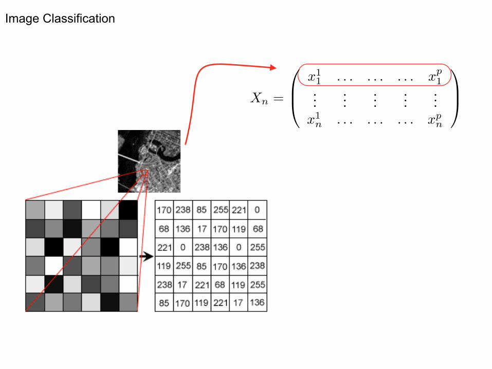
Image Classification
Xn =
0
B@x
11 . . . . . . . . . x
p1
......
......
...x
1n . . . . . . . . . x
pn
1
CA

Video Classification: Action Recognition
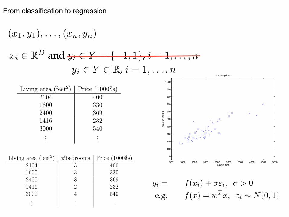
From classification to regression
(x1, y1), . . . , (xn, yn)
xi 2 RD and yi 2 Y = {�1, 1}, i = 1, . . . , n
yi 2 Y 2 R, i = 1, . . . , n
CS229 Lecture notes
Andrew Ng
Supervised learning
Let’s start by talking about a few examples of supervised learning problems.Suppose we have a dataset giving the living areas and prices of 47 housesfrom Portland, Oregon:
Living area (feet2) Price (1000$s)2104 4001600 3302400 3691416 2323000 540...
...
We can plot this data:
500 1000 1500 2000 2500 3000 3500 4000 4500 5000
0
100
200
300
400
500
600
700
800
900
1000
housing prices
square feet
pric
e (in
$10
00)
Given data like this, how can we learn to predict the prices of other housesin Portland, as a function of the size of their living areas?
1
CS229 Lecture notes
Andrew Ng
Supervised learning
Let’s start by talking about a few examples of supervised learning problems.Suppose we have a dataset giving the living areas and prices of 47 housesfrom Portland, Oregon:
Living area (feet2) Price (1000$s)2104 4001600 3302400 3691416 2323000 540...
...
We can plot this data:
500 1000 1500 2000 2500 3000 3500 4000 4500 5000
0
100
200
300
400
500
600
700
800
900
1000
housing prices
square feetpr
ice
(in $
1000
)
Given data like this, how can we learn to predict the prices of other housesin Portland, as a function of the size of their living areas?
1
3
Part I
Linear Regression
To make our housing example more interesting, let’s consider a slightly richerdataset in which we also know the number of bedrooms in each house:
Living area (feet2) #bedrooms Price (1000$s)2104 3 4001600 3 3302400 3 3691416 2 2323000 4 540...
......
Here, the x’s are two-dimensional vectors in R2. For instance, x(i)1 is the
living area of the i-th house in the training set, and x(i)2 is its number of
bedrooms. (In general, when designing a learning problem, it will be up toyou to decide what features to choose, so if you are out in Portland gatheringhousing data, you might also decide to include other features such as whethereach house has a fireplace, the number of bathrooms, and so on. We’ll saymore about feature selection later, but for now let’s take the features asgiven.)
To perform supervised learning, we must decide how we’re going to rep-resent functions/hypotheses h in a computer. As an initial choice, let’s saywe decide to approximate y as a linear function of x:
hθ(x) = θ0 + θ1x1 + θ2x2
Here, the θi’s are the parameters (also called weights) parameterizing thespace of linear functions mapping from X to Y . When there is no risk ofconfusion, we will drop the θ subscript in hθ(x), and write it more simply ash(x). To simplify our notation, we also introduce the convention of lettingx0 = 1 (this is the intercept term), so that
h(x) =n!
i=0
θixi = θTx,
where on the right-hand side above we are viewing θ and x both as vectors,and here n is the number of input variables (not counting x0).
yi = f(xi) + �"i, � > 0
e.g. f(x) = w
Tx, "i ⇠ N(0, 1)
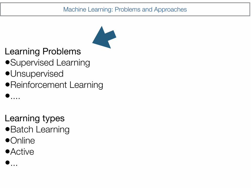
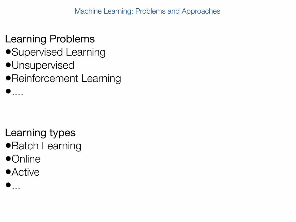
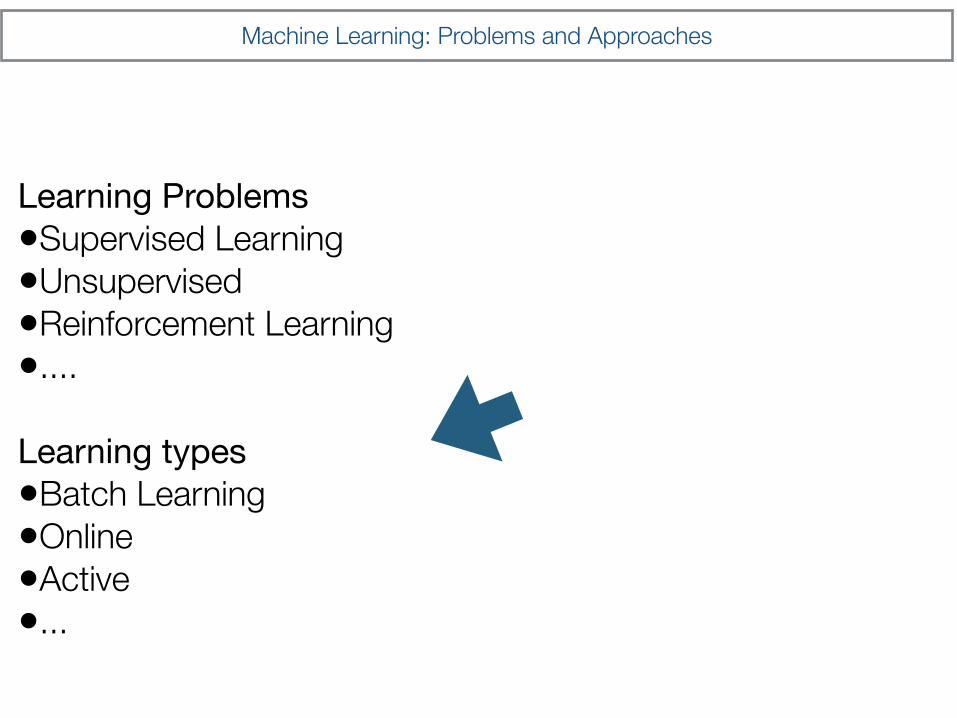
Machine Learning: Problems and Approaches
!Learning Problems•Supervised Learning •Unsupervised •Reinforcement Learning •.... !
Learning types•Batch Learning •Online •Active •... !
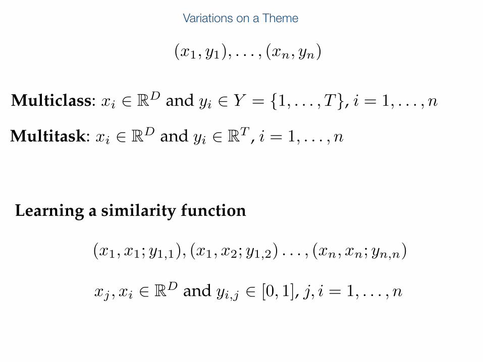
Variations on a Theme
(x1, y1), . . . , (xn, yn)
Multiclass: xi 2 RD and yi 2 Y = {1, . . . , T}, i = 1, . . . , n
Multitask: xi 2 RD and yi 2 RT , i = 1, . . . , n
(x1, x1; y1,1), (x1, x2; y1,2) . . . , (xn, xn; yn,n)
xj , xi 2 RD and yi,j 2 [0, 1], j, i = 1, . . . , n
Learning a similarity function

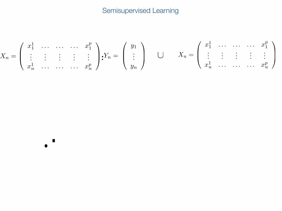
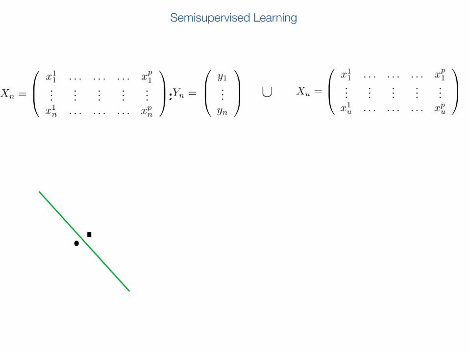
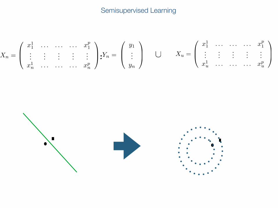
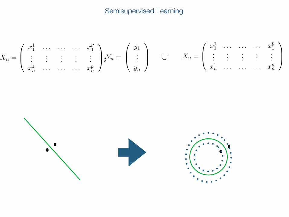
Semisupervised Learning
Xu =
0
B@x
11 . . . . . . . . . x
p1
......
......
...x
1u . . . . . . . . . x
pu
1
CA[Xn =
0
B@x
11 . . . . . . . . . x
p1
......
......
...x
1n . . . . . . . . . x
pn
1
CA Yn =
0
1
CA;
Semisupervised Learning
Xu =
0
B@x
11 . . . . . . . . . x
p1
......
......
...x
1u . . . . . . . . . x
pu
1
CA[Xn =
0
B@x
11 . . . . . . . . . x
p1
......
......
...x
1n . . . . . . . . . x
pn
1
CA Yn =
0
1
CA;
Semisupervised Learning
Xu =
0
B@x
11 . . . . . . . . . x
p1
......
......
...x
1u . . . . . . . . . x
pu
1
CA[Xn =
0
B@x
11 . . . . . . . . . x
p1
......
......
...x
1n . . . . . . . . . x
pn
1
CA Yn =
0
1
CA;
Semisupervised Learning
Xu =
0
B@x
11 . . . . . . . . . x
p1
......
......
...x
1u . . . . . . . . . x
pu
1
CA[Xn =
0
B@x
11 . . . . . . . . . x
p1
......
......
...x
1n . . . . . . . . . x
pn
1
CA Yn =
0
1
CA;
Semisupervised Learning
Xu =
0
B@x
11 . . . . . . . . . x
p1
......
......
...x
1u . . . . . . . . . x
pu
1
CA[Xn =
0
B@x
11 . . . . . . . . . x
p1
......
......
...x
1n . . . . . . . . . x
pn
1
CA Yn =
0
1
CA;
Semisupervised Learning
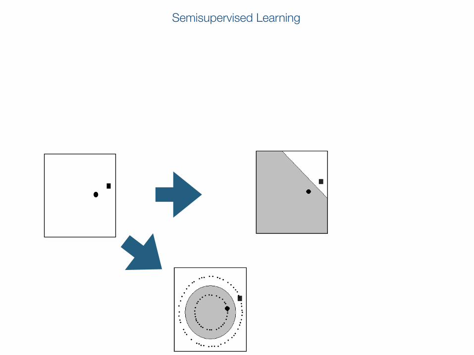
The importance of unlabeled data
L. Rosasco Manifold Regularization
The importance of unlabeled data
L. Rosasco Manifold Regularization
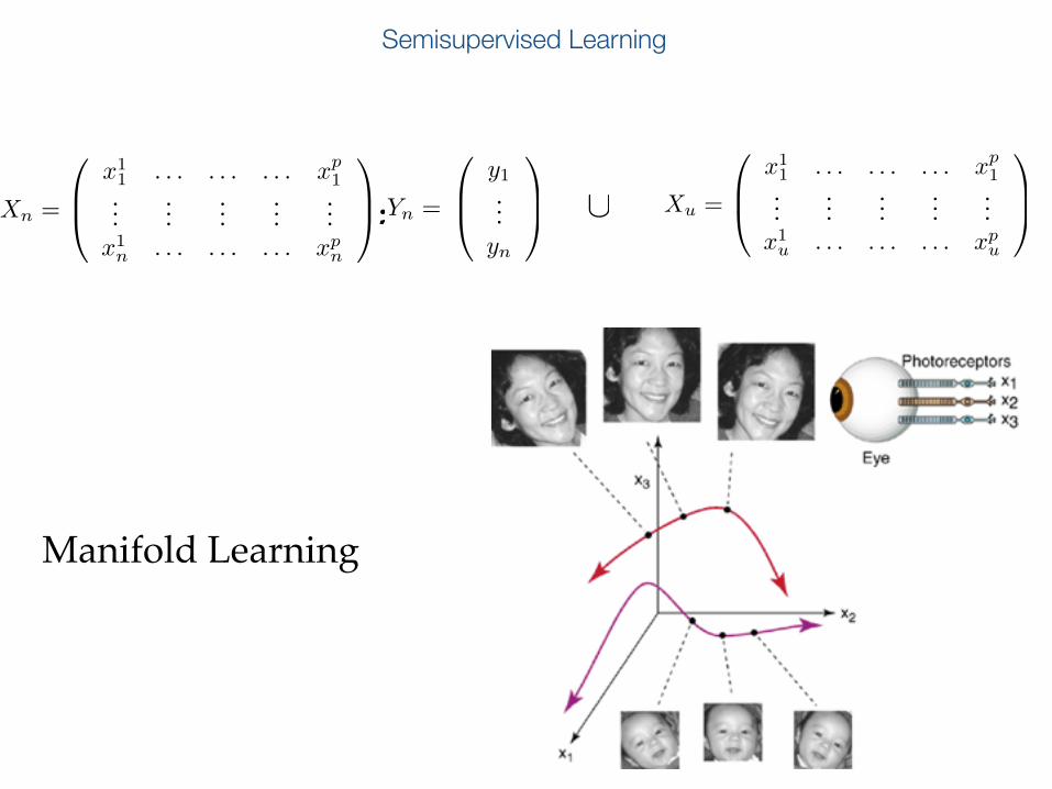
Semisupervised Learning
Xu =
0
B@x
11 . . . . . . . . . x
p1
......
......
...x
1u . . . . . . . . . x
pu
1
CA[Xn =
0
B@x
11 . . . . . . . . . x
p1
......
......
...x
1n . . . . . . . . . x
pn
1
CA Yn =
0
1
CA;
Manifold Learning

Unsupervised Learning
Clustering, k-means!Vector Quantization!Dimensionality reduction!....
Goal: Extract patterns...
Xn =
0
B@x
11 . . . . . . . . . x
p1
......
......
...x
1n . . . . . . . . . x
pn
1
CA Yn =
0
1
CA
x1, . . . , xnGiven
Machine Learning: Problems and Approaches
!Learning Problems•Supervised Learning •Unsupervised •Reinforcement Learning •.... !!Learning types•Batch Learning •Online •Active •... !
Machine Learning: Problems and Approaches
!Learning Problems•Supervised Learning •Unsupervised •Reinforcement Learning •.... !
Learning types•Batch Learning •Online •Active •... !

Online/Incremental Learning
(x1, y1)
(x2, y2)
(xn, yn)
. . .
f1
f0
f2. . .
fn (x1, y1)
f1
(x1, y1), . . . , (xn, yn)
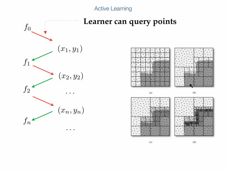
Active Learning
(x1, y1)
(x2, y2)
(xn, yn)
. . .
f1
f0
f2 . . .
fn
196 FOUNDATIONS AND APPLICATIONS OF SENSOR MANAGEMENT
(a) (b)
(c) (d)
Figure 8.7. The two step procedure for d = 2: (a) Initial unpruned RDP and n/2 samples.(b) Preview step RDP. Note that the cell with the arrow was pruned, but it contains a part of theboundary. (c) Additional sampling for the refinement step. (d) Refinement step.
The final estimator is constructed assembling the estimate “away” from theboundary obtained in the preview step with the estimate in the vicinity of theboundary obtained in the refinement step.
To formally show that this algorithm attains the faster rates we desire wehave to consider a further technical assumption, namely that the boundary setis “cusp-free”2. This condition is rather technical, but it is not very restrictive,and encompasses many interesting situations, including of course, boundaryfragments. This condition seems to be necessary for the algorithm to performwell, and it is not simply an artifact of the proof. For a more detailed explana-tion see [52]. Under this condition we have the following theorem.
2A cusp-free boundary cannot have the behavior you observe in the graph of |x|1/2 at the origin. Less“aggressive” kinks are allowed, such as in the graph of |x|.
Learner can query points

Summary
We look for systems that are trained, rather than programmed, to perform a task !Learning from examples is a unifying paradigm in learning: !
``Learning is the acquisition of knowledge or skills through study, experience, or being taught’’


![APPENDIX B Math Handbook Math Handbook - …glencoe.mheducation.com/.../179000/math_handbook.pdfThus, [H ] antilog( 9.54) 10 9.54 100.46 ( 10) 100.46 10 10 2.9 10 10M Check the instruction](https://static.fdocuments.us/doc/165x107/5ae560237f8b9aee078b7387/appendix-b-math-handbook-math-handbook-h-antilog-954-10-954-10046.jpg)