
9/20/2004 10:43 AM 1 Statistical Methods for Recognition Statistical
35
9/20/2004 10:43 AM 1 Statistical Methods for Recognition Statistical Methods for the Recognition and Understanding of Speech 1 Lawrence R. Rabiner* & B.H. Juang # * Rutgers University and the University of California, Santa Barbara # Georgia Institute of Technology, Atlanta Abstract Statistical methods for speech processing refer to a general methodology in which knowledge about both a speech signal and the language that it expresses, along with practical uses of that knowledge for specific tasks or services, is developed from actual realizations of speech data through a well-defined mathematical and statistical formalism. For more than 20 years, this basic methodology has produced many advances and new results, particularly for recognizing and understanding speech and natural language by machine. In this article, we focus on several important statistical methods, e.g., one based primarily on the hidden Markov model (HMM) formulation that has gained widespread acceptance as the dominant technique and one related to use of statistics for characterizing word co-occurrences. In order to recognize and understand speech, the speech signal is first processed by an acoustic processor, which converts the waveform to a set of spectral feature vectors which characterize the time-varying properties of the speech sounds, and then by a linguistic decoder, which decodes the feature vectors into a word sequence which is valid according to the word lexicon and task grammar associated with the speech recognition or understanding task. The hidden Markov model approach is mainly used for acoustic modeling, that is assigning probabilities to acoustic realizations of a sequence of sounds or words, and a statistical language model is used to assign probabilities to sequences of words in the language. A Bayesian approach is used to find the word sequence with the maximum a posteriori probability over all possible sentences in the task language. This search problem is often astronomically large for large vocabulary speech understanding problems, and thus the speech-to-text decoding process often requires inordinate amounts of computing power to solve by heuristic methods. Fortunately, using results from the field of Finite State Automata Theory, we can reduce the computational burden of the search by orders of magnitude, thereby enabling exact solutions in computationally feasible times for large speech recognition problems. 1 This article is based on a series of lectures on Challenges in Speech Recognition by one of the authors (LRR) and his many colleagues at AT&T Labs Research, most especially Dr. Mazin Rahim who contributed to the presentation and figures used throughout this article. We thank Dr. Rahim for his help and support.
Transcript of 9/20/2004 10:43 AM 1 Statistical Methods for Recognition Statistical

9/20/2004 10:43 AM 1 Statistical Methods for Recognition
Statistical Methods for the Recognition and Understanding of Speech1
Lawrence R. Rabiner* & B.H. Juang#
* Rutgers University and the University of California, Santa Barbara # Georgia Institute of Technology, Atlanta
Abstract Statistical methods for speech processing refer to a general methodology in which knowledge
about both a speech signal and the language that it expresses, along with practical uses of that
knowledge for specific tasks or services, is developed from actual realizations of speech data
through a well-defined mathematical and statistical formalism. For more than 20 years, this basic
methodology has produced many advances and new results, particularly for recognizing and
understanding speech and natural language by machine. In this article, we focus on several
important statistical methods, e.g., one based primarily on the hidden Markov model (HMM)
formulation that has gained widespread acceptance as the dominant technique and one related to
use of statistics for characterizing word co-occurrences. In order to recognize and understand
speech, the speech signal is first processed by an acoustic processor, which converts the
waveform to a set of spectral feature vectors which characterize the time-varying properties of the
speech sounds, and then by a linguistic decoder, which decodes the feature vectors into a word
sequence which is valid according to the word lexicon and task grammar associated with the
speech recognition or understanding task. The hidden Markov model approach is mainly used for
acoustic modeling, that is assigning probabilities to acoustic realizations of a sequence of sounds
or words, and a statistical language model is used to assign probabilities to sequences of words in
the language. A Bayesian approach is used to find the word sequence with the maximum a
posteriori probability over all possible sentences in the task language. This search problem is
often astronomically large for large vocabulary speech understanding problems, and thus the
speech-to-text decoding process often requires inordinate amounts of computing power to solve
by heuristic methods. Fortunately, using results from the field of Finite State Automata Theory,
we can reduce the computational burden of the search by orders of magnitude, thereby enabling
exact solutions in computationally feasible times for large speech recognition problems.
1 This article is based on a series of lectures on Challenges in Speech Recognition by one of the authors (LRR) and his many colleagues at AT&T Labs Research, most especially Dr. Mazin Rahim who contributed to the presentation and figures used throughout this article. We thank Dr. Rahim for his help and support.

9/20/2004 10:43 AM 2 Statistical Methods for Recognition
1. Introduction
The goal of getting a machine to understand fluently spoken speech and respond in a natural
voice has been driving speech research for more than 50 years. Although the personification of an
intelligent machine such as Hal in the movie 2001, A Space Odyssey, or R2D2 in the Star Wars
series, has been around for more than 35 years, we are still not yet at the point where machines
reliably understand fluent speech, spoken by anyone, and in any acoustic environment. In spite of
the remaining technical problems that need to be solved, the fields of automatic speech
recognition and understanding have made tremendous advances and the technology is now
readily available and used on a day-to-day basis in a number of applications and services—
especially those conducted over the public-switched telephone network (PSTN) [1]. This article
aims at reviewing the technology that has made these applications possible.
Speech recognition and language understanding are two major research thrusts that have
traditionally been approached as problems in linguistics and acoustic-phonetics, where a range of
acoustic-phonetic knowledge has been brought to bear on the problem with remarkably little
success. In this article, however, we focus on statistical methods for speech and language
processing, where the knowledge about a speech signal and the language that it expresses,
together with practical uses of the knowledge, is developed from actual realizations of speech
data through a well-defined mathematical and statistical formalism. We review how the statistical
methods are used for speech recognition and language understanding, show current performance
on a number of task specific applications and services, and discuss the challenges that remain to
be solved before the technology becomes ubiquitous.
2. The Speech Advantage
There are fundamentally three major reasons why so much research and effort has gone into
the problem of trying to teach machines to recognize and understand fluent speech, and these are
the following:
• Cost reduction – Among the earliest goals for speech recognition systems was to replace
humans, who were performing some simple tasks, with automated machines, thereby
reducing labor expenses while still providing customers with a natural and convenient
way to access information and services. One simple example of a cost reduction system
was the Voice Recognition Call Processing (VRCP) system introduced by AT&T in 1992
[2] which essentially automated so-called “Operator Assisted” calls, such as Person-to-
Person calls, Reverse billing calls, Third Party Billing calls, Collect Calls (by far the most

9/20/2004 10:43 AM 3 Statistical Methods for Recognition
common class of such calls), and Operator-Assisted Calls. The resulting automation
eliminated about 6600 jobs, while providing a quality-of-service that matched or
exceeded that provided by the live attendants, saving AT&T on the order of $300M per
year.
• New revenue opportunities – speech recognition and understanding systems enabled
service providers to have a 24x7 high quality customer care automation capability,
without the need for access to information by keyboard or touch tone button pushes. An
example of such a service was the How May I Help You (HMIHY) service introduced by
AT&T late in 1999 [3] which automated the customer care for AT&T Consumer
Services. This system will be discussed further in the section on speech understanding. A
second example of such a service was the NTT Anser service for voice banking in Japan
[4], which enabled Japanese banking customers to access bank account records from an
ordinary telephone without having to go to the bank. (Of course, today we utilize the
Internet for such information, but in 1988, when this system was introduced, the only
way to access such records was a physical trip to the bank and a wait in lines to speak to a
banking clerk.)
• Customer retention – speech recognition provides the potential for personalized services
based on customer preferences, and thereby to improve the customer experience. A trivial
example of such a service is the voice-controlled automotive environment which
recognizes the identity of the driver from voice commands and adjusts the automobile’s
features (seat position, radio station, mirror positions, etc.) to suit the customer preference
(which is established in an enrollment session).
3. The Speech Dialog Circle
When we consider the problem of communicating with a machine, we must consider the
cycle of events that occurs between a spoken utterance (as part of a dialog between a person and a
machine) and the response to that utterance from the machine. Figure 1 shows such a sequence of
events, which is often referred to as “The Speech Dialog Circle”, using an example in the
telecommunication context.

9/20/2004 10:43 AM 4 Statistical Methods for Recognition
Figure 1—The Conventional Speech Dialog Circle
The customer initially makes a request by speaking an utterance which is sent to a machine
which attempts to recognize, on a word-by-word basis, the spoken speech. The process of
recognizing the words in the speech is called Automatic Speech Recognition (ASR) and its output
is an orthographic representation of the recognized spoken input. The ASR process will be
discussed in the next section. Next the spoken words are analyzed by a Spoken Language
Understanding (SLU) module which attempts to attribute meaning to the spoken words. The
meaning that is attributed is in the context of the task being handled by the speech dialog system.
(What is described here is traditionally referred to as a limited domain understanding system or
application,) Once meaning has been determined, the Dialog Management (DM) module
examines the state of the dialog according to a prescribed operational workflow and determines
the course of action that would be most appropriate to take. The action may be as simple as a
request for further information or confirmation of an action that is taken. Thus if there were
confusion as to how best to proceed, a text query would be generated by the Spoken Language
Generation module to hopefully clarify the meaning and help determine what to do next. The
query text is then sent to the final module, the Text-to-Speech Synthesis (TTS) module, and then
Data
DM
SLG SLU
ASR TTS
Meaning “Billing credit”
Words spoken “I dialed a wrong number”
Workflow, context& actions to take
Automatic Speech
Recognition
Spoken Language
Understanding
Text-to-Speech
Synthesis
Spoken Language Generation
Reply to customer “What number did you want to
call?” in a synthetic voice
Spoken Customer Request
call?
Dialog Management
Sound pressure waveform
Workflow – determine number: “What number did you want to

9/20/2004 10:43 AM 5 Statistical Methods for Recognition
converted into intelligible and highly natural speech which is sent to the customer who decides
what to say next based on what action was taken, or based on previous dialogs with the machine.
All of the modules in the Speech Dialog Circle can be “data-driven” in both the learning and
active use phases, as indicated by the central Data block in Figure 1.
A typical task scenario, e.g., booking an airline reservation, requires navigating the Speech
Dialog Circle many times – each time being referred to as one “turn” - to complete a transaction.
(The average number of turns a machine takes to complete a prescribed task is a measure of the
effectiveness of the machine in many applications.) Hopefully, each time through the dialog
circle enables the customer to get closer to the desired action either via proper understanding of
the spoken request or via a series of clarification steps. The speech dialog circle is a powerful
concept in modern speech recognition and understanding systems, and is at the heart of most
speech understanding systems that are in use today.
4. Basic ASR Formulation
The goal of an ASR system is to accurately and efficiently convert a speech signal into a text
message transcription of the spoken words, independent of the device used to record the speech
(i.e., the transducer or microphone), the speaker, or the environment. A simple model of the
speech generation process, as used to convey a speaker’s intention is shown in Figure 2.
Figure 2 – Model of Spoken Speech
It is assumed that the speaker decides what to say and then embeds the concept in a sentence, W ,
which is a sequence of words (possibly with pauses and other acoustic events such as uh’s, um’s,
er’s, etc.) The speech production mechanisms then produce a speech waveform, ( )s n , which
embodies the words of W as well as the extraneous sounds and pauses in the spoken input. A
conventional automatic speech recognizer attempts to decode the speech, ( )s n , into the best
estimate of the sentence, W , using a two-step process, as shown in Figure 3.
Linguistic Composition
Speech Production
Speaker’s Intention
W s(n)
Context & Focus

9/20/2004 10:43 AM 6 Statistical Methods for Recognition
Figure 3 – ASR Decoder from speech to sentence
The first step in the process is to convert the speech signal, ( )s n , into a sequence of spectral
feature vectors, X , where the feature vectors are measured every 10 ms (or so) throughout the
duration of the speech signal. The second step in the process is to use a syntactic decoder to
generate every possible valid sentence (as a sequence of orthographic representations) in the task
language, and to evaluate the score (i.e., the a posteriori probability of the word string given the
realized acoustic signal as measured by the feature vector) for each such string, choosing as the
recognized string, W , the one with the highest score. This is the so-called maximum a posteriori
probability (MAP) decision principle, originally suggested by Bayes. Additional linguistic
processing can be done to try to determine side information about the speaker, such as the
speaker’s intention, as indicated in Figure 3.
Mathematically, we seek to find the string W that maximizes the a posteriori probability of
that string, when given the measured feature vector X, i.e.,
)|(maxargˆ XWPWW
=
Using Bayes Law, we can rewrite this expression as:
)()()|(maxargˆ
XPWPWXPW
W=
Thus, calculation of the a posteriori probability is decomposed into two main components, one
that defines the a priori probability of a word sequence W, P(W), and the other the likelihood of
the word string W in producing the measured feature vector, P(X|W). (We disregard the
denominator term, ( )P x , since it is independent of the unknown W . The former is referred to as
W
Syntactic constraints
Context & Focus Conventional Automatic Speech Recognizer
Syntactical Decoding
s(n) Acoustic Processing
Speaker’s intention X Linguistic
Parsing

9/20/2004 10:43 AM 7 Statistical Methods for Recognition
the Acoustic Model, ( | )AP X W , and the latter the Language Model, ( )LP W [5-6]. We note that
these quantities are not given directly, but instead are usually estimated or inferred from a set of
training data that have been labeled by a knowledge source, i.e., a human expert. The decoding
equation is then rewritten as:
ˆ arg max ( | ) ( )A LWW P X W P W=
We explicitly write the sequence of feature vectors (the acoustic observations) as:
NX xxx ,,, 21 L= where the speech signal duration is N frames (or N times 10 msec. when the frame shift is 10
msec). Similarly we explicitly write the optimally decoded word sequence as:
MwwwW L21ˆ =
where there are M words in the decoded string. The above decoding equation defines the
fundamental statistical approach to the problem of automatic speech recognition.
It can be seen that there are three steps to the basic ASR formulation, namely:
Step 1 – acoustic modeling for assigning probabilities to acoustic (spectral) realizations of a
sequence of words. For this step we use a statistical model (called the hidden
Markov model or HMM) of the acoustic signals of either individual words or sub-
word units (e.g., phonemes) to compute the quantity ( | )AP X W . We train the
acoustic models from a training set of speech utterances, which have been
appropriately labeled to establish the statistical relationship between X and W.
Step 2 – language modeling for assigning probabilities, ( )LP W , to sequences of words that
form valid sentences in the language and are consistent with the recognition task
being performed. We train such language models from generic text sequences, or
from transcriptions of task specific dialogues.
Step 3 – hypothesis search whereby we find the word sequence with the maximum a
posterior probability by searching through all possible word sequences in the
language.
a) Notes on Step 1 – the Acoustic Model [7-8]
9/20/2004 10:43 AM 8 Statistical Methods for Recognition
We train a set of acoustic models for the words or sounds of the language by learning the
statistics of the acoustic features, X, for each word or sound, from a speech training set,
where we compute the variability of the acoustic features during the production of the
words or sounds, as represented by the models. For large vocabulary tasks, it is
impractical to create a separate acoustic model for every possible word in the language
since it requires far too much training data to measure the variability in every possible
context. Instead we train a set of about 50 acoustic-phonetic sub-word models for the ~50
phonemes in the English language, and construct a model for a word by concatenating
(stringing together sequentially) the models for the constituent sub-word sounds in the
word, as defined in a word lexicon or dictionary, where multiple pronunciations are
allowed). Similarly we build sentences (sequences of words) by concatenating word
models. Since the actual pronunciation of a phoneme may be influenced by neighboring
phonemes (those occurring before and after the phoneme), the set of so-called “context-
dependent” phoneme models are often used as the speech models, as long as sufficient
data are collected for proper training of these models.
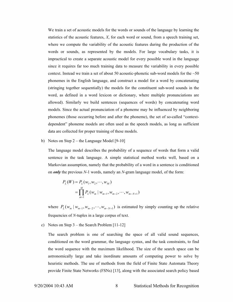
b) Notes on Step 2 – the Language Model [9-10]
The language model describes the probability of a sequence of words that form a valid
sentence in the task language. A simple statistical method works well, based on a
Markovian assumption, namely that the probability of a word in a sentence is conditioned
on only the previous N-1 words, namely an N-gram language model, of the form:
∏=
+−−−=
=M
mNmmmmL
MLL
wwwwP
wwwPWP
1121
21
),,,|(
),,,()(
L
L
where ),,,|( 121 +−−− NmmmmL wwwwP L is estimated by simply counting up the relative
frequencies of N-tuples in a large corpus of text.
c) Notes on Step 3 – the Search Problem [11-12]
The search problem is one of searching the space of all valid sound sequences,
conditioned on the word grammar, the language syntax, and the task constraints, to find
the word sequence with the maximum likelihood. The size of the search space can be
astronomically large and take inordinate amounts of computing power to solve by
heuristic methods. The use of methods from the field of Finite State Automata Theory
provide Finite State Networks (FSNs) [13], along with the associated search policy based

9/20/2004 10:43 AM 9 Statistical Methods for Recognition
on dynamic programming, that reduce the computational burden by orders of magnitude,
thereby enabling exact solutions in computationally feasible times, for large speech
recognition problems.
5. Development of a Speech Recognition System for a Task or an Application
Before going into more details on the various aspects of the process of Automatic Speech
Recognition by machine, we review the 3 steps that must occur in order to define, train, and build
an ASR system [14-15]. These steps are the following:
Step 1 Choose the recognition task – specify the word vocabulary for the task, the set of units
that will be modeled by the acoustic models (e.g., whole words, phonemes, etc.), the
word pronunciation lexicon (or dictionary) that describes the variations in word
pronunciation, the task syntax (grammar), and the task semantics. By way of example,
for a simple speech recognition system capable of recognizing a spoken credit card
number using isolated digits (i.e., single digits spoken one at a time), the sounds to be
recognized are either whole words or the set of sub-word units that appear in the digits
/zero/ to /nine/ plus the word /oh/. The word vocabulary is the set of 11 digits. The task
syntax allows any single digit to be spoken, and the task semantics specify that a
sequence of isolated digits must form a valid credit card code for identifying the user.
Step 2 Train the models – create a method for building acoustic word models (or sub-word
models) from a labeled speech training data set of multiple occurrences of each of the
vocabulary words by one or more speakers. We also must use a text training data set to
create a word lexicon (dictionary) describing the ways that each word can be
pronounced (assuming we are using sub-word units to characterize individual words), a
word grammar (or language model) that describes how words are concatenated to form
valid sentences (i.e., credit card numbers), and finally a task grammar that describes
which valid word strings are meaningful in the task application (e.g., valid credit card
numbers).
Step 3 Evaluate recognizer performance – we need to determine the word error rate and the
task error rate for the recognizer on the desired task. For an isolated digit recognition
task, the word error rate is just the isolated digit error rate, whereas the task error rate
would be the number of credit card errors that lead to mis-identification of the user.
Evaluation of the recognizer performance often includes an analysis of the types of
recognition errors made by the system. This analysis can lead to revision of the task in

9/20/2004 10:43 AM 10 Statistical Methods for Recognition
a number of ways, ranging from changing the vocabulary words or the grammar (i.e., to
eliminate highly confusable words) to the use of word-spotting, as opposed to word
transcription. As an example, in limited vocabulary applications, if the recognizer
encounters frequent confusions between words like “freight” and “flight,” it may be
advisable to change “freight” to “cargo” to maximize its distinction from “flight.”
Revision of the task grammar often becomes necessary if the recognizer experiences
substantial amounts of what is called “out of grammar” (OOG) utterances, namely the
use of words and phrases that are not directly included in the task vocabulary [16].
6. The Speech Recognition Process
In this section, we provide some technical aspects of a typical speech recognition system.
Figure 4 shows a block diagram of a speech recognizer that follows the Bayesian framework
discussed above.
Figure 4 – Framework of ASR System
The recognizer consists of three processing steps, namely Feature Analysis, Pattern Matching
and Confidence Scoring, along with three trained databases, the set of Acoustic Models, the Word
Lexicon and the Language Model. In this section we briefly describe each of the processing steps
and each of the trained model databases.
a. Feature Analysis
W
Feature Analysis (Spectral Analysis)
Input Speech
s(n), W
Pattern Matching
(Decoding, Search)
AcousticModel (HMM)
Confidence Scoring
(Utterance Verification)
“Hello World”
(0.9) (0.8)
Word Lexicon
LanguageModel
(N-gram)
9/20/2004 10:43 AM 11 Statistical Methods for Recognition
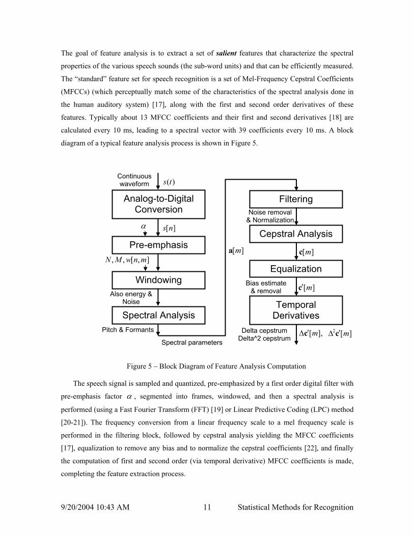
The goal of feature analysis is to extract a set of salient features that characterize the spectral
properties of the various speech sounds (the sub-word units) and that can be efficiently measured.
The “standard” feature set for speech recognition is a set of Mel-Frequency Cepstral Coefficients
(MFCCs) (which perceptually match some of the characteristics of the spectral analysis done in
the human auditory system) [17], along with the first and second order derivatives of these
features. Typically about 13 MFCC coefficients and their first and second derivatives [18] are
calculated every 10 ms, leading to a spectral vector with 39 coefficients every 10 ms. A block
diagram of a typical feature analysis process is shown in Figure 5.
Figure 5 – Block Diagram of Feature Analysis Computation
The speech signal is sampled and quantized, pre-emphasized by a first order digital filter with
pre-emphasis factor α , segmented into frames, windowed, and then a spectral analysis is
performed (using a Fast Fourier Transform (FFT) [19] or Linear Predictive Coding (LPC) method
[20-21]). The frequency conversion from a linear frequency scale to a mel frequency scale is
performed in the filtering block, followed by cepstral analysis yielding the MFCC coefficients
[17], equalization to remove any bias and to normalize the cepstral coefficients [22], and finally
the computation of first and second order (via temporal derivative) MFCC coefficients is made,
completing the feature extraction process.
Continuous waveform
Noise removal & Normalization
Bias estimate & removal
Analog-to-Digital Conversion
Pre-emphasis
Windowing
Spectral Analysis
Filtering
Temporal Derivatives
Equalization
Cepstral Analysis
],[,, mnwMN][ma
Also energy & Noise
Pitch & Formants
)(ts
α ][ns
][mc
],[mc′∆ ][2 mc′∆
][mc′
Delta cepstrum Delta^2 cepstrum Spectral parameters

9/20/2004 10:43 AM 12 Statistical Methods for Recognition
b. Acoustic Models
The goal of acoustic modeling is to characterize the statistical variability of the feature set
determined above for each of the basic sounds (or words) of the language. Acoustic modeling
uses probability measures to characterize sound realization using statistical models. A statistical
method, known as the hidden Markov model (HMM) [23-26], is used to model the spectral
variability of each of the basic sounds of the language using a mixture density Gaussian
distribution [27-28] which is optimally aligned with a speech training set and iteratively updated
and improved (the means, variances, and mixture gains are iteratively updated) until an optimal
alignment and match is achieved.
Figure 6 shows a simple 3-state HMM for modeling the subword unit /s/ as spoken at the
beginning of the word /six/. Each HMM state is characterized by a probability density function
(usually a mixture Gaussian density) that characterizes the statistical behavior of the feature
vectors at the beginning (state s1), middle (state s2) and end (state s3) of the sound /s/. In order to
train the HMM for each subword unit, we use a labeled training set of words and sentences and
utilize an efficient training procedure known as the Baum-Welch algorithm [25, 29-30] to align
each of the various subword units with the spoken inputs, and then estimate the appropriate
means, covariances, and mixture gains for the distributions in each subword unit state. The
algorithm is a hill-climbing algorithm and is iterated until a stable alignment of subword unit
models and speech is obtained, enabling the creation of stable models for each subword unit.
Figure 7 shows how a simple two sound word, “is”, which consists of the sounds /IH/ and /Z/,
is created by concatenating the models [31] for the /IH/ sound with the model for the /Z/ sound,
thereby creating a 6-state model for the word “is”.
S1
S2
S3
3-state phone model for /s/ Figure 6 – 3-state HMM for the sound /s/

9/20/2004 10:43 AM 13 Statistical Methods for Recognition
Figure 8 shows how an HMM can be used to characterize a whole word model [32]. In
this case the word is modeled as a sequence of 5 HMM states, where each state is characterized
by a mixture density, denoted as )( tjb x where the model state is the index j, the feature vector at
time t is denoted as tx , and the mixture density is of the form:
[ ]
Njdb
Njc
jkU
jkµ
cjkcK
Dxxx
Ucb
ttj
K
k jk
jk
jk
jkth
jk
tDttt
jkjkt
K
kjktj
≤≤=
≤≤=
=
==
≥=
===
=
∫∑
∑
∞
∞−
=
=
1,1)(
1,1
0,
39),,,,(
,,)(
1
21
1
xx
x
xx
state , mixture formatrix covariance state , mixture for vector mean
functiondensity Gaussian state in component mixture of weight
functiondensity the in components mixture of number
N
N
L
µ
1 2 3 4 5
11a 22a 33a 44a 55a
12a 23a 34a 45a
13a 24a 35a
)(1 tb x )(2 tb x )(3 tb x )(4 tb x
Figure 8 HMM for whole word model with 5 states
)(5 tb x
‘ih’
ih1
ih2
ih3
‘z’
z1
z2
z3
Figure 7 Concatenated model for the word “is.”

9/20/2004 10:43 AM 14 Statistical Methods for Recognition
Included in Figure 8 are an explicit set of state transitions, ija , which specify the probability
of making a transition from state i to state j at each frame, thereby defining the time sequence of
the feature vectors over the duration of the word. Usually the self-transitions, iia , are large (close
to 1.0), and the skip-state transitions, 13 24 35, ,a a a , are small (close to 0).
Once the set of state transitions and state probability densities are specified, we say that a
model λ (which is also used to denote the set of parameters that define the probability measure)
has been created for the word or subword unit. In order to optimally train the various models (for
each word unit [32] or subword unit [31]), we need to have algorithms that perform the following
three steps or tasks [26] using the acoustic observation sequence, X, and the model λ :
a. Likelihood Evaluation: compute )|( λXP
b. Decoding: choose the optimal state sequence for a given speech utterance
c. Re-estimation: adjust the parameters of λ to maximize )|( λXP
Figure 9 – The Baum-Welch Training Procedure
Each of these three steps is essential to defining the optimal HMM models for speech
recognition based on the available training data and each task if approached in a brute force
manner would be computationally costly. Fortunately efficient algorithms have been developed
to enable efficient and accurate solutions to each of the three steps that must be performed to train
and utilize HMM models in a speech recognition system. These are generally referred to as the
forward-backward algorithm or the Baum-Welch reestimation method [23]. Details of the Baum-
Compute Forward & Backward
Probabilities
Optimize Parameters
Input SpeechDatabase
Old (Initial) HMM Model jkjkjkij Uµca ,,,
Updated HMM Model
9/20/2004 10:43 AM 15 Statistical Methods for Recognition
Welch procedure are beyond the scope of this article. The heart of the training procedure for re-
estimating model parameters using the Baum-Welch procedure is shown in Figure 9.
c. Word Lexicon
The purpose of the word lexicon or dictionary is to define the range of pronunciation of
words in the task vocabulary [33-34]. The reason that such a word lexicon is necessary is because
the same orthography can be pronounced differently by people with different accents, or because
the word has multiple meanings that change the pronunciation by the context of its use. For
example the word “data” can be pronounced as: /d/ /ae/ /t/ /ax/ or as /d/ /ey/ /t/ /ax/, and we would
need both pronunciations in the dictionary to properly train the recognizer models and to properly
recognize the word when spoken by different individuals. Another example of variability in
pronunciation from orthography is the word “record” which can be either a disk that goes on a
player, or the process of creating sound. The different meanings have significantly different
pronunciations.
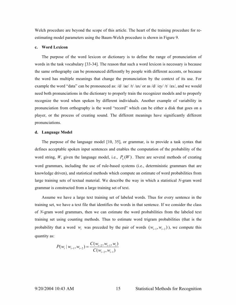
d. Language Model
The purpose of the language model [10, 35], or grammar, is to provide a task syntax that
defines acceptable spoken input sentences and enables the computation of the probability of the
word string, W, given the language model, i.e., ( )LP W . There are several methods of creating
word grammars, including the use of rule-based systems (i.e., deterministic grammars that are
knowledge driven), and statistical methods which compute an estimate of word probabilities from
large training sets of textual material. We describe the way in which a statistical N-gram word
grammar is constructed from a large training set of text.
Assume we have a large text training set of labeled words. Thus for every sentence in the
training set, we have a text file that identifies the words in that sentence. If we consider the class
of N-gram word grammars, then we can estimate the word probabilities from the labeled text
training set using counting methods. Thus to estimate word trigram probabilities (that is the
probability that a word iw was preceded by the pair of words 1 2( , )i iw w− − ), we compute this
quantity as:
2 11 2
2 1
( , , )( | , )( , )
i i ii i i
i i
C w w wP w w wC w w
− −− −
− −
=

9/20/2004 10:43 AM 16 Statistical Methods for Recognition
where 2 1( , , )i i iC w w w− − is the frequency count of the word triplet (i.e., trigram) consisting of
2 1( , , )i i iw w w− − occurred in the training set, and 2 1( , )i iC w w− − is the frequency count of the word
duplet (i.e., bigram) 2 1( , )i iw w− − occurred in the training set.
Although the method of training N-gram word grammars, as described above, generally
works quite well, it suffers from the problem that the counts of N-grams are often highly in error
due to problems of data sparseness in the training set. Hence for a text training set of millions of
words, and a word vocabulary of several thousand words, more than 50% of word trigrams are
likely to occur either once or not at all in the training set. This leads to gross distortions in the
computation of the probability of a word string, as required by the basic Bayesian recognition
algorithm. In the cases when a word trigram does not occur at all in the training set, it is
unacceptable to define the trigram probability as 0 (as would be required by the direct definition
above), since this leads to effectively invalidating all strings with that particular trigram from
occurring in recognition. Instead, in the case of estimating trigram word probabilities (or similarly
extended to N-grams where N is more than three), a smoothing algorithm [36] is applied by
interpolating trigram, bigram and unigram relative frequencies, i.e.,
2 1 11 2 3 2 1
2 1 1
3 2 1
( , , ) ( , ) ( )ˆ( | , )( , ) ( ) ( )
1
( ) size of text training corpus
i i i i i ii i i
i i i ii
ii
C w w w C w w C wP w w w p p pC w w C w C w
p p p
C w
− − −− −
− − −
= + +
+ + =
=
∑
∑
where the smoothing probabilities, 3 2 1, ,p p p are obtained by applying the principle of cross-
validation. Other schemes such as the Turing-Good estimator that deals with unseen classes of
observations in distribution estimation have also been proposed [37].
Worth mentioning here are two important notions that are associated with language models:
perplexity of the language model and the rate of occurrences of out-of-vocabulary words in real
data sets. We elaborate them below:
Language Perplexity
A measure of the complexity of the language model is the mathematical quantity known as
language perplexity (which is actually the geometric mean of the word branching factor, or the
average number of words that follow any given word of the language) [38]. We can compute

9/20/2004 10:43 AM 17 Statistical Methods for Recognition
language perplexity, as embodied in the language model, )(WPL , where
1 2( , ,..., )QW w w w= is a length-Q word sequence, by first defining the entropy [39] as:
21( ) log ( )H W P WQ
= − .
Using a trigram language model we can write the entropy as:
2 1 21
1( ) log ( | , )Q
i i ii
H W P w w wQ − −
=
= − ∑
where we suitably define the first couple of probabilities as the unigram and bigram
probabilities. Note that as Q approaches infinity, the above entropy approaches the
asymptotic entropy of the source defined by the measure )(WPL . The perplexity of the
language is then defined as:
( ) 1/1 2( ) 2 ( , ,..., )H W Q
QPP W P w w w −= = . as ∞→Q
Some examples of language perplexity for specific speech recognition tasks are the
following:
i. for an 11 digit vocabulary (“zero” to “nine” plus “oh”) where every digit can
occur independently of every other digit, the language perplexity (average word
branching factor) is 11;
ii. for a 2000 word Airline Travel Information System (ATIS) [40], the language
perplexity (using a trigram language model) is 20 [41];
iii. for a 5000 word Wall Street Journal Task (reading articles aloud) the language
perplexity (using a bigram language model) is 130 [42].
A plot of the bigram perplexity for a training set of 500 million words, tested on the Encarta
Encyclopedia is shown in Figure 10. It can be seen that language perplexity grows only
slowly with the vocabulary size and is only about 400 for a 60,000 word vocabulary.
Out-of-Vocabulary Rate
Another interesting aspect of language models is their coverage of the language as
exemplified by the concept of an Out-of-Vocabulary (OOV) [43] rate which measures how
often a new word appears for a specific task, given that a language model of a given
vocabulary size for the task has been created. Figure 11 shows the OOV rate for sentences

9/20/2004 10:43 AM 18 Statistical Methods for Recognition
from the Encarta Encyclopedia, again trained on 500 million words of text, as a function of
the vocabulary size. It can be seen that even for a 60,000-word vocabulary, about 4% of the
words that are encountered have not been seen previously and thus are considered OOV
words (which, by definition, cannot be recognized correctly by the recognition system).
Figure 10 – Bigram Language Perplexity for Encarta Encyclopedia
Figure 11 – Out-of-Vocabulary Rate of Encarta Encyclopedia as a Function of the
Vocabulary Size

9/20/2004 10:43 AM 19 Statistical Methods for Recognition
e. Pattern Matching
The job of the pattern matching module is to combine information (probabilities) from the
acoustic model, the language model and the word lexicon to find the “optimal” word sequence,
i.e., the word sequence that is consistent with the language model and that has the highest
probability among all possible word sequences in the language (i.e., best matches the spectral
feature vectors of the input signal). To achieve this goal, the pattern matching system is actually a
decoder [11-13] that searches through all possible word strings and assigns a probability score to
each string, using a Viterbi decoding algorithm [44] or its variants.
The challenge for the pattern matching module is to build an efficient structure (via an
appropriate Finite State Machine or FSM) [13] for decoding and searching large vocabulary,
complex language models for a range of speech recognition tasks. The resulting composite FSMs
represent the cross product of the features (from the input signal) with the HMM states (for each
sound) with the HMM units (for each sound) with the sounds (for each word) with the words (for
each sentence) and with the sentences (those valid within the syntax and semantics of the task and
language). For large vocabulary, high perplexity speech recognition tasks, the size of the network
can become astronomically large and has been shown to be on the order of 1022 states for some
tasks. Such networks are prohibitively large and cannot be exhaustively searched by any known
method or machine. Fortunately there are FSM methods for compiling such large networks and
reducing the size significantly due to inherent redundancies and overlaps across each of the levels
of the network. (One earlier example of taking advantage of the search redundancy is the dynamic
programming method [45] which turns an otherwise exhaustive search problem into an
incremental one.) Hence the network that started with 1022 states was able to be compiled down to
a mathematically equivalent network of 108 states that was readily searched for the optimum
word string with no loss of performance or word accuracy.
The way in which such a large network can be theoretically (and practically) compiled to a
much smaller network is via the method of Weighted Finite State Transducers (WFST) which
combine the various representations of speech and language and optimize the resulting network to
minimize the number of search states. A simple example of such a WFST is given in Figure 12,
and an example of a simple word pronunciation transducer (for two versions of the word “data”)
is given in Figure 13.
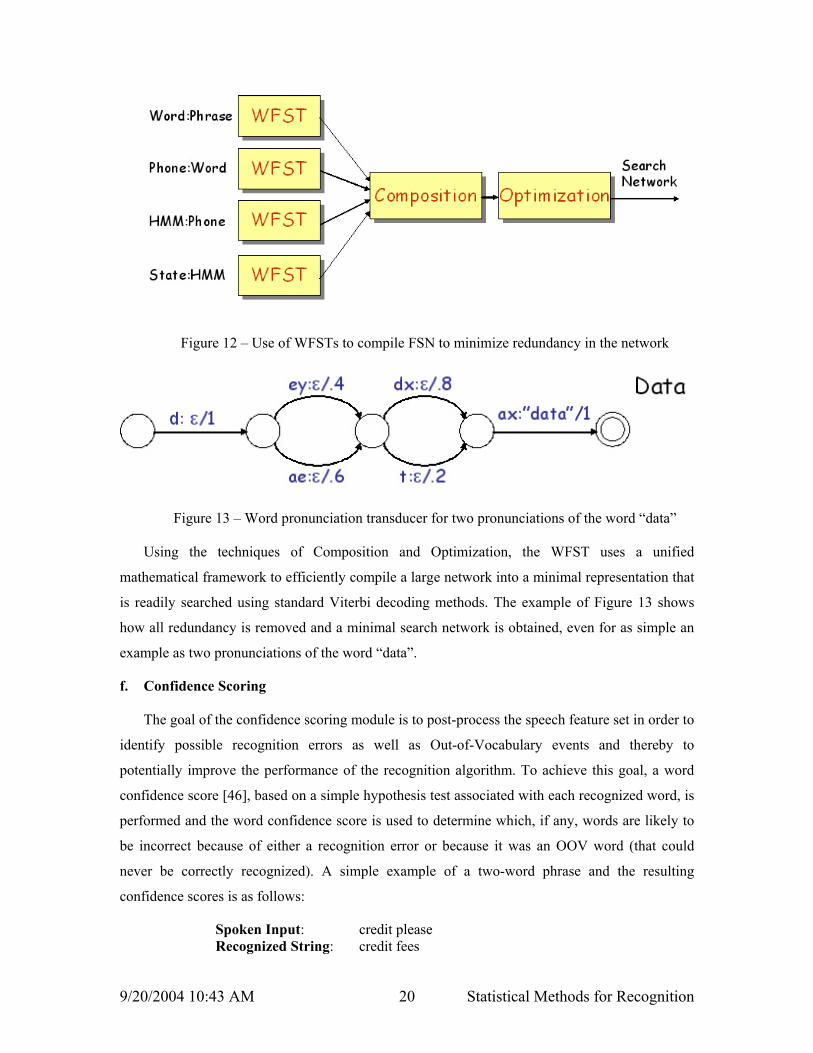
9/20/2004 10:43 AM 20 Statistical Methods for Recognition
Figure 12 – Use of WFSTs to compile FSN to minimize redundancy in the network
Figure 13 – Word pronunciation transducer for two pronunciations of the word “data”
Using the techniques of Composition and Optimization, the WFST uses a unified
mathematical framework to efficiently compile a large network into a minimal representation that
is readily searched using standard Viterbi decoding methods. The example of Figure 13 shows
how all redundancy is removed and a minimal search network is obtained, even for as simple an
example as two pronunciations of the word “data”.
f. Confidence Scoring
The goal of the confidence scoring module is to post-process the speech feature set in order to
identify possible recognition errors as well as Out-of-Vocabulary events and thereby to
potentially improve the performance of the recognition algorithm. To achieve this goal, a word
confidence score [46], based on a simple hypothesis test associated with each recognized word, is
performed and the word confidence score is used to determine which, if any, words are likely to
be incorrect because of either a recognition error or because it was an OOV word (that could
never be correctly recognized). A simple example of a two-word phrase and the resulting
confidence scores is as follows:
Spoken Input: credit please Recognized String: credit fees

9/20/2004 10:43 AM 21 Statistical Methods for Recognition
Confidence Scores: (0.9) (0.3) Based on the confidence scores, the recognition system would realize which word or words
are likely to be in error and take appropriate steps (in the ensuing dialog) to determine whether an
error had been made and how to fix it so that the dialog moves forward to the task goal in an
orderly and proper manner. (We will discuss how this happens in the discussion of Dialog
Management later in this article).
7. Simple Example of ASR System – Isolated Digit Recognition
To illustrate some of the ideas presented above, consider a simple isolated word speech
recognition system where the vocabulary is the set of 11 digits (“zero” to “nine” plus the word
“oh” as an alternative for “zero”) and the basic recognition unit is a whole word model. For each
of the 11 vocabulary words we must collect a training set with sufficient, say K, occurrences of
each spoken word so as to be able to train reliable and stable acoustic models (the HMMs) for
each word. Typically a value of K=5 is sufficient for a speaker-trained system (that is a
recognizer that works only for the speech of the speaker who trained the system). For a speaker-
independent recognizer, a significantly larger value of K is required to completely characterize
the variability in accents, speakers, transducers, environments etc. For a speaker-independent
system based on using only a single transducer (e.g., a telephone line input), and a carefully
controlled acoustic environment (low noise), reasonable values of K are on the order of 100 to
500 for training reliable word models and obtaining good recognition performance.
For implementing an isolated-word recognition system, we do the following:
1. for each word, v, in the vocabulary, we build a word-based HMM, vλ , i.e., we must
(re-)estimate the model parameters vλ that optimize the likelihood of the K training
vectors for the v-th word. This is the Training phase of the system.
2. for each unknown (newly spoken) test word which is to be recognized, we measure the
feature vectors (the observation sequence), ],,,[ 21 NX xxx L= (where each
observation vector, xi is the set of MFCCs and their first and second order derivatives),
we calculate model likelihoods, VvXP v ≤≤1),|( λ for each individual word model
(where V is 11 for the digits case), and then we select as the recognized word the word
whose model likelihood score is highest, i.e., )|(maxarg1
*v
VvXPv λ
≤≤= . This is the
Testing phase of the system.

9/20/2004 10:43 AM 22 Statistical Methods for Recognition
Figure 14 shows a block diagram of a simple HMM-based isolated word recognition system.
Figure 14 – HMM-based Isolated Word Recognizer
8. Performance of Speech Recognition Systems
A key issue in speech recognition (and understanding) system design is how to evaluate the
system performance. For simple recognition systems, such as the isolated word recognition
system described in the previous section, the performance is simply the word error rate of the
system. For more complex speech recognition tasks, such as for dictation applications, we must
take into account the three types of errors that can occur in recognition, namely word insertions
(recognizing more words than were actually spoken), word substitutions (recognizing an incorrect
word in place of the correctly spoken word), and word deletions (recognizing fewer words than
were actually spoken) [47]. Based on the criterion of equally weighting all three types of errors,
the conventional definition of word error rate for most speech recognition tasks is:
| |NI NS NDWER
W+ +
=
where NI is the number of word insertions, NS is the number of word substitutions, ND is the
number of word deletions, and |W| is the number of words in the sentence W being scored. Based

9/20/2004 10:43 AM 23 Statistical Methods for Recognition
on the above definition of word error rate, the performance of a range of speech recognition and
understanding systems is shown in Table 1 below.
Corpus Type of Speech Vocabulary Size
Word Error Rate
Connect Digit String (TI Database) Spontaneous 11 (0-9, oh) 0.3%
Connect Digit String (AT&T Mall Recordings) Spontaneous 11 (0-9, oh) 2.0%
Connected Digit String (AT&T HMIHY) Conversational 11 (0-9, oh) 5.0%
Resource Management (RM) Read Speech 1000 2.0%
Airline Travel Information System (ATIS) Spontaneous 2500 2.5%
North American Business (NAB & WSJ) Read Text 64,000 6.6%
Broadcast News Narrated News 210,000 ~15%
Switchboard Telephone Conversation 45,000 ~27%
Call-Home Telephone Conversation 28,000 ~35%
Table 1 – Word Error Rates for a Range of Speech Recognition Systems
It can be seen that for a small vocabulary (11 digits) the word error rates are very low (0.3%)
for a connected digit recognition task in a very clean environment (TI Database) [48], but we see
that the digit word error rate rises significantly (to 5.0%) for connected digit strings recorded in
the context of a conversation as part of a speech understanding system (HMIHY) [3]. We also see
that word error rates are fairly low for 1000-2500 word vocabulary tasks (RM [49] and ATIS
[40]) but increase significantly as the vocabulary size rises (6.6% for a 64,000 word NAB
vocabulary, and 13-17% for a 210,000 word Broadcast News vocabulary), as well as for more
colloquially spoken speech (Switchboard and Call-Home [50]) where the word error rates are
much higher than comparable tasks where the speech is more formally spoken.
Figure 15 illustrates the reduction in word error rate that has been achieved over time for
several of the tasks from Table 1 (as well as other tasks not covered in Table 1). It can be seen
that there is a steady and systematic decrease in word error rate (shown on a logarithmic scale)

9/20/2004 10:43 AM 24 Statistical Methods for Recognition
over time for every system that has been extensively studied. Hence it is generally believed that
virtually any (task-oriented) speech recognition system can achieve arbitrarily low error (over
time) if sufficient effort is put into finding appropriate techniques for reducing the word error
rate.
Figure 15 – Reductions in speech recognition word error rates over time for a range of task-
oriented systems [51]
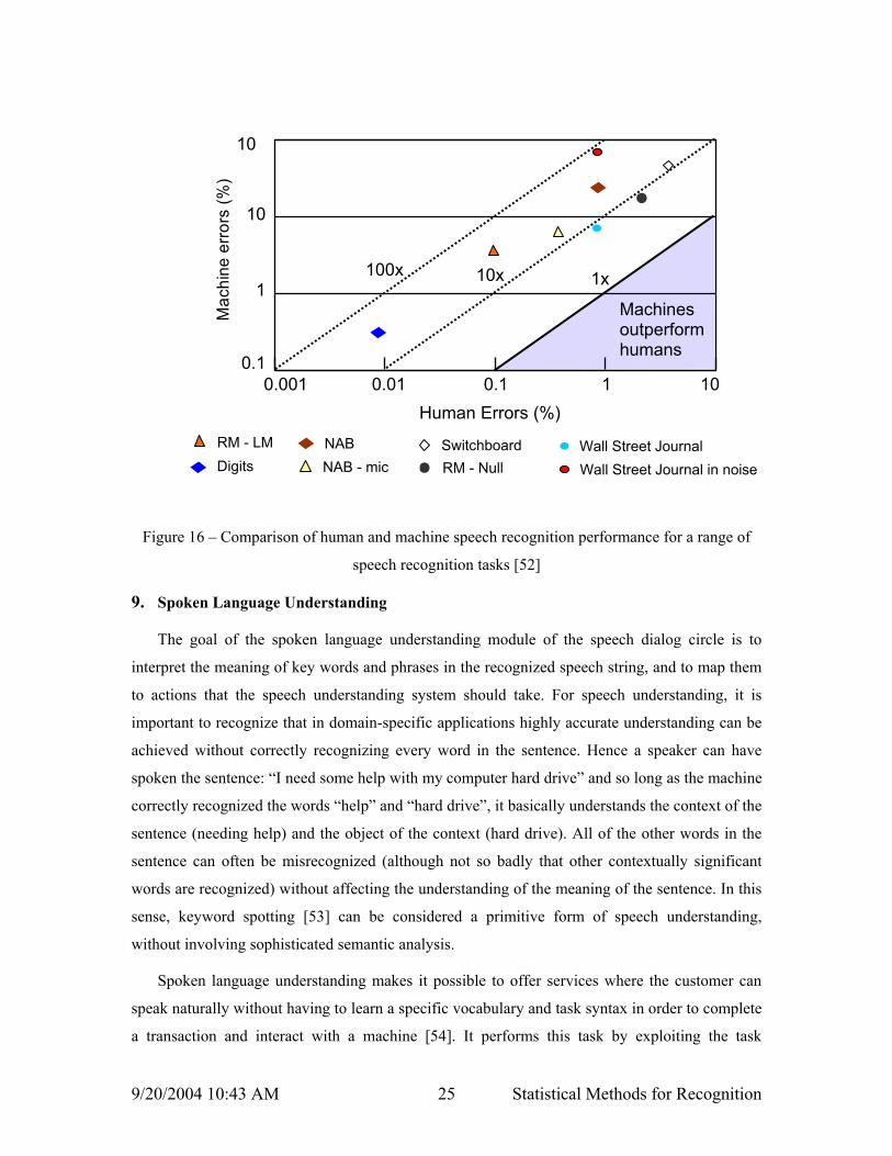
If one compares the best ASR performance for machines on any given task with human
performance (which often is hard to measure), the resulting comparison (as seen in Figure 16)
shows that machines outperform humans by factors of between 10 and 50; that is the machine
achieves word error rates that are larger by factors of from 10 to 50. Hence we still have a long
way to go before machines outperform humans on speech recognition tasks. However, one should
also note that under a certain condition an automatic speech recognition system could deliver a
better service than a human. One such example is the recognition of a long connected digit string,
such as a credit card’s 16-digit number, that is uttered all at once; a human listener would not be
able to memorize or jot down the spoken string without losing track of all the digits.
2001
20K, read10K, conversational
1K, read2K, spontaneous
64K, broadcast
99 9795939189 1987 0.1
10
100
1
Year
Wor
d Er
ror R
ate
(%)
digit
9/20/2004 10:43 AM 25 Statistical Methods for Recognition
Figure 16 – Comparison of human and machine speech recognition performance for a range of
speech recognition tasks [52]
9. Spoken Language Understanding
The goal of the spoken language understanding module of the speech dialog circle is to
interpret the meaning of key words and phrases in the recognized speech string, and to map them
to actions that the speech understanding system should take. For speech understanding, it is
important to recognize that in domain-specific applications highly accurate understanding can be
achieved without correctly recognizing every word in the sentence. Hence a speaker can have
spoken the sentence: “I need some help with my computer hard drive” and so long as the machine
correctly recognized the words “help” and “hard drive”, it basically understands the context of the
sentence (needing help) and the object of the context (hard drive). All of the other words in the
sentence can often be misrecognized (although not so badly that other contextually significant
words are recognized) without affecting the understanding of the meaning of the sentence. In this
sense, keyword spotting [53] can be considered a primitive form of speech understanding,
without involving sophisticated semantic analysis.
Spoken language understanding makes it possible to offer services where the customer can
speak naturally without having to learn a specific vocabulary and task syntax in order to complete
a transaction and interact with a machine [54]. It performs this task by exploiting the task
Machines outperform humans
0.001 0.01 0.1 1 100.1
1
10
10
Mac
hine
erro
rs (%
)
Human Errors (%)
100x 10x 1x
Digits NAB
RM - Null Wall Street Journal in noiseNAB - mic
RM - LM Switchboard Wall Street Journal
9/20/2004 10:43 AM 26 Statistical Methods for Recognition
grammar and task semantics to restrict the range of meanings associated with the recognized
word string, and by exploiting a pre-defined set of ‘salient’ words and phrases that map high
information word sequences to this restricted set of meanings. Spoken language understanding is
especially useful when the range of meanings is naturally restricted and easily cataloged so that a
Bayesian formulation can be used to optimally determine the meaning of the sentence from the
word sequence. This Bayesian approach utilizes the recognized sequence of words, W, and the
underlying meaning, C, to determine the probability of each possible meaning, given the word
sequence, namely:
( | ) ( | ) ( ) / ( )P C W P W C P C P W=
and then finding the best conceptual structure (meaning) using a combination of acoustic,
linguistic and semantic scores, namely:
* arg max ( | ) ( )C
C P W C P C=
This approach makes extensive use of the statistical relationship between the word sequence and
the intended meaning.
One of the most successful (commercial) speech understanding systems to date has been the
AT&T How May I Help You (HMIHY) task for customer care. For this task the customer dials
into an AT&T 800 number for help on tasks related to his or her long distance or local billing
account. The prompt to the customer is simply: “AT&T. How May I Help You?”. The customer
responds to this prompt with totally unconstrained fluent speech describing the reason for calling
the customer care help line. The system tries to recognize every spoken word (but invariably
makes a very high percentage of word errors), and then utilizes the Bayesian concept framework
to determine the meaning of the speech. Fortunately the potential meaning of the spoken input is
restricted to one of several possible outcomes, such as asking about Account Balances, or new
Calling Plans, or changes in Local service, or help for an Unrecognized Number, etc. Based on
this highly limited set of outcomes, the spoken language component determines which meaning is
most appropriate (or else decides not to make a decision but instead to defer the decision to the
next cycle of the dialog circle), and appropriately routes the call. The Dialog Manager, Spoken
Language Generation, and Text-to-Speech Modules complete the cycle based on the meaning
determined by the Spoken Language Understanding box. A simple characterization of the
HMIHY system is shown in Figure 17.

9/20/2004 10:43 AM 27 Statistical Methods for Recognition
Figure 17 – Conceptual representation of HMIHY system
The major challenge in spoken language understanding is to go beyond the simple
classification task of the HMIHY system (where the conceptual meaning is restricted to one of a
fixed, often small, set of choices) and to create a true concept and meaning understanding system.
10. Dialog Management, Spoken Language Generation and Text-to-Speech Synthesis
The goal of the dialog management module is to combine the meaning of the current input
with the interaction history with the user in order to decide what the next step in the interaction
should be. In this manner, the dialog management module makes viable fairly complex services
that require multiple exchanges between the system and the customer. Such dialog systems can
also handle user-initiated topic switching within the domain of the application.
The dialog management module is one of the most crucial steps in the speech dialog circle for
a successful transaction as it enables the customer to accomplish the desired task. The way in
which the dialog management module works is by exploiting models of dialog to determine the
most appropriate spoken text string to guide the dialog forward towards a clear and well
understood goal or system interaction. The computational models for dialog management include
both structure-based approaches (which models dialog as a pre-defined state transition network
that is followed from an initial goal state to a set of final goal states), or plan-based approaches
(which considers communication as executing a set of plans which are oriented toward goal
achievement).
The key tools of dialog strategy are the following:
• Confirmation: used to ascertain correctness of the recognized and understood utterances

9/20/2004 10:43 AM 28 Statistical Methods for Recognition
• Error recovery: used to get the dialog back on track after a user indicates that the system
has misunderstood something
• Reprompting: used when the system expected input but did not receive any input
• Completion: used to elicit missing input information from the user
• Constraining: used to reduce the scope of the request so that a reasonable amount of
information is retrieved, presented to the user, or otherwise acted upon
• Relaxation: used to increase the scope of the request when no information has been
retrieved
• Disambiguation: used to resolve inconsistent input from the user
• Greeting/Closing: used to maintain social protocol at the beginning and end of an
interaction
• Mixed initiative: allows users to manage the dialog flow
Although most of the tools of dialog strategy are straightforward and the conditions for their
use are fairly clear, the mixed initiative tool is perhaps the most interesting one as it enables a
user to manage the dialog and get it back on track whenever the user feels the need to take over
and lead the interactions with the machine. Figure 18 shows a simple chart that illustrates the two
extremes of mixed initiative for a simple operator services scenario. At the one extreme, where
the System manages the dialog totally, the system responses are simple declarative requests to
elicit information, as exemplified by the system command “Please say collect, calling card, third
number”. At the other extreme is User management of the dialog where the system responses are
open ended and the customer can freely respond to the system command “How may I help you?”.
Figure 18 – Illustration of mixed initiative for operator services scenario
Figure 19 illustrates some simple examples of the use of System Initiative, Mixed Initiative
and User Initiative for an airlines reservation task. It can be seen that System Initiative leads to
long dialogs (due to the limited information retrieval at each query) but the dialogs are relatively

9/20/2004 10:43 AM 29 Statistical Methods for Recognition
easy to design, whereas User Initiative leads to shorter dialogs (and hence a better user
experience) but the dialogs are more difficult to design.
Figure 19 – Examples of mixed initiative dialogs
Dialog management systems are evaluated based on the speed and accuracy of attaining a
well defined task goal, such as booking an airline reservation, renting a car, purchasing a stock, or
obtaining help with a service.
The spoken language generation module translates the action of the dialog manager into a
textual representation and the text-to-speech modules converts the textual representation into
natural sounding speech to be played to the user so as to initiate another round of dialog
discussion or to end the query (hopefully successfully).
11. User Interfaces and Multimodal Systems
The user interface for a speech communications system is defined by the performance of each of
the blocks in the speech dialog circle. A good user interface is essential to the success of any task-
oriented system, providing the following capabilities:
• It makes the application easy-to-use and robust to the kinds of confusion that arise in
human-machine communications by voice
• It keeps the conversation moving forward, even in periods of great uncertainty on the
parts of either the user or the machine

9/20/2004 10:43 AM 30 Statistical Methods for Recognition
• Although it cannot save a system with poor speech recognition or speech understanding
performance, it can make or break a system with excellent speech recognition and speech
understanding performance
Although we have primarily been concerned with speech recognition and understanding
interfaces to machines, there are times when a multimodal approach to human-machine
communications is both necessary and essential. The potential modalities that can work in concert
with speech include gesture and pointing devices (e.g., a mouse, keypad, stylus). The selection of
the most appropriate user interface mode (or combination of modes) depends on the device, the
task, the environment, and the user’s abilities and preferences. Hence when trying to identify
objects on a map (e.g., restaurants, locations of subway stations, historical sites), the use of a
pointing device (to indicate the area of interest) along with speech (to indicate the topic of
interest) often is a good user interface, especially for small computing devices like tablet PCs or
PDAs. Similarly when entering PDA-like information (e.g., appointments, reminders, dates,
times, etc.) onto a small handheld device, the use of a stylus to indicate the appropriate type of
information with voice filling in the data field is often the most natural way of entering such
information (especially as contrasted with using an artificial typing language such as graffiti for
Palm-like devices). Microsoft research has shown the efficacy of such a solution with the MIPad
(Multimodel Interactive Pad) demonstration, and they claim to have achieved double the
throughput for English using the multimodal interface over that achieved with just a pen stylus
and the graffiti language.
12. Summary
In this article we have outlined the major components of a modern speech recognition and
spoken language understanding system, as used within a voice dialog system. We have shown the
role of signal processing in creating a reliable feature set for the recognizer, and the role of
statistical methods in enabling the recognizer to recognize the words of the spoken input sentence
as well as the meaning associated with the recognized word sequence. We have shown how a
dialog manager utilizes the meaning accrued from the current as well as previous spoken inputs to
create an appropriate response (as well as potentially taking some appropriate actions) to the
customer request(s), and finally how the spoken language generation and text-to-speech synthesis
parts of the dialog complete the dialog circle by providing feedback to the user as to actions taken
and further information that is required to complete the transaction that is requested.
Although we have come a long way towards the vision of Hal, the machine that both
recognizes words reliably and understands their meaning almost flawlessly, we still have a long

9/20/2004 10:43 AM 31 Statistical Methods for Recognition
way to go before this vision is fully achieved. The major problem that must yet be tackled is
robustness of the recognizer and the language understanding system to variability in speakers,
accents, devices, and environments in which the speech is recorded. Systems that appear to work
almost flawlessly under laboratory conditions often fail miserably in noisy train or airplane
stations, when used with a cellphone or a speakerphone, when used in an automobile
environment, or when used in noisy offices. There are many ideas that have been advanced for
making speech recognition more robust, but to date none of these ideas has been able to fully
combat the degradation in performance that occurs under these non-ideal conditions.
Speech recognition and speech understanding systems have made their way into mainstream
applications and almost everybody has used a speech recognition device at one time or another.
They are widely used in telephony applications (operator services, customer care), in help desks,
in desktop dictation applications, and especially in office environments as an aid to digitizing
reports, memos, briefs, and other office information. As speech recognition and speech
understanding systems become more robust, they will find their way into cellphone and
automotive applications, as well as into small devices, providing a natural and intuitive way to
control the operation of these devices as well as to access and enter information.

9/20/2004 10:43 AM 32 Statistical Methods for Recognition
References
1. Cox, R. V., Kamm, C. A., Rabiner, L. R., Schroeter, J. and Wilpon, G. J., “Speech and language processing for next-millennium communications services,” Proc. of the IEEE, vol. 88, no. 8, August 2000, pp. 1314-1337.
2. Roe, D. B., Wilpon, J. G., Mikkilineni, P. and Prezas, D., ``AT&T's speech recognition in the telephone network,'' Speech Technology Mag., vol. 5, no. 3, Feb/March 1991, pp. 16-22.
3. Gorin, A. L., Parker, B. A., Sachs, R. M. and Wilpon, J. G., ``How may I help you?,'' Proc. Interactive Voice Technology for Telecommunications Applications (IVTTA), Oct. 1996, pp. 57-60.
4. Sugamura N., Hirokawa T., Sagayama S., and Furui S., Speech Processing Technologies and Telecommunications Applications at NTT, Proc. IVTTA 94, pp. 37-42, 1994.
5. Rabiner, L.R, Juang, B.H., and Lee, C.H., An Overview of Automatic Speech Recognition, in Automatic Speech & Speaker Recognition – Advanced Topics, Lee et.al. (ed.), p.1-30, Kluwer Academic, Norwell, Massachusetts, 1996.
6. Gauvain J-L., and Lamel L., Large Vocabulary Speech Recognition Based on Statistical Methods, inPattern Recognition in Speech & Language Processing, Chou and Juang (eds.), p. 149-189, CRC Press, New York, 2003.
7. Young, S.J., A Review of Large Vocabulary Continuous Speech Recognition, IEEE Signal Processing Magazine, 13(5):45-57, September 1996.
8. Rabiner, L.R., Wilpon, J.G., and Juang, B.H., A model-based connected-digit recognition system using either hidden Markov models or templates, Computer Speech & Language, Vol. 1, No. 2, pp.167-197, December 1986.
9. Jelinek, F., Statistical Methods for Speech Recognition, MIT Press, Cambridge, 1997.
10. Rosenfeld, R., Two Decades of Statistical Language Modeling: Where Do we Go From Here?, Proceedings of the IEEE, Special Issue on Spoken Language Processing, 88(8):1270-1278, August 2000.
11. Ney, H., The Use of A One Stage Dynamic Programming Algorithm for Connected Word Recognition, IEEE Trans. Acoustics, Speech and Signal Processing, ASSP-32(2):263-271, April 1984.
12. Paul, D.B., An Efficient A* Stack Decoder Algorithm for Continuous Speech Recognition with A Stochastic Language Model, Proceedings IEEE ICASSP-01, Salt Lake City, May 2001.
13. M. Mohri, Finite-State Transducers in Language and Speech Processing, Computational Linguistics, Vol. 23, No. 2, pp. 269-312, 1997.
14. Juang, B.H., Thomson, D., and Perdue, R.J., Deployable automatic speech recognition systems - advances and challenges," AT&T Technical Journal, Vol.74, No.2, 1995.
15. Kamm, C., & Helander, M., Design Issues for Interfaces Using Voice Input, In M. Helander, T. K. Landauer, & P. Prabhu (Eds)., Handbook of human-computer interaction, pp. 1043-1059, Elsevier, Amsterdam, 1997.
16. ISCA Archive, Disfluency in Spontaneous Speech (DiSS'01), ISCA Tutorial and Research Workshop (ITRW), Edinburgh, Scotland, UK, August 29-31, 2001, http://www.isca-speech.org/archive/diss_01.

9/20/2004 10:43 AM 33 Statistical Methods for Recognition
17. Davis, S. and Mermelstein, P., Comparison of Parametric Representations of Monosyllabic Word Recognition in Continuously Spoken Sentences, IEEE Trans. Acoust. Speech Signal Processing, 28(4):357-366, 1980.
18. Furui, S., Comparison of Speaker Recognition Methods using Static Features and Dynamic Features, IEEE Trans. Acoust. Speech Signal Processing, ASSP-29, pp.342-350, 1981.
19. Rabiner, L.R. and Gold, B., Theory and Applications of Digital Signal Processing, Prentice-Hall, Englewood Cliffs, NJ, 1975.
20. Atal, B.S. and Hanauer, S.L., Speech Analysis and Synthesis by Linear Prediction of the Speech Wave, J. Acoust. Soc. Am., 50(2):637:655, August 1971.
21. Markel, J.D. and Gray, A.H., Jr., Linear Prediction of Speech, Springer-Verlag, 1976.
22. Rahim, M., Juang, B.H., Signal bias removal by maximum likelihood estimation for robust telephone speech recognition," IEEE Trans. Speech & Audio Processing, V.4, No.1, pp.19-30, January 1996.
23. Levinson, S.E., Rabiner L.R., and Sondhi, M.M., An Introduction to the Application of the Theory of Probabilistic Functions of a Markov Process to Automatic Speech Recognition, Bell Syst. Tech. J., Vol. 62, No. 4, pp. 1035-1074, April 1983.
24. J. D. Ferguson, Hidden Markov Analysis: An Introduction, in Hidden Markov Models for Speech, Institute for Defense Analyses, Princeton, NJ 1980.
25. Rabiner, L.R., A Tutorial on Hidden Markov Models and Selected Applications in Speech Recognition, Proceedings of the IEEE, 77(2):257-286, 1989.
26. Rabiner, L.R., and Juang, B.H., An Introduction to Hidden Markov Models, IEEE Signal Processing Magazine, 1985.
27. Juang, B.H., Levinson, S.E., and Sondhi, M.M, Maximum Likelihood Estimation for Multivariate Mixture Observations of Markov Chains, IEEE Trans. Information Theory, Vol. It-32, No. 2, pp. 307-309, March 1986.
28. Juang, B.H., Maximum Likelihood Estimation for Mixture Multivariate Stochastic Observations of Markov Chains, AT&T Tech. J., Vol. 64, No. 6, pp. 1235-1249, July-Aug. 1985.
29. Baum, L.E., An Inequality and Associated Maximization Technique in Statistical Estimation for Probabilistic Functions of Markov Processes, Inequalities, Vol. 3, pp. 1-8, 1972.
30. Baum, L.E., Petri, T., Soules, G., and Weiss, N., A maximization technique occurring in the statistical Analysis of probabilistic functions of Markov chains, Ann. Math. Stat., 41:164:171, 1970.
31. Lee, K.-F., The Development of the Sphinx System, Kluwer, 1989.
32. Lee, C. H., Juang, B. H., Soong, F. K. and Rabiner, L. R., Word Recognition Using Whole Word and Subword Models, Conference Record 1989 IEEE International Conference on Acoustics, Speech, and Signal Processing, Paper S 12.2, pp. 683-686, May 1989.
33. Jurafsky, D. S., & Martin, J.H., Speech and Language Processing. Prentice Hall, Inc., Englewood, N.J., 2000.

9/20/2004 10:43 AM 34 Statistical Methods for Recognition
34. Riley, M.D., et al., Stochastic Pronunciation Modeling from Hnad-Labelled Phonetic Corpora, Speech Communication, 29(2-4) :209-224, November 1999.
35. Jelinek, F., Mercer, R.L., and Roukos, S., Principles of lexical language modeling for speech recognition, in Advances in Speech Signal Processing, Furui & Sondhi (eds.), p.651-699, Mercer Dekker, New York, 1991.
36. Bahl, L.R., Jelinek, F., and Mercer, R.L., A Maximum Likelihood Approach to Continuous Speech Recognition, IEEE Trans. Pattern Analysis & Machine Intelligence, PAMI-5(2):179-190, March 1983.
37. Nadas, A., On Turing's formula for word probabilities, IEEE Transactions on Acoustics, Speech, and Signal Processing, Vol. ASSP-33(6), 1414-1416, 1985.
38. Roukos, Salim, Language Representation, in Survey of the State of the Art in Human Language Technology, Giovanni Battista Varile and Antonio Zampolli (eds.), Cambridge University Express, 1998.
39. Cover, T. and Thomas, J., Elements of Information Theory, Wiley Series in Telecommunications, John Wiley and Sons, 1991.
40. Ward, W., Evaluation of the CMU ATIS System, Proceedings of the DARPA Speech and Natural Language Workshop, February 19-22, 1991, pp. 101-105, 1991.
41. Price, P., Evaluation of spoken language systems: the ATIS domain, in Proceedings of the Third DARPA SLS Workshop, P. Price, Ed. Morgan Kaufmann, June 1990.
42. Paul, D.B. and Baker, J.M., The design for the Wall Street Journal-based CSR corpus, in Proceedings of the DARPA SLS Workshop. February 1992.
43. Kawahara, T. and Lee, C.H., Flexible speech understanding based on combined key-phrase detection and verification, IEEE Trans. Speech & Audio Processing, T-SA, vol.6, no.6, pp.558-568, November 1998.
44. Forney, D., The Viterbi Algorithm, Proceedings IEEE, 61:268-278, March 1973.
45. Bellman, R., Dynamic Programming. Princeton University Press, Boston, 1957.
46. Rahim M, Lee C.-H., Juang B.-H., Discriminative Utterance Verification for Connected Digit Recognition, IEEE Transactions on Speech and Audio Processing, vol. 5, no. 3, pp. 266-277, May 1997.
47. Pallett, D. and Fiscus, J. 1996 preliminary broadcast news benchmark tests. In DARPA 1997 speech recognition workshop, 1997.
48. Leonard, R. G., A database for speaker-independent digit recognition, Proceedings of ICASSP, IEEE International Conference on Acoustics, Speech and Signal Processing, pp. 42.11.1-42.11.4., 1984.
49. Linguistic Data Consortium, LDC Catalog Resource Management RM 2 2.0, http://wave.ldc.upenn.edu/Catalog/CatalogEntry.jsp?catalogId=LDC93S3C, 1992-2000.
50. Godfrey, J.J., Holliman, E.C., and McDaniel, J., SWITCHBOARD: Telephone speech corpus for research and development. In Proceedings of the IEEE Conference on Acoustics, Speech and Signal Processing, vol. I, pp. 517–520, San Francisco, 1992.
51. Pallett, D.S., et al, 1994 Benchmark Tests for the ARPA Spoken Language Program, Proc. Of the 1995 ARPA Human Language Technology Workshop, pp. 5-36, 1995.

9/20/2004 10:43 AM 35 Statistical Methods for Recognition
52. Lippman, R.P., Speech recognition by machines and humans, Speech Communication, vol. 22, no. 1, pp 1-15. 1997.
53. Wilpon, J. G., Rabiner, L. R., Lee, C-H. and Goldman, E., Automatic recognition of keywords in unconstrained speech using hidden Markov models, IEEE Trans. on Acous. Speech & Sig. Proc., vol. 38, no. 11, Nov. 1990, pp. 1870-1878.
54. Juang, B.H., and Furui, S., Automatic recognition and understanding of spoken language – a first step towards natural human-machine communication,” Proceedings of the IEEE, August 2000.