912 IEEE TRANSACTIONS ON PATTERN ANALYSIS AND...

912 IEEE TRANSACTIONS ON PATTERN ANALYSIS AND MACHINE INTELLIGENCE, VOL. 18, NO. 9, SEPTEMBER 1996

Structure Learning of Bayesian Networks by Genetic Algorithms:

Performance Analysis of Control Parameters Pedro Larrafiaga, Mike1 Poza, Yosu Yurramendi, Roberto H. Murga, and Cindy M.H. Kuijpers

Abstract-We present a new approach to structure learning in the field of Bayesian networks: We tackle the problem of the search for the best Bayesian network structure, given a database of cases, using the genetic algorithm philosophy for searching among alternative structures. We start by assuming an ordering between the nodes of the network structures. This assumption is necessary to guarantee that the networks that are created by the genetic algorithms are legal Bayesian network structures. Next, we release the ordering assumption by using a “repair operator” which converts illegal structures into legal ones. We present empirical results and analyze them statistically. The best results are obtained with an elitist genetic algorithm that contains a local optimizer.

Index Terms-Bayesian network, genetic algorithm, structure learning, combinatorial optimization, performance analysis

1 INTRODUCTION AYESIAN networks (BNs) have become popular over the last few years within the AI probability and uncertainty

community as a method of reasoning under uncertainty. From an informal perspective, BNs are directed acyclic graphs (DAGs), where the nodes are random variables and where the arcs specify the indepen.dence assumptions between these variables. After construction, a BN constitutes an efficient device for performing probabilistic inference.

The problem of searching the BN that best reflects the dependence relations in a database of cases is a difficult one because of the large number of possible DAG structures, given even a small number of nodes to connect. In this paper, we present a method for solving this problem of the structure learning of BNs from a database of cases based on genetic algorithms.

The structure of the paper is as follows. In the next section, we introduce the Bayesian networks and we describe the problem of the search of such a network from a database of cases. A brief introduction on genetic algorithms is given in Section 3. In Section 4, we show how genetic algorithms can be used for tackling the problem of the structure learning of BNs. We describe two different approaches, namely with and without assuming an ordering between the nodes of the network. In the latter approach, the offspring constructed by the genetic algorithm are not necessarily BN structures, they may have to be repaired. In both approaches we use a Bayesian approach to measure the fitness of the structures. Empirical results obtained with simulations of the ASIA and ALARM networks are pre-

l The authors ure with fke Department of Computer Science and Artificial Intelligence, University of fke Basque Country, P.O. Box 649, E-20050 San Sebastidn, Spain. E-mail: lccplamup, ccpyumej, ccbmugar, ccbkuhc}@si.eku.es.

Manuscript received Mar. 16,1995; revised Mar. 27,1996. Recommended for acceptance by H.R. Keskavan. For information on obtaining reprints of this article, please send e-mail to: [email protected], and reference IEEECS Log Number I’96041

sented in Section 5. Finally, in Section 6, we conclude the work and give some directions for future research.

2 BAYESIAN NETWORKS AND STRUCTURE LEARNING Bayesian networks and associated schemes constitute a probabilistic f ramework for reasoning under uncertainty that in recent years has gained popularity in the community of artificial intelligence [l], [2], [3].

From an informal perspective, Bayesian networks are directed acyclic graphs (DAGs), where the nodes are random variables, and the arcs specify the independence assumptions that must be held between the random variables.

To specify the probability distribution of a BN, one must give prior probabilities for all root nodes (nodes with no predecessors) and conditional probabilities for all other nodes, given all possible combinations of their direct predecessors. These numbers in conjunction with the DAG, specify the BN completely. The joint probability of any particu- lar instantiation of all n variables in a BN can be calculated as follows:

P(q, ..‘I XJ = fp(xz I Xi) i=l

where xi represents the instantiation of the variable X, and ni represents the instantiation of the parents of Xi.

Once the network is constructed it constitutes an efficient device to perform probabilistic inference. Neverthe- less, the problem of building such a network remains. The structure and conditional probabilities necessary for char- acterizing the network can be provided either externally by experts or from direct empirical observations. The learning task in a BN can be separated into two subtasks, structure learning, that is to identify the topology of the network, and parameter learning, the numerical parameters (conditional probabilities) for a given network topology.

0162~8828/96$05.00 01996 IEEE

LARRAAAGA ET AL.: STRUCTURE LEARNING OF BAYESIAN NETWORKS BY GENETIC ALGORITHMS 913

Our work focuses upon structure learning rather than upon parameter learning. However, for complete BN construction it is also necessary to estimate the parameters. Previous research in structure learning of BNs has already been carried out. Some authors [4], [5], 161 have worked on inducing the structure of trees or polytrees from a database of cases. The more relevant works on structure learning on multiply connected networks have been developed in [7], 181, t91, [lO I, ill], t121, [131, [141, t151, [Id, 1171, 1181, [191, POI, LXl,t221, P-31, D41, MI, P261.

A frequently used procedure for BN network structure construction from data is the K2 algorithm of Cooper and Herskovits [9]. This algorithm (see Fig. 1) searches, given a database D for the BN structure Bs* with maximal P(Bs,D), where P(B,,D) is as described in the following theorem proved in [9].

Algorithm K2

INPUT: A set of n nodes, an ordering on the nodes, an up- per bound u on the number of parents a node may have, and a database D containing m cases. OUTPUT: For each node, a printout of the parents of the node. BE GIN K2

FOR i:=lTOnDO BEG IN

r& := 0; Pold := g(i, HJ: OKToProceed := TRUE WHI LE OKToProceed AND I Q I < u DO

BEG IN Let Z be the node in Pred(XJ - II, that

maximizes g(i, Q U {Zl); P,,, := g(i, I& U Kl); IF P,,, > Pold THEN

BEG IN POld := p,,,; q := I-& u {Z)

END ELSE OKToProceed := FALSE;

END; WRITE(‘Node:,’ Xi, ‘Parents of this node:,’ IIJ

END; END K2.

Fig. 1. The K2 algorithm.

THEOREM. Let Z be a set of n discrete variables, where a variable Xi in Z has ri possible value assignments: (vi,, . . . , vi,, ) . Let D be a database of m cases, where each case contains a value assignment for each variable in Z. Let Bs denote a belief network structure containing just the variables in Z, and B, the conditional probabilities. Each variable Xi in Bs has a set of parents, which are represented with a list of

variables I& Let Wlj denote the jth unique instantiation of

lIi relative to D. Suppose there are 9i such unique instan- tiations of I&. Define Nijk to be the number of cases in D in which variable Xi has the value Vik and I& is instantiated as

wii. Let Nq = czz, Niik . If given a BN model, the cases

occur independently and the density function f(BD I B,) is uniform, then it follows that

P(B,,D) = P(Bs)fifi (‘-‘)! fiNqk! i=l jz1 (NV + q - 1) ! k=l

The K2 algorithm assumes that an ordering on the variables is available and that, a priori, all structures are equally likely. It searches, for every node, the set of parent nodes that maximizes the following function:

8(i’ni) = fi tl; -l)! ) nN,!. N ,, +y, -1 I ‘I ’

‘_ .k 1

K2 is a greedy heuristic. It starts by assuming that a node lacks parents, after which in every step it adds incrementally that parent whose addition most increases the probability of the resulting structure. K2 stops adding parents to the nodes when the addition of a single parent can not increase the probability. Obviously, this approach does not guarantee to obtain the structure with the highest probability.

A possible improvement of K2 could be the determination of the best combination of at most u parent nodes in which case the number of searches to be carried out for a node j

wouldincreasefromnyzl(n-j-i) to~~~,(“-/-‘).

In Section 4, we present a genetic search algorithm for BN structures that for the evaluation of these structures uses the same metric as K2. We start by maintaining the same ordering restiction on the variables as K2, after which this restriction is released.

3 GENETIC ALGORITHMS Recently five approaches of heuristic search have emerged for solutions to combinatorial complex problems: evolutionary algorithms, neural networks, simulated annealing, tabu search, and target analysis. The first two-evolutionary algorithms and neural networks-are inspired by principles derived from biological sciences; and simulated annealing de- rives from physical science, notably the second law of ther- modynamics. Tabu search and target analysis stem from the general tenets of intelligent problem-solving.

Evolutionary algorithms are probabilistic search algorithms which simulate natural evolution. They were proposed about 30 years ago [271, [281. Their application to combinatorial optimization problems, however, has only recently become an actual research topic. Roughly speaking three different types of evolutionary algorithms exist: genetic algorithms [29], 1301, [31], evolutionary programming [32], and evolution strategies [33]. In this paper we consider the genetic algorithms (GAS). GAS are search algorithms based on the mechanics of natural selection and natural genetics. They combine survival of the fittest among string


structures with a structured yet randomized information exchange to form a search algorithm that under certain conditions evolves to the optimum with probability arbi- trarily close to 1 [341,1351, [361,1371, 1381.

In GAS the search space of a problem is represented as a collection of individuals. The individuals are represented by character strings, which are often referred to as chromo- somes. The purpose of the use of a GA is to find the individual from the search space with the best “genetic mate- rial.” The quality of an individual is measured with an objective function. The part of the search space to be exam- ined is called the population.

Roughly, a GA works as follows: First, the initial population is chosen, and the quality of each of its individuals is determined. Next, in every iteration parents are selected from the population. These parents produce children, which are added to the population. For all newly created individuals of the resulting population a probability near zero exits that they “mutate,” i.e., they change their he- reditary distinctions. After that, some individuals are re- moved from the population according to a selection criterion in order to reduce the population to its initial size. One iteration of the algorithm is referred to as a generation.

The operators which define the child production process and the mutation process are called the crossover operator and the mutation operator respectively. Both operators are applied with different probabilities named the crossover probability and the mutation probability. Mutation and crossover play different roles in the GA. Mutation is needed to explore new states and helps the algorithm to avoid local optima. Crossover should increase the average quality of the population. By choosing adequate crossover and mutation operators as well as an appropriate reduction mechanism, the probability that the GA results in a near-optimal solution in a reasonable number of iterations increases.

The pseudocode of an abstract genetic algorithm (AGA), is shown in Fig. 2.

Definitions and details of operators related to GAS are defined in Appendix A.

begin AGA Make initial population at random WHILE NOT stop DO

BEGIN Select parents from the population. Produce children from the selected parents. Mutate the individuals. Entend the population by adding the children to it. Xeduce the extended population. END

Output the best individual found. end AGA

Fig. 2. The pseudocode of the abstract genetic algorithm.

4 GENETIC ALGORITHMS IN THE STRUCTURE LEARNING OF BAYESIAN NETWORKS

4.1 Notation and Representation Our approach on structure learning in the framework of Bayesian networks is based on genetic algorithms. Denot- ing with D the set of BN structures for a fixed domain with n variables, and the alphabet S being {O,l 1, a Bayesian network structure can be represented by an n x n connectivity matrix C, where its elements, cij, verify:

1 % =

if i is a parent of i, 0 otherwise.

In our genetic approach, we represent an individual of the population by string:

q,cz* . C,,C$** . c,* . ClnC2n . . c,,.

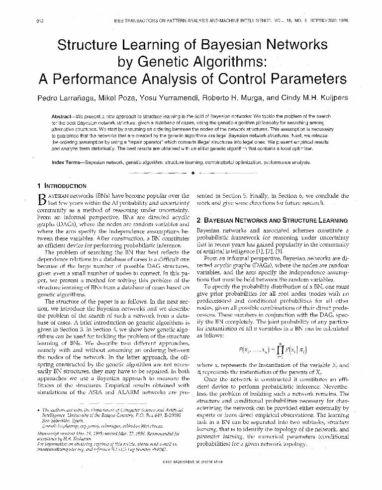
With this representation in mind, we will show how the crossover and mutation operators work, by using simple examples EXAMPLE 1. Consider a domain of three variables on which

the two BN structures of Fig. 3 are defined. The connectivity matrices that correspond to the network structures are, respectively,

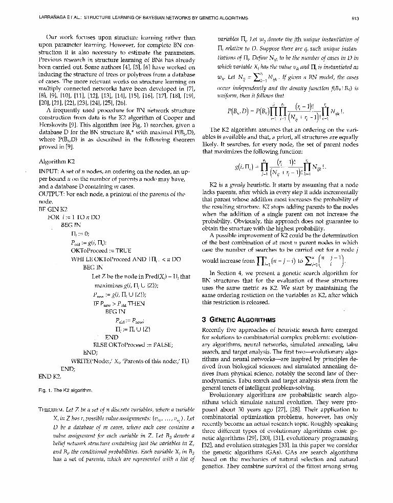
Using the above described representation, the networks are represented by the strings: 001001000 and 000000110. Suppose now that the two network structures are selected to crossover and that the crossover point is chosen between the sixth and the seventh bit. This gives the offspring strings 001001110 and 000000000. Hence, the created offspring structures are the ones presented in Fig. 4.

Fig. 3. The parent structures of Example 1,

Xl x2

::.i:;

0 x3

x3 @ @

Fig. 4. Crossover does not always result in legal structures.

LARRAfiAGA ET AL.: STRUCTURE LEARNING OF BAYESIAN NETWORKS BY GENETIC ALGORITHMS 915

We see that the offspring structures do not correspond to DAGs. We say that the one point crossover operator is not a closed operator.

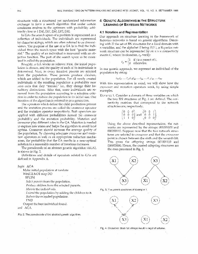
EXAMPLE 2. Consider the DAG of Fig. 5a. It is represented by the string 010001000. Suppose that the seventh bit is altered by mutation. This gives the string 010001100, which corresponds with to cyclic graph of Fig. 5b. We observe that the mutation operator is not a closed operator either.

(4

Fig. 5. Mutation is not a closed operator.

@I

4.2 With Ordering Between the Nodes In the previously mentioned methods to tackle the structure learning of BN structures, most often an ordering between the variables of the BN is assumed. This means that a node Xi can only have node Xj as a parent node if in the ordering node X1 comes before node Xi. It is easy to verify that in case an ordering is assumed, the connectivity matrices of the network structures are triangulated and that therefore the genetic operators are closed operators. In this case the string’s length used to represent a BN structure with n

nodes is ’ 0

2 , instead of PZ’ of the general case. Under the

ordering assumption the cardinality of the search space is

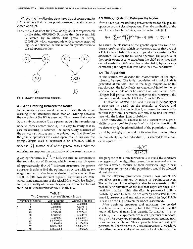
given by the formula 2(‘). In [39], the authors demonstrate that for a domain of 10 nodes, which means a search space of approximately 35 x 10 l2 different structures, the genetic approach is able to find the optimum structure with an average number of structures evaluated that is smaller than 4,000. In [40], two different types of algorithms are compared using simulations of the ALARM network. See Table 1 for the cardinality of the search space for different values of n, where n is the number of nodes in the BN.

TABLE 1 THE CARDINALITY OF THE SEARCH SPACE

number of nodes With ordering 5 1.024e03 8 2.684e08

Without ordering 2.928e04 7.837ell 4.175e18 2.377e41 2.344e72

2.659elll 2.714e158 2.118e213 3.008e237 1.124e276

4.3 Without Ordering Between the Nodes If we do not assume ordering between the nodes, the genetic operators are not closed operators. Then the cardinality of the search space (see Table 1) is given by the formula 1411:

f(n) = 2 (-*)i+1(;)2”“-i~f(n - i), f(0) = 1, f(1) = 1. i=l

To assure the closeness of the genetic operators we introduce a repair operator, which converts structures that are not a DAG into a DAG. This repair operator is inserted in the algorithm, just after the mutation operator. The objective of the repair operator is to transform the child structures that do not verify the DAG conditions into DAGs, by randomly eliminating the edges that invalidate the DAG conditions.

4.4 The Algorithm In this section, we describe the characteristics of the algorithms to be used. The initial population of a individuals is generated at random. Due to the huge magnitude of the search space, the individuals are created subjected to the restriction that a node never has more than four parent nodes. Hiiffgen 1421 proves that even subject to this restriction, the problem of model search of BN structures is NP-hard.

The objective function to be used to evaluate the quality of a structure, is based on the formula of Cooper and Herskovits, described in Section 2, expressed in terms of the natural logarithm. Therefore, our aim is to find the structure with the highest joint probability.

Each individual is selected to be a parent with a probability proportional to the rank of its objective function. If we denote by I/ the jth individual of the population at time t, and by rank(g(l:)) the rank of its objective function, then

the probability pj,* that individual I/ is selected to be a parent is equal to

The purpose of this transformation is to avoid the premature convergence of the algorithm caused by superindividuals, individuals which, because of their extremely large fitness with respect to the rest of the population, would be selected almost always.

In the offspring production process, two parent BN structures are recombined by means of l-point crossover. The mutation of the offspring structures consists of the probabilistic alteration of the bits that represent their connectivity matrices. This alteration is performed with a probability near to zero. As we already remarked in Sec- tion 4.2, crossover and mutation only result in legal DAGs in case an ordering between the nodes is assumed.

After applying crossover and mutation, the created structures do not necessarily fulfill the restriction that the nodes all have at most four parents. To maintain this restriction, in a first approach, we select q,parents at random, (0 < 4 < 4), for every node from the parent nodes resulting from crossover and mutation. This approach, however, will give poor results. Therefore, we try a second approach in which we hybridize the genetic algorithm, with a local optimizer. This


optimizer selects the best subset of at most four parent nodes for each node in a network structure. The process of generating child structures and the application of the local optimizer, is repeated in every iteration of the algorithm.

Once the offspring are converted into DAGs in which the nodes never have more than four parents, they are added to the population, after which this population is reduced to its original size. This reduction is carried out following two different criteria to which we will refer to as the elitist (of degree 1) reduction criterion and the simple reduction criterion. Using the former criterion, the population in the next iteration consists of the ;1 best structures (among parents and offspring) in the current iteration. With the latter criterion, the children in the current iteration constitute the population in the next iteration.

We decide to stop the algorithms when either 10,000 structures have been evaluated or when in 1,000 successive evaluations, the value of the objective function of the best structure corresponds with the average value of the objective function.

The algorithm uses the following parameters:

Population size ;1, in the next section we will present results of experiments carried out with ;1= 10 and it = 50.

Crossover probability pc, we choose pC = 0.5 and pC = 0.9.

Mutation rate pm, we will consider p, = 0.1 and pm = 0.01.

Reduction criterion, we use the simple reduction criterion as well as the elitist reduction criterion.

Ordering restriction, experiments are done with and without assuming ordering between the nodes. The absence of the ordering assumption implies the neces- sity of the repair operator.

Hybridization, we carry out experiments with and without local optimizer. When the local optimizer is not used the excess parent nodes are deleted at random. If the local optimizer is used, for each node the best subset of at most four parents is chosen-the subset which maximizes the posterior probability-from the set of its parent nodes.

5 RESULTS OF THE EXPERIMENTS

5.1 Introduction In this section we present the empirical results obtained. The different steps to evaluate the behavior of the genetic algorithms considered, have been the following:

l Step 1: Determinate a BN (structure + conditional probabilities) and simulate it, obtaining a database of cases D, which must reflect the conditional independence relations between the variables.

l Step 2: Using the approach based on genetic algorithms try to obtain the BN structure B,*, which maximizes the probability P(D I B,).

0 Step 3: Evaluate the fitness of the solutions found.

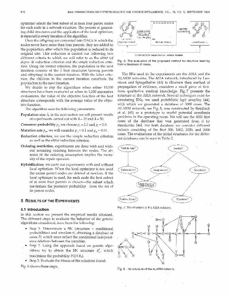
Fig. 6 shows these steps.

Bay&m nework database of cases

Fig. 6. The evaluation of the proposed method for structure learning from a database of cases.

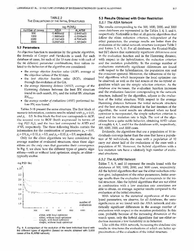
The BNs used in the experiments are the ASIA and the ALARM networks. The ASIA network, introduced by Lau- ritzen and Spiegelhalter [43] to illustrate their method of propagation of evidence, considers a small piece of ficti- tious qualitative medical knowledge. Fig. 7 presents the structure of the ASIA network. Several techniques exist for simulating BNs, we used probabilistic logic sampling [44], with which we generated a database of 3000 cases. The ALARM network, see Fig. 8, was constructed by Beinlinch et al. [45] as a prototype to model potential anesthesia problems in the operating room. We will use the 3000 first cases of the database that was generated from it by Herskovits [46]. For both database we consider different subsets consisting of the first 500, 1000, 2000, and 3000 cases. The evaluations of the initial structures for the different databases can be seen in Table 2.

Fig. 7. The structure of the ASIA network.

Fig. 8. The structure of the ALARM network.

LARRAI;IAGA ET AL.: STRUCTURE LEARNING OF BAYESIAN NETWORKS BY GENETIC ALGORITHMS

TABLE 2 THE EVALUATIONS OF THE INITIAL STRUCTURES

I 4

5.2 Parameters As objective function to maximize by the genetic algorithm, the formula of Cooper and Herskovits is used. For each database of cases, for each of the 10 runs done with each of the 64 different parameter combinations, four values related to the behavior of the algorithm are considered:

l the average objective function value (AOF), average of the objective values of the 10 runs.

l the best objective function value (BOF), obtained through the evolution of the GA.

l the average Hamming distance (AHD), average of the Hamming distance between the best BN structure found in each search, BNf, and the initial BN structure BNjnitial.

l the average number of evaluations CANE) performed before BNr was found.

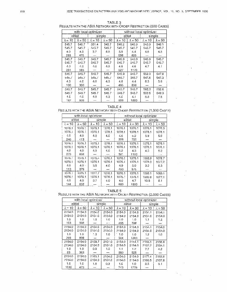
Tables 3-18 present the same structure. The first block of numeric information, contains results related with p, = 0.01, and pc = 0.5. In this block the first row corresponds to AOF, the second row to BOF (both expressed in terms of -log P(D I Bs)), and the two last correspond to AHD and ANE, respectively. The three following blocks contain the information for the combination of parameters: p, = 0.01, pc = 0.9; pm = 0.10, pc = 0.5, and p, = 0.10, pc = 0.9, respectively.

Only for the elitist algorithms we have considered the average number of evaluated structures, since these algorithms are the only ones that guarantee their convergence. In Fig. 9, we show how the different types of genetic algorithms-with or without local optimizer, simple, or elitist- typically evolve.

-log P(D I Bs)

x lo41

1.2 --

1.0 -- number of evaluations

I 200 400 600 800 1000

- elitist, with local optimizer . elitist, without local optimizer

- simple, with local optimizer simple, without local optimizer

Fig. 9. A comparison of the evolution of the best individual found with the different types of algorithm (based on results obtained with 3,000 cases of the ALARM network).

5.3 Results Obtained with Order Restriction 5.3.1 The ASIA Network The results corresponding to the 500, 1000, 2000,

917

and 3000 cases databases are represented in the Tables 3, 4, 5, and 6, respectively. Noticeable is that of all genetic algorithms that follow the elitist reduction criterion, independent of the other parameters, the average results are better than the evaluation of the initial network structure (compare Table 2 and Tables 3, 4, 5, 6). For all databases, the Kruskal-Wallis test [471 shows that statistically significant differences exist in the evaluation function and in the Hamming distance, with respect to the hybridization, the reduction criterion and the mutation probability. In the average number of evaluations statistically significant differences are found with respect to the hybridization, the population size and the crossover operator. Moreover, the robustness of the hybrid algorithms which incorporate the local optimizer can be observed, as well as the bad results of the no-hybrid algorithms which use the simple selection criterion. As the database size increases, the evaluation function increases and the evaluation function corresponding to the network structure, induced by the algorithm, adjusts to the evaluation of the initial structure. With respect to the average Hamming distance between the initial network structure and the best structures obtained in the last iteration of the algorithm, the worst results are obtained when no local optimizer is incorporated, the simple reduction criterion is used and the mutation rate is high. The rest of the algorithms have a quite stable behavior, obtaining AHD values of roughly 4,4,1, and 0 for the databases with, respectively, 500,1000,2000, and 3000 cases.

Evidently, the algorithms that use a population of 10 individuals converge faster than the ones that have a population of 50 individuals, the ones with a population of 10 carry out about half of the evaluations of the ones with a population of 50. Moreover, the hybrid algorithms with a low mutation rate have a relatively high number of evaluated structures.

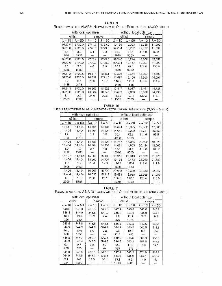
5.3.2 The ALARM Network Tables 7, 8, 9, and 10 represent the results found with the databases of 500, 1000, 2000, and 3000 cases, respectively. All the hybrid algorithms that use the elitist reduction criterion give, independent of the other parameters, better average results than the evaluation that corresponds to the initial structure. Also the hybrid algorithms that are not elitist in combination with a low mutation rate sometimes are able to obtain, on average, superior results compared to the evaluation of the initial structure.

With relation to the statistical significance of the analyzed parameters, we observe, for all databases, the same significances as we found with the ASIA network and statistically significant differences in the average number of evaluations with respect to the mutation probability. In this case, probably because of the increasing dimension of the search space, only the hybrid algorithms that use elitist reduction maintain a low variability in its behavior.

Like with the ASIA network, increasing the database size results in structures the evaluations of which are better ap- proximations of the evaluation of the initial structure.

918 IEEETRANSACTIONSONPATTERNANALYSISANDMACHINEINTELLIGENCE, VOL. 18, NO. 9, SEPTEMBER 1996

TABLE 3 RESULTSWITHTHE ASIA NETWORKWITHORDERRESTRICTION(~OOCASES)

261 585 - 527 1170 - - 545.7 545.7 545.7 545.7 545.9 545.7 552.0 547.8 545.7 545.7 545.7 545.7 545.7 545.7 547.6 547.3

4.0 4.0 4.0 4.0 4.6 4.4 a.5 5.6 100 350 - - 495 a38 - -

545.7 545.7 545.7 545.7 545.7 545.7 562.3 552.6 545.7 545.7 545.7 545.7 545.7 545.7 553.5 549.3

4.0 4.0 4.0 4.0 4.0 4.1 a.8 7.5 162 608 - 806 la00 - -

TABLE 4 RESULTSWITHTHE ASIA NETWORKWITHORDERRESTRICTION(~,OOOCASES)

el a= IO 1076.1 1076.1

4.0 240

1076.1 1076.1

4.0 270

1076.1 1076.1

4.0 110

1076.1 1076.1

4.0 144

608 1 - 1 - 1 581 1076.1 1 1076.4 1 1076.1 1 1076.1

a=50 1076.1 1076.1

5.2 750

1076.1 1076.1

4.2 1193

1076.1 1076.1

5.0 975

1076.1 1076.1

4.7 1800

:al optimizer

1093.1 1083.1 1080.9 1077.1 II 10.8 a.1

- -

TABLE 5 RESULTSWITHTHE ASIA NETWORKWITHORDERRESTRICTION(~,OOO CASES)

el a= 10 2154.0 2154.0

1 .o 193

2154.0 2154.0

1.0 288

2154.0 2154.0

1 .o 83

2154.0 2154.0

1.0 1040

th local optimizer -r

2154.0 2154.0 1.0 1.0

388 1 - 2154.0 1 2154.0

)le a=50 2154.0 2154.0

1 .o -

2154.0 2154.0

1 .o -

2154.0 2154.0

1.0

2154.0 2154.0

0.9 -

iii - v1 el

a= IO 2154.0 2154.0

1.0 495

2154.0 2154.0

1.0 504

2154.0 2154.0

1.1 550

2154.0 2154.0

1.0 743

iout local odmizer I 3t

a=50 2154.0 2154.0

1 .o 788

2154.0 2154.0

1 .o 1283

2154.1 2154.0

1.2 925

2154.0 2154.0

1.0 1778

sil a= IO 2154.1 2154.0

1.1 -

2154.1 2154.0

1.2 -

de a=50 2154.1 2154.0

1.2

2154.0 2154.0

1.0

2166.1 2157.2

7.7 -

2177.4 2160.5

8.5 -

2156.8 2154.1

4.2 -

2162.8 2157.8

6.1

LARRAtiAGA ET AL.: STRUCTURE LEARNING OF BAYESIAN NETWORKS BY GENETIC ALGORITHMS

TABLE 6 RESULTS WITH THE ASIA NETWORK WITH ORDER RESTRICTION (3,000 CASES)

TABLE 7 RESULTS WITH THE ALARM NETWORK WITH ORDER RESTRICTION (500 CASES)

2635.6 2635.3 2875.9 2723.8 3648.2 3605.8 3974.7 3853.5 2635.0 2635.0 2783.3 2666.7 3546.3 3423.1 3890.8 3748.5

11.6 11.3 21.5 la.1 111.2 103.7 117.0 110.8 1590 2838 - - 1073 1563 - -

2635.2 2635.1 2976.1 2839.3 3531.6 3517.8 3982.2 3948.4 2635.0 2635.0 2864.9 2782.5 3444.0 3438.2 3820.4 3856.9

12.1 11.4 29.9 23.6 102.8 102.3 121.2 113.9 2570 5693 - - 2979 6638 - -

TABLE 8 RESULTS WITH THE ALARM NETWORK WITH ORDER RESTRICTION (1,000 CASES)

5028.4 5030.9 5586.4 5234.0 6854.3 7010.8 7674.5 7515.5 5027.9 5027.9 5361.4 5160.7 6729.0 6800.1 7447.6 7302.5

4.4 4.5 20.2 12.8 107.8 113.7 112.7 112.6 1623 2425 - - 1285 1675 - -

5027.9 5027.9 5686.2 5467.7 6891.4 6756.9 7833.7 7614.9 5027.9 5027.9 5515.9 5350.3 6669.4 6504.7 7578.6 7451.2

4.0 4.0 24.9 19.1 111.1 108.0 116.8 113.0 2664 6683 - 2043 5490 - -

919

920 lEEETRANSACTlONSONPATTERNANALYSlSANDMACHlNEINTELLIGENCE, VOL. 18, NO. 9, SEPTEMBER 1996

TABLE 9 RESULTSWITHTHE ALARM NETWORKWITHORDERRESTRICTIONS(~,OOOCASES)

lout local optimizer v1

el a= 10 10,159 9495.4

66.3 4625

9955.6 9902.4

52.7 8879

13,326 12,497 110.2 1415

13,417 13,039 113.3 1935

le A=50 9720.0 9720.0

3.0 -

9720.0 9720.0

3.0 -

10,151 9771 .o

13.7 -

10,623 10,345

20.5

10,353 13,238 11,505 10,202

I 12,627

I 11,031

74.4 111.8 97.2

9720.0 9720.0 3.0 4.6

2993 -

+

9729.5 10,714 9720.0 10,332

3.4 20.0

9720.0 3.0

1215 9721.2 9720.0

3.2

TABLE IO RESULTSWITHTHE ALARM NETWORKWITHORDERRESTRICTION(~,OOO CASES)

- optimizer hout lot

ist a=50 15,325 15,009

72.8 5000

15,055 14,863

70.6 9000

20,016 19,473 112.4 1888

19,680 18,995 112.7 4950

optimizer /it - v\ sir

a= IO 14,405 14,404

1.1 -

14,485 14,404

3.7

15,903 15,303

20.4 -

16,666 16,035

25.0 -

le a=50 14,404 14,404

1.0 -

el a= IO 14,824 14,641

56.4 4930

14,757 14,671

57.4 8946

19,915 19,198 110.1 1260

20,018 19,493 108.8 2268

sir a= IO 19,362 18,731 111.9

-

20,692 20,184 116.3

22,593 21,760 119.0

de a=50 17,080 16,452

95.5 -

18,926 18,065 105.9

-

21,723 21,332 111.8

-

22,853 22,247 22,265 21,957 120.4 115.6

- -

“p I-

a= IO a=50 14,411 14,404 14,404 14,404

1.2 1.0 798 2013

14,404 14,404 14,404 14,404

1.0 1.0 1112 2903

14,407 14,412 14,404 14,404

1.3 1.7 1595 2763

14,404 14,404 14,404 14,404

1.0 1.0 2399 5805

14,404 14,404

1.0 -

15,108 14,737

12.3

15,729 15,117

20.1 -

TABLE 11 RESULTSWITHTHE ASIA NETWORKWITHOUTORDERRESTRICTION(~OOCASES)

r with loca elitist

optimizer sir

a= IO 546.4 545.5 12.9 -

545.8 544.9

9.0 -

550.2 545.5

9.8

558.4 548.3 13.0 -

a=io a=50 546.6 545.9 545.4 544.9 10.7 10.6

- 1 470 1 1275 1 - 1 - 545.6 1 546.3 1 545.8 ( 547.5 1 545.5

544.9 544.9 10.0 10.6

- 1 657 ( 1935 1 - 1 -

545.1 1 548.5 1 546.6 1 565.0 1 553.9

- ( 395 1 1975 1 - 1 - 547.8 1 547.4 1 546.2 1 574.9 1 565.8 545.5 546.2 544.9 564.1 555.9 10.4 13.1 9.5 14.9 16.1 - 1008 4905 - -

LARRARAGAETAL.: STRUCTURELEARNlNGOFBAYESlANNETWORKSBYGENETlCALGORlTHMS 921

TABLE 12 RESULTSWITHTHE ASIA NETWORKWITHOUTORDERRESTRICTION (1,000 CASES)

with local optimizer without local optimizer elitist simple elitist simple

a=10 1 a=50 a=10 1 a=50 a=io 1 a=50 a=io a=50 1077.3 1

1 1075.6 1075.8 1 1075.0 1077.2 1 1075.9 1076.2 I 1075.3

1074.7 1074.7 1074.7 1074.7 1075.5 1074.7 1074.7 1074.7 1 14.1 I 11.5 I 12.1 1 9.6 I 13.7 I 13.2 I 11.8 I 11.6

350 1 1125 1 - 1 - 1 470 1 1550 1 - - 1076.0 1 1075.6 1 1075.6 1 1075.3 1 1076.1 1 1075.1 1 1077.0 1 1075.1

1074.7 10747 10747 1074.7 10751 ( '::f;' 1 ':;?i7 1 10.6 1 11.2 I 12.; I 10.5 I 9.5' I ':;:

540 1 1575 1 - 1 - ( 846 1 2250 - - 1075.7 1 1074.9 1 1083.5 I 1075.5 I 1081.0 1 1076.0 1 1113.7 1 1088.1

1074.7 1075.9 1074.7 1088.9 1083.4 1 '::f;' 1 ':t7 1 '%' ( 7.3 1 15.5 1 11.6 1 16.3 1 14.0

230 1 975 1 - 1 - 1 430 ( 2250 1 - 1 - '075.2 1 1074.7 1 1093.0 I 1082.2 1 1076.8 1 1075.4 1 1125.6 1 1105.8 1074.7 1074.7 1076.2 1077.2 1074.7 1074.7 1099.7 1098.9

9.4 8.0 10.1 11.8 12.2 10.9 13.9 14.2 540 2115 - - 1179 5580 - -

TABLE 13 RESULTSWITHTHE ASIA NETWORKWITHOUTORDERRESTRICTION(~,OOOCASES)

TABLE 14 RESULTSWITHTHE ASIA NETWORKWITHOUTORDERRESTRICTIONS(~,OOO CASES)

with local optimizer without local optimizer elitist simple elitist simple

a=10 1 a=50 a=10 1 a=50 a=10 1 a=50 a=10 1 a=50 3247.2 1 3242.5 3243.2 1 3242.0 3245.6 1 3243.9 3245.9 1 3242.6 3243.0 1 3241.6 1 3241.6 1 3241.6 1 3242.9 1 3241.6 1 3241.6 1 3241.6 1

12.7 ) 8.8 ) 8.5 1 8.4 1 11.1 1 10.9 1 10.2 1 10.2 1 390 1 1150 1 - 1 - 1 540 1 1800 1 - 1 -

3244.3 1 3242.2 1 3243.0 1 3242.1 1 3244.8 1 3242.3 1 3252.5 1 3252.7

3242.1 1 3241.6 3241 6 3241.6 11.1 7.0 1 8.1' 1 9.6 1 3242.2 1 3241.6 3242.5 3241.6 11.6 8.8 1 10.8 1 10.2 1 648 1 1755 1 - 1 - 1 639 1 2520 1 - 1 -

3242.6 1 3241.7 1 3270.2 1 3242.8 1 3247.6 1 3243.6 1 3372.7 ( 3267.7 3241.6 3241.6 3247.4 3242.1 3242.7 32424 32750 3248.0

9.8 1 6.7 1 12.6 1 6.6 1 11.5 1 11.; I 15.3 1 14.2 I 340 1 1150 1 - 1 - 1 535 1 2350 1 - 1 -

3242.3 1 3241.7 1 3340.3 1 3265.8 1 3244.2 1 3243.1 1 3408.5 1 3315.0 3241.6 3241.6 3272.6 3243.0 3246.9 3242.0 3265.5 3252.5

7.4 6.7 10.8 9.3 8.9 10.0 15.9 15.8 495 1800 - - 1197 4860 -


TABLE 15 RESULTSWITHTHE ALARM NETWORKWITHOUTORDERRESTRICTION(~OOCASES)

without local optimizer elitist simple

th local optimizer ;t simple x=50 a=10 a=50 2645.5 2712.3 2640.9 2634.1 2661.9 2632.6

39.6 42.7 34.4 5100 - -

2641.0 2864.8 2716.3 2632.2 2761.9 2671.5

34.0 50.3 40.1 8640

2741.3 3055.1 2947.7 2708.5 2960.2 2887.0

45.1 56.9 54.0 3800 - -

2684.9 3134.3 3070.2 2653.9 2990.7 3029.1

40.0 60.4 61.9 13,500 - -

a=10 1 a=50 1 a=10 (a=50 3357.9 1 3125.3 1 3788.1 1 3491.7 3181.4 3013.9 3713.7 3386.1 100.8 95.9 99.4 97.6 960 5800 - -

3178.2 2997.9 3877.7 3770.0 3086.9 2921.6 3780.3 3661.5

92.5 88.1 100.3 95.8 2358

t- 2822.2 3168 1 17,010 ( - 1 -

3866.5 1 3766.1 1 4043.9 1 3955.0 2733.2

50.8 360 1750 ( - 1 -

3789.5 1 3717.4 1 4059.4 1 4006.9 610

t- 2795.7 2713.3 L 54.2

1404

TABLE 16 RESULTS WITH THE ALARM NETWORK WITHOUT ORDER RESTRICTION (1000 CASES)

r 1 le a=50 6595.1 6443.5 101.2

-

7199.3 6972.4

95.4

7602.0 7515.6 107.3

-

7702.7 7560.8 102.8

optimi; sin

a= 10 7300.0 7245.9

98.6 -

7501.4 7322.6 108.5

-

el a= IO 5074.7 5057.2

42.7 1750

5039.5 5024.9

36.4 2470

5437.2 5285.4

65.7 725

5286.2 5154.3

53.1 1560

a=50 a=10 4984.1 5185.5

-t 4972.9 5122.7

33.3 44.5

4995.5 6293.1 5789.6 4983.8

I 6127.6

I 5645.6

22.25 115.3 115.9

4969.7 5489.8 5096.8 I 5938.7 31.4 57.1

I 5425.8 45.6 95.1 91.6

7853.8 7775.2

92.5 -

5575.6 7362.2 6947.2 49.7 108.3 105.4

- 390 2830

it

5940.7 7300.0 7148.9 5889.9 7189.5 7043.4

56.1 93.7 110.8 - 970 7125

7803.4 7795.7 105.4

-

TABLE 17 RESULTSWITHTHE ALARM NETWORKWITHOUT~RDER RESTRICTION (2,000 CASES)

zi -r with local optimizer without lo( elitist

optimizer le a=50 9750.7 9718.5

25.9

sir de a= IO a=50 14,398 12,917 14,021 12,402 106.4 103.6

np L

9745.6 9719.7 9843.4 44.6 31.2 46.4 1460 6850 -

9765.6 9734.4 11,082 9726.5 9723.3 10,747

34.7 28.8 61.3 2574 10,710 -

10,739 10,239 12,048 10,499 10,020 11,721

63.7 51.9 63.2 580 3250 -

10,399 10,137 11,840 10,147 9951.8 10,958

60.5 49.0 64.7 1386 9360 -

14,795 14,299 104.5

-

14,052 13,907

98.7 -

10,072 9932.3

40.0 -

11,262 10,990

60.5 -

11,750 11,423

62.7 -

15,475 14,949 14,871 14,587 101.9 102.1

- -

15,433 15,147 14,871 14,744 103.3 107.7

- -

LARRAUAGAETAL.: STRUCTURELEARNINGOFBAYESIANNETWORKSBYGENETICALGORITHMS 923

TABLE 18 RESULTSWITHTHE ALARM NETWORKWITHOUTORDERRESTRICTION(~,OOO CASES)

el a= IO 14,519 14,455

44.5 1690

14,446 14,417

39.0 3222

16,039 15,286

64.2 580

15,657 15,223

61.6 1296

ith local optimizer without loca optimizer St a=50 aA 14,444 15,066 14,412 14,737

37.6 43.2 6300 -

14,432 16,344 14,412 15,772

31.1 57.3 10,710 - 15,348 17,834 15,055 16,952

55.5 64.2 3400 -

14,919 18,164 14,678 17,490

50.8 66.2 12,600 -

)le elitist a=50 I a=10 I a=50 14,439 14,413

35.5 -

15,026 14,735

41.2

16,089 59.8

-

17,702 17,492

66.0 -

Considering the average Hamming distance, we observe that the hybrid elitist algorithms as well as the simple hybrid algorithms that have a low mutation rate give a good performance. For these algorithms the AHD values are about 12, 4, 3, and 1 for, respectively, the 500, 1000, 2000, and 3000 cases databases.

With respect to the ANE value, we see also here that the algorithms with population size 10 converge faster than the ones with population size 50. We observe that in contrast with the ASIA network, as in the elitist hybrid algorithms, the mutation rate grows, the number of evaluations needed to produce convergence increases, while the no hybrid algorithms show the opposite tendency.

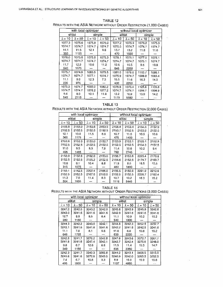
5.4 Results Obtained Without Order Restriction 5.4.1 The ASIA Network The results obtained with the different simulations of the ASIA network are shown in Tables 11,12,13,14. We observe that as the number of cases increases it becomes more difficult to find better results than the evaluation of the initial structure. For example, for the 500 cases database, we see that except for the algorithms without local optimizer, that use the simple selection criterion, all algorithms give, on average, better values than the initial structure evaluation. For the database of 1,000 cases, this observation can be done for all algorithms except for the ones that use simple reduction and a high mutation probability. With the 2,000 case database, on average, there are better results found than the initial structure evaluation by the elitist algorithms that incorporate the local optimizer, by the algorithms with the local optimizer that use simple reduction and a low mutation probability, and by the elitist algorithms that do not contain the local optimizer and have a large population size. The absence of the local optimizer in combination with simple reduction, low mutation probabilities and large population sizes also give, on average, better results than the evaluation of the initial structure. Finally, for the 3,000 case database, the best results were found using an elitist algorithm with a large population size, by algorithms that incorporate the local optimizer, that use simple reduction and a low mutation rate and by elitist

20,433 18,885 101.5 102.8

- -

22,016 20,986 20,931 20,687 100.0 102.0

- -

22,998 22,469 22,312 22,114 101.1 99.9

- -

23,259 22,508 22,201 21,827 103.0 103.3

- -

algorithms that contain the local optimizer and that have a high mutation probability.

With regard to the statistical significance of the analyzed parameters, for all databases we find that with respect to the evaluation function, statistically significant differences exist in the use of the local optimizer, the reduction criterion, the population size and the mutation probability. With respect to the Hamming distance statistically significant differences exist in the use of the optimizer and in the population size. Moreover, significant differences are detected with the 500 and the 1,000 case databases in the mutation probability, with the 2,000 case database in the selection criterion.

Concerning the AHD values, we observe that the effect of the parameters is similar to the one described in Section 5.3.1. The worst performance is found with no hybrid algorithms that use simple reduction and have a high mutation rate. For the rest of the algorithms the AHD takes a value of about 10, independent of the size of the database.

With respect to the ANE value, the algorithms with a population size of 50 evaluate about 4 times more structures than the algorithms with a population size of 10. In general the ANE value increases as the mutation rate grows.

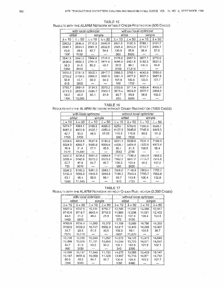
5.4.2 The ALARM Network The results obtained are represented in Tables 15,16,17,18. Like with the ASIA network, we observe that as the simulation size grows it becomes more difficult to find parameter combinations for the genetic algorithm that obtain structures with better evaluations than the initial structure.

For the 500 case database, we observe a good performance of the elitist hybrid algorithms as well of the simple hybrid algorithms that have a low mutation rate. Only two parameter combinations result in better average results than the evaluation corresponding to the ALARM network structure. There are 4 elitist hybrid algorithms with a low mutation rate and one simple hybrid algorithm (a = 50, pm = 0.01, and pc = 0.5) that have better evaluations than the initial structure.


For the 1,000 case database, only the elitist hybrid algorithms with population size 50 and a low mutation rate result in a better evaluation than that of the one of the initial network structure. Moreover, the elitist hybrid algorithm that has a population size 10 and a high crossover probability has found a better evaluation than the one of the ALARM network.

With 2,000 cases, the best results were obtained with the elitist hybrid algorithms with pm = 0.01, as well as with the simple hybrid algorithm with A = 50, pC = 0.5, and pm = 0.01. None of the parameter combinations give on average a better performance than the initial structure. For some parameter combinations, however, some results were found that were better than the ALARM network evaluation.

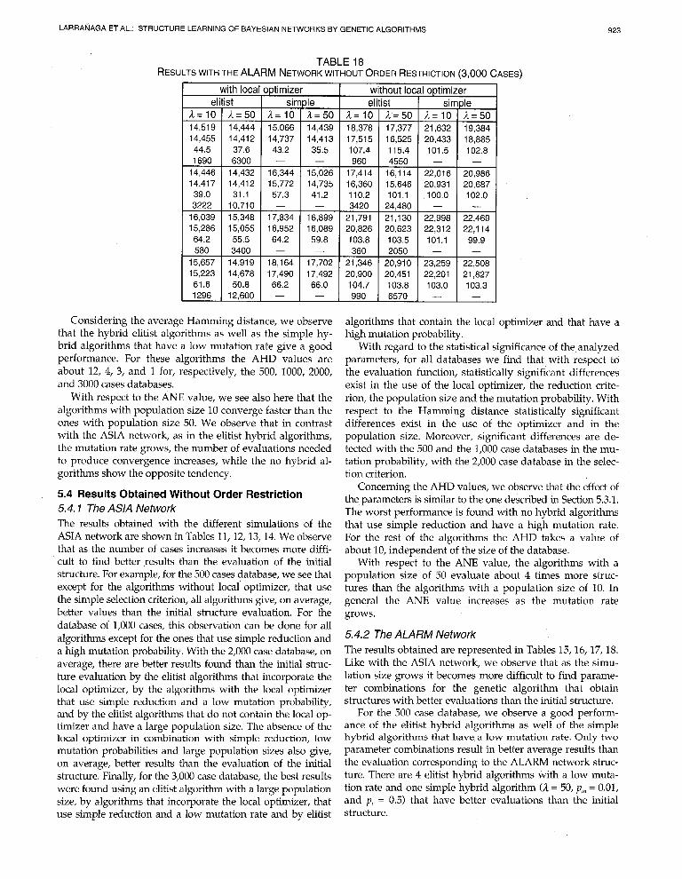
For the 3,000 case database, the best results were obtained with the elitist hybrid algorithms that had a low mutation rate, as well as with the simple hybrid algorithm with il = 50, p, = 0.01, and pC = 0.5. None of the searches found better results than the ALARM network evaluation, but in both of them we found the same evaluation than that of the initial structure.

With respect to the statistically significant differences in the evaluation function, for all four databases a similar behavior was detected. Significant differences are found with respect to the use of the local optimizer, the reduction criterion, the population size and the mutation rate. In the Hamming distance statistically significant differences are detected, for all the four databases, with respect to the use of the local optimizer and the mutation rate. For the 500 case database, significant differences in the Hamming dis- tances also exist with respect to the reduction criterion. The best values of the average Hamming distance are obtained with elitist hybrid algorithms that have a low mutation rate as well as by simple hybrid ones that have low mutation and crossover rates. In these algorithms the AHD takes a value between 35 and 40.

An algorithm with population size 10 evaluates about l/5 of the number of structtires that an algorithm with population size 50 evaluates.

6 CONCLUSIONS AND FURTHER RESEARCH We have presented a method for structure learning of Bay- esian networks from a database of cases. The method is based on genetic algorithms. To guarantee the closeness of the genetic operators, we have devised a repair operator.

Using simulations of the ASIA and ALARM networks, we carried out a performance analysis on the control parameters of the genetic algorithms (population size, local optimizer, reduction mechanism, probability of crossover, mutation rate). The obtained results indicate that in using genetic algorithms in the structure learning of BNs, it is recommended to use a hybrid algorithm that uses elitist reduction in combination with a not too small population size and a relatively low mutation rate. This is even more true if no ordering restriction between the nodes is assumed.

It would be interesting to experiment with a repair operator that does not break cycles by deleting arcs at random, but by some optimization criterion or with a repair operator based on the fusion of two structures like in 1481.

In the future we want to extend the described structure learning approach based on genetic algorithms by trying to find the optimal ordering of the system variables. We think to tackle the search for an optimal ordering with a genetic algorithm that uses genetic operators that were used in the tackling of the Traveling Salesman Problem.

We also plan to adapt the described structure learning approach to dynamic BNs [49]. In other two problems related to Bayesian networks of which we expect that they can be tackled successfully with genetic algorithms are the so-called optimal decomposition of a BN, and the fusion of mul- tiple authors BNs.

APPENDIX-BASIC DEFINITIONS DEFTNITION 1. a) An instance of an optimization problem is a

pair (D, f) where D is the domain of the feasible points, and f is the cost function. The problem is to find a w E D fey which f(w) I f(y) fey all y E D. 6) An optimization problem is a set I of instances of an optimization problem.

DEFINITION 2. An encoding of a domain D is a function e : D + S’, where S is the alphabet, S’ is the search space, and 1 2 1% IISII II D II

Thus the encoding of the elements of D is a mapping from the domain D to the strings of length 1 over S.

DEFINITION 3. g(x) = f(e(x)), the composition of the functions f and e, is the objective function.

Suppose that ;li denotes the size of the population of the genetic algorithm at time t. To simplify, we assume that 4 = ?L for every t. P, denotes the population at time t.

P, = {Ii, , It’], where I/( j = 1, , a.) denotes the jth individual of the population at time t, and 1: = (sl, , sl),

where s,(w = 1, . . . . 1) are elements of the alphabet S. PS, de; notes the set of populations of size il.

In the following, and without loss of generality, we will not use the t index.

DEFINITION 4. The global selection function, fsel, selects randomly with reemplacement a collection y E PS, from a population x E PSn:

fsel: (a, 4 -+y, where a is a vector of dimension ;1 of randomly chosen values.

DEFINITION 5. The selection function is based on the rank of the objective function if the probability that Ii becomes a parent is proportional to the rank of its evaluation. This means that:

pp,,entUi) = r(rank(gU’)))

where r is a decreasing function of the rank of g(l’), and rank (g(l’)) = d ti 3d - 1 individuals with better evaluation function than Ii.

As an example of this kind of selection function, we have:

r(yank(l’l) = il + 1 - rarzk(g(1’))

qa + q/2

LARRAtiAGA ET AL.: STRUCTURE LEARNING OF BAYESIAN NETWORKS BY GENETIC ALGORITHMS 925

DEFINITION 6. The global production function, fprod, produces offspring z E PS, from selected individuals y E PS, using a crossover operator:

where p is a vector of dimension A of randomly chosen in- teger values from 1 to il.

DEFINITION 7. The production finnctiqn is one point crossover if the parents Ii = (sl, . . . . SJ and I’ = (b,, . . . . b,) produce children CH”‘l = (c,, . . . . q) and CH”‘* = (d,, . . . . d,) verifiying:

1

si ifjrm ‘i= bj ifj>m

di = {

bj ifj<m sj ifj>m

where m is taken from the uniform distribution defined on the interval [l, I].

DEFINITION 8. The individual mutation function, fmdemut, applied to individual I = (sI, . . . . s,), generates another individual MI = (sm,, . . ., smd, that is findmmut (II = MI, such that Vj E (1, . ..I 11, P(smj = sj) = 1 - pm, where pm is the mutation probability.

DEFINITION 9. The extension function, fext, creates from two populations x, z E PS,, a population n E ES,,:

fez,: (x, 2) -3 n. Denoting by IV, with i = 1, . . . . 2il the ith individual in n, and by X,, with k = 1, . . . . ;1 the kth individual in x, and by Zj with j = 1, . . . . il the jth individual in z, we have:

Ni = i Xi ifi1;3. Zi-, ifi>A

DEFINITION 10. The global reduction function, fred, converts a population n E PS,, to a population r E PS,

ficd : n +r.

Notice that r denotes the population of individuals at time t + 1.

DEFINITION 11. The reduction function is elitist of degree A if the population at time t+l is formed by selecting the best A individuals-taking into account the objective function- among the A individuals of the population at time t and the offspring derived from them.

DEFINITION 12. The reduction,function is simple if the population at time t + 1 is formed by the offspring derived from the population at time t. Using the notation introduced in definitions 6, 9, and 10, the reduction function will be simple ifand only if r = z.

ACKNOWLEDGMENTS We wish to thank Gregory F. Cooper for providing his simulation of the ALARM Network. We also thank the refe- rees for their work and comments. This work was sup- ported by the Diputaci6n Foral de Gipuzkoa, under grant OF 95/1127, and by grant PI94/78 of the Gobierno Vasco.

REFERENCES Ill

[21

[31

[41

I51

161

I71

181

191

[lOI

1111

[121

1131

[I41

[I51

M

u71

1181

[I91

[201

1211

[221

P31

1241

J. Pearl, Probabilistic Reusoning in Intelligent Systems: Networks of Plausible Inference. San Mateo, Calif.: Morgan Kaufmann, 1988. R.E. Neapolitan, Probabilistic Reasoning in Expert Systems. Theory and Algorithms. John Wiley & Sons, 1990. F.V. Jensen, “Introduction to Bayesian Networks,” Technical Re- port IR 93-2003, Dept. of Mathematics and Computer Science, Univ. of Aalborg, Denmark, 1993. C.K. Chow and C.N. Liu, “Approximating Discrete Probability Distributions with Dependence Trees,” IEEE Trans. Informution Theory, vol. 14, pp. 462-467,1968. G. Rebane and J. Pearl, “The Recovery of Causal Polytrees from Statistical Data,” Uncertainty in Artificiul Intelligence, vol. 3, pp. 175- 182,1989. S. Acid, L.M. De Campos, A. Gonzalez, R. Molina, and N. Perez de la Blanca, “Learning with CASTLE,” Symbolic and Quantitative Approaches to Uncertainty, R. Kruse and P. Siegel, eds., Lecture Notes in Computer Science 548. Springer-Verlag, 1991. R.M. Fung and S.L. Crawford, “CONSTRUCTOR: A System for the Induction of Probabilistic Models,” Proc. AAAI, pp. 762-769,199O. E. Herskovits and G. Cooper, “Kutatb: An Entropy-Driven Sys- tem for Construction of Probabilistic Expert Systems from Data- bases,” Report KSL-90-22, Knowledge Systems Laboratory, Medi- cal Computer Science, Stanford Univ., 1990. G.F. Cooper and E.A. Herskovits, “A Bayesian Method for the Induction of Probabilistic Networks from Data,” Machine Leurn- ing, vol. 9, no. 4, pp. 309-347,1992. R.R. Bouckaert, “Probabilistic Network Construction Using the Minimum Description Length Principle,” Lectures Notes in Com- puter Science 747, Symbolic and Quantitative Approaches to Reasoning and Uncerfuinty, ECSQARU ‘93, pp. 41-48,1993. D. Wedelin, “Efficient Algorithms for Probabilistic Inference Combinatorial Optimization and the Discovery of Causal Struc- ture from Data,” doctoral dissertation, Chalmers Univ. of Tech- nology, GGteborg, 1993. S.L. Lauritzen, B. Thiesson, and D.T. Spiegelhalter, “Diagnostic Systems Created by Model Selection M>thGds-A Case &dy,” Proc. Fourth lnf’l Workshop Artificiul lntelliaence and Statistics, PP. 93- , , .A1 105,1993. CF. Aliferis and G.F. Cooper, “An Evaluation of an Algorithm for Inductive Learning of Bayesian Belief Networks Using Simulated Data Sets,” Uncertainty in Artificiul Intelligence, Proc. 10th Conf. , pp. 8-14,1994. R.R. Bouckaert, “Optimizing Causal Orderings for Generating DAGs from Data,” Uncertainty in Artificial Intelligence, Proc. Eighth Conj. , pp. 9-16,1992. R.R. Bouckaert, “Properties of Bayesian Belief Networks Learning Algorithms,” Proc. Uncertuinty in Artificial Intelligence, 10th Ann. Conf., pp. 102-109, Washington, D.C., 1994. D.hi. &ickering, D. Geiger, and D. Heckerman, “Learning Baye- Sian Networks: Search Methods and Experimental Results,” Fifth lnt’l Workshop Artificiul Intelligence and S&istics, pp. 112-128,19<5. D. Heckerman, D. Geiger, and D.M. Chickering, “Learning Baye- sian Networks: The Combination of Knowledge and Statistical data,” Technical Report MSR-TR-94-09, Microsoft, 1994. W. Lam and F. Bacchus, “Learning Bayesian Belief Networks. An Approach Based on the MDL Principle,” Compututionul Intelli- gence, vol. 10, no. 4,1994. W. Lam and F. Bacchus, “Using Causal Information and Local Measures to Learn Bayesian Networks,” Uncertainty in Artificial liztelligence, Proc. Ninth Conj., pp. 243-250,1993. D. Madigan, A.E. Raftery, J.C. York, J.M. Bradshaw, and R.G. Almond, “Strategies for Graphical Model Selection,” Proc. Fourth Int’l Workshop Artificial Intelligence and Statistics, pp. 331-336, 1993. R. Mechling and M. Valtorta, “PaCCIN: A Parallel Constructor of Markov Networks,” Proc. Fourth Int’l Workshop Artificial Intelli- gence and Statistics, pp. 405-410,1993. G.M. Provan and M. Singh, “Learning Bay&an Networks Using Feature Selection,” Preliminary Papers Fifth Int’l Workshop Artificiul Intelligence and Statistics, pp. 450-456, Florida, 1995. G.M. Provan, “Model Selection for Diagnosis and Treatment Us- ing Temporal Influence Diagrams,” Proc. Fourth Int’l Workshop Ar- tificial Intelligence and Statistics, pp. 469-480, 1995. M. Singh and M. Valtorta, “An Algorithm for the Construction of Bayesian Network Structures from Data,” Uncertainty in Artificial Intelligence, Proc. Ninth Conf., pp. 259-265, 1993.

926

L'51

1261

WI

m

1291

t301

[311

WI

[331

1341

[351

061

[371

[381

[391

[401

1411

Ml

[431

I441

[451

[461

[471 [481

[491

IEEE TRANSACTIONS ON PATTERN ANALYSIS AND MACHINE INTELLIGENCE, VOL. 18, NO. 9, SEPTEMBER 1996

I. Suzuki, “A Construction of Bay&an Networks from Databases Based on an MDL Principle,” Uncerfainfy in Artificial Intelligence, Proc. Ninth Conf., pp. 266-273,1993. P. Larrafiaga and Y. Yurramendi, “Structure Learning Ap- proaches in Causal Probabilistics Networks,” Symbolic and Quanfi- tative Approaches to Reasoning and Uncertainty, M. Clarke, R. Kruse, and S. Moral, eds., Lecture Notes in Computer Science 747, pp. 227. 232. Springer-Verlag, 1993. H.J. Bremermann, M. Rogson, and S. Salaff, “Search by Evolu- tion,” Biophysics and Cybernetic Systems, M. Maxfield, A. Callahan, and L.J. Fogel, eds. , pp. 157-167. Washington, D.C.: Spartan Books, 1965. I. Rechenberg, Optimierung technischer Systeme nach Prinzipien der biologischen Information. Stuttgart: Frommann Verlag, 1973 (in German). J.H. Holland, Adaptation in Natural nnd Artificial Systems. Ann Arbor, Mich.: Univ. of Michigan Press, 1975. D.E. Goldberg, Genetic Algorithms in Search, Optimization and Ma- chine Learning. Reading, Mass.: Addison-Wesley, 1989. Handbook of Genetic Algorithms, L. Davis, ed. New York: Van Nos- trand Reinhold, 1991. L.J. Fogel, “Autonomous Automata,” Ind. Res., vol. 4, pp. 14-19, 1962. H.-P. Schwefel, Numeriscke Optimierung van Computer-Modellen miffels der Evolutionsstrategie. Basel: Birkhauser, 1977 (in German). A.E. Eiben, E.H.L. Aarts, and KM. van Hee, “Global Convergence of Genetic Algorithms: An Infinite Markov Chain Analysis,” Computing Science Notes, Eindhoven Univ. of Technology, 1990. C. Janikov and 2. Michalewicz, “On the Convergence Problem in Genetic Algorithms,” UNCC technical report, 1990. R.F. Hartl, A Global Convergence Proof for II Class of Genefic Algo- rithms. Univ. of Technology, Vienna, 1990. U.K. Chakraborty and D.G. Dastidar, “Using Reliability Analysis to Estimate the Number of Generations to Convergence in Genetic Algorithms,” Information Processing Letters, vol. 46, no. 4, pp. 199- 209,1993. G. Rudolph, “Convergence Analysis of Canonical Genetic Algo- ritms,” IEEE Trans. Neural Networks, vol. 5, no. 1, pp. 96-101,1994. P. Larrafiaga and M. Poza, “Structure Learning of Bayesian Net- works by Genetics Algorithms,” Studies in Classification, Data Analysis, and Knowledge Organization, E. Diday, ed., pp. 300-306. Springer-Verlag, 1994. I’. Larrafiaga, R.H. Murga, M. Poza, and C.M.H. Kuijpers, “Structure Learning of Bayesian Networks by Hybrid Genetic Al- gorithms,” Preliminary Papers Fifth Int’l Workshop Artificial Infelli- gence and Statistics, pp. 310-316,1995. R.W. Robinson, “Counting Unlabeled Acyclic Digraphs,” Lecfures Notes in Mathematics 622: Combimzforial Mathematics V, C.H.C. Lit- tle, ed. , pp. 28-43. New York: Springer-Verlag, 1977. K.HGffgen, “Learning and Robust Learning of Product Distribuc- tions,” Technical Report 464, Fachbereich Informatik, Universitgt Dortmund, 1993. S.L. Lauritzen and D.J. Spiegelhalter, “Local Computations with Probabilities on Graphical Structures and Their Application on Expert Systems,” J. Royal Statistical Sot. B, vol. 50, no. 2, pp. 157. 224,1988. M. Henrion, “Propagating Uncertainty in Bayesian Networks by Probabilistic Logic Sampling,” Uncertainty in Artificial Intelligence, vol. 2, pp. 149-163,1988. I.A. Beinlinch, H.J. Suermondt, R.M. Chavez, and G.F. Cooper, “The ALARM Monitoring System: A Case Study with Two Prob- abilistic Inference Techniques for Belief Networks,” Proc. Second Europeax Conf. Artificial Iyltelligence in Medicine, pp. 247-256, 1989. E.H. Herskovits, “Computer Based Probabilistic-Network Con- struction,” doctoral dissertation, Medical Information Sciences, Stanford Univ., 1991. SPSS-X User’s Guide. third edition, 1988. 1. Matzkevich and B. Abramson, “The Topological Fusion of Bayes Nets,” Proc. Eighth Conf. Uncertainty in Artificial Intelligence, pp. 191-198,1992. U. Kjsrulff, “A Computational Scheme for Reasoning in Dynamic Probabilistic Networks,” Proc. Eighth Conf, Uncertainty in Artificial Infelligence, pp. 121-129,1992.

Pedro LarraAaga received the MSc degree in mathematics (mentions: statistics) from the University of Valladolid, Spain, in 1981, and the PhD degree in computer science from the Uni- versity of the Basque Country in 1995. Since 1985, he has been a lecturer in statistics and artificial intelligence in the Department of Com- puter Science and Artificial intelligence at the University of the Basque Country. His current research interests are in the fields of Bayesian networks, combinatorial optimization and data

analysis with applications to medicine, molecular biology, cryptoanaly- sis, and finance.

Mike1 Poza received the MSc degree in computer science from the University of the Basque Country in 1992. In 1993, he joined the Depart- ment of Computer Science and Artificial Intelli- gence of the University of the Basque Country, where he is currently working in data analysis.

Yosu Yurramendi received the MSc degree in mathematics (mentions: statistics and operations research) from Universidad Complutense of Ma- drid, Spain, in 1977, and the PhD degree in statistics (mention: data analysis) from Universitb Pierre et Marie Curie (Paris VI) in 1984. Since 1979, he has been a lecturer in statistics and artificial intelligence in the Computer Science and Artificial Intelligence Department at the University of the Basque Country. His research interests include data analysis and machine learning.

Roberto H. Murga received the MSc degree in computer science from the University of the Basque Country in 1994. In 1995, he collabo- rated with the Department of Computer Science and Artificial Intelligence of the University of the Basque Country. He is currently working at Telefonica, a firm in the telecommunications arena.

Cindy M.H. Kuijpers received the MSc degree in applied mathematics from the University of Technology of Eindhoven, the Netherlands, in 1993. She carried out her final project, which was within the field of combinatorial optimization, at the Philips Research Laboratories in Eindhoven, the Netherlands. Her Master’s thesis was awarded the VVS-prize 1994 of the Neth- erlands Society for Statistics and Operations Research (VVS). In 1994, she joined the De- partment of Computer Science and Artificial

Intelligence at the University of the Basque Country, where she is currently working on the use of genetic algorithms for tackling combinatorial optimization problems related to Bayesian networks.

912 IEEE TRANSACTIONS ON PATTERN ANALYSIS AND...

Documents

Transcript of 912 IEEE TRANSACTIONS ON PATTERN ANALYSIS AND...