9. Physical Layer Modeling - TU Berlin · 9. Physical Layer Modeling...

9. Physical Layer Modeling

A. de Baynast (European Microsoft Innovation Center)M. Bohge, D. Willkomm (Technische Universität Berlin)J. Gross (RWTH Aachen University)

The Physical Layer (PHY) is serving as the interface between the Data LinkLayer (DLL) and the environment. Accordingly, it defines the relation be-tween the device and the physical medium. In wireless systems, the generaltask of the PHY is to convert bit streams into radio waves and vice versa.Though the transmitter and the receiver are dual, they are comprised of dif-ferent components in the physical layer. The transmitter takes digital inputin form of (payload) bits and converts them into an analog signal, generallyaround a given carrier frequency which is then radiated via the antenna. Atthe receiver, this analog signal which has been distorted during the propa-gation is then converted back into a (payload) bit stream. The general goalof the PHY is to ensure that the bit stream at the transmitter and at thereceiver are identical. This is a very challenging task as the wireless channel(see Section 11) can distort and corrupt the analog signal in many different,random ways. In the following, we first provide an overview of the differentfunctionalities of the PHY at the transmitter and receiver as applied in mostcommon standards today like for cellular networks (such as Global Systemfor Mobile Communications (GSM), Universal Mobile TelecommunicationsSystem (UMTS), Long Term Evolution (LTE)) or local/metropolitan areanetworks (e.g. IEEE 802.11, IEEE 802.16) as well as for broadcast networks(Digital Audio Broadcasting (DAB), Digital Video Broadcasting (DVB)).Then we discuss common simulation approaches used in the PHY and theirshortcomings for network simulation. Finally, we comment on ways to includeselected aspects of the PHY in network simulation models.

9.1 Overview of the PHY Layer

In wireless systems the PHY layer can be subdivided into four domains asdepicted in Figure 9.1: the bit domain, the symbol domain, the sampledomain and the waveform/analog domain. Note that any layer above thePHY can be considered to be part of a fifth domain referred to as the "packetdomain", as indicated for the DLL in Figure 9.1. Data through the PHYlayer is sequentially represented in each of these domains, i.e., by packets,bits, symbols, samples and finally by waveforms.

136 9. Physical Layer Modeling

There are historical reasons behind this decomposition. Until the emer-gence of powerful processors in embedded communication devices during thelast two decades, the bit stream was directly transformed into waveforms,representing the information either by amplitude levels referred to as Am-plitude Modulation (AM) [375, Chap. 4, p.169], or by frequencies referredto as Frequency Modulation (FM) [395]. The corresponding waveform wasdirectly modulated by an oscillator set to a specific carrier frequency. At thereceiver, the analog signal was filtered by a matched filter in order to reducethe noise power outside the bandwidth of interest. In the particular case ofFM receiver [395], a simple Phase-Locked Loop (PLL) could be used to lockto the current frequency of the signal. Whereas the hardware implementationof such a receiver was extremely cheap, the spectral efficiency (i.e. the ratioof throughput over the required system bandwidth) remained low.As the demand for higher data rates increased dramatically over the last

two decades, designs of transmission systems with higher spectral efficiencyover broadband channels were required. Higher spectral efficiency has beenachieved by using more sophisticated transmission schemes, which in turn re-quire more complex algorithms especially at the receiver. In order to supportcomplex algorithms, the devices nowadays comprise of one or several digitalsignal processors[442] that support a significant number of the operationsrepresented in Figure 9.1. Besides the historical aspect, this decompositioninto different domains is also fundamental in the comprehension of the resultsand the limitations of any wireless network simulator since some of these do-mains correspond to the different abstraction levels used by simulation toolsas shown later. In this subsection, we first give a functional overview of thefour different domains of the PHY before we discuss single, functional ele-ments in the next subsection as second step.

Bit Domain. At the transmitter, a packet coming from the DLL enters thebit domain of the PHY. Three main functions are performed here: CyclicRedundancy Check (CRC) coding, Forward Error Correction (FEC) codingand interleaving. Firstly, CRC bits are added to the packet bits. The mainpurpose of CRC code is to detect at the receiver if an error occurred duringa transmission. Note that a CRC code only allows usually the detection oferrors, it does not allow the correction. In order to correct eventual transmis-sion errors, FEC coding schemes are used. Many different codes with differentcharacteristics are known today: for correcting only few errors (less than 1erroneous bit for 1000 bits transmitted) without penalizing the transmis-sion rate too much, Reed-Solomon (RS) codes are good candidates. If thetransmission channel introduces more errors (like typical GSM channels do),convolutional codes can be used. Even more efficient error correction codesare Turbo-codes [58] or Low-Density-Parity-Check (LDPC) codes [170, 300].While they are more efficient than convolutional codes, their decoding algo-rithms are more complex as they require several decoding iterations. However,most of the current communication standards support them at least as option

9.1 Overview of the PHY Layer 137

DATA LINK LAYER

Packet domain

DATA LINK LAYER

PHY LAYER

Bit domain

Resource

manager

Packet domain

CRC Checking

FEC EncodingCRC Insertion

Framing

CRC insertion

Framing

PHY LAYER

Bit domain

Symbol domain

Digital

modulation

Pilot/Preamble

insertion

Spreading OFDM (IFFT)

Symbol domain

Digital

demodulation

Pilot/Preamble

removal

Despreading OFDM (FFT)

FEC Decoding CRC

Frame sync

Channel

estimation/

equalization

Sample domain Sample domain

Pulse shaping

filterMatched filter

Energy

detection/

Carrier sensing

Energy

detection/

Carrier sensing

Synchronizatio

n

Analog domain

DAC

Analog domain

ADCIF up-

conversion

PLL

Antenna

beamforming

ACK

Space-time

coding

Space-time

decoding

IF down-

conversion

Interleaving De-interleaving

Segmentation

TRANSMITTER RECEIVER

ReassemblyACK insertion

...

UPPER LAYERS...

UPPER LAYERS

Network

Simulator

C,

Matlab

or

Labview

PLL

Fig. 9.1: Decomposition of the MAC and PHY layer into 5 domains for wirelesstransmission systems: the packet domain (MAC), the bit domain, thesymbol domain, the sample domain and the analog domain. A tentativelist (non exhaustive) of operations that enable reliable transmission be-tween the transmitter and the receiver in current transmission systems isalso represented in the figure. The operations are listed by domain whichcorresponds to the abstraction level in network simulators.


(like in UMTS, LTE, DVB or IEEE 802.11n). As the transmission errors oftenhappen in bursts [38], the coded bit stream is interleaved before transmissionso that the corresponding de-interleaver at the receiver will spread the biterrors uniformly within the received coded bit stream. All these operationsare realized on the bit stream (see the bit domain in Figure 9.1). However,this binary description of the transmit information is not sufficient for directmapping to an analog waveform in systems with higher spectral efficiency.

Symbol Domain. An intermediate step consists of transforming a bit or sev-eral bits into a symbol. Hence, the transmit information enters now the sym-bol domain. For instance, in an Amplitude Shift Keying (ASK) radio system,the symbol value represents the amplitude of the waveform. In FrequencyShift Keying (FSK) systems, the symbol value corresponds to a specific fre-quency taken from a pre-defined set. Hence, bits are still represented bydigital values but these are already “place-holders” for specific characteristicsof waveforms. In most today’s systems however, more advanced schemes areused. Typical bit-to-symbol mapping schemes are Gaussian Minimum ShiftKeying (GMSK) as used in GSM, Quadrature Amplitude Modulation (QAM)in IEEE 802.11, UMTS, LTE, IEEE 802.16, or Differential Quadrature PhaseShift Keying (DQPSK) in DAB/DVB. A description and a complete analy-sis of all these modulation schemes can be found in [375]. In order to sim-plify the design of the receiver, some pilot symbols and preamble or end-preamble are inserted. For instance, several null symbols are inserted beforeeach packet in IEEE 802.11 such that the beginning of a packet can be de-tected using a double sliding window algorithm. Recently, advanced transmis-sion schemes for broadband wireless communication have been proposed andsome of them have been deployed successfully. These advanced transmissionschemes are spread-spectrum, multi-carrier modulation and Multiple InputMultiple Output (MIMO) systems. In the particular case of spread-spectrum(which is used either for multiple access – see Section 10.1.4 – or for combatingfrequency selectivity of the transmission channels) each symbol is spread by aso-called spreading sequence of length equal to the spreading factor. In UMTSsystems, the spreading factor varies from 16 to 1024 such that multiple userscan simultaneously transmit in the same band without interfering with eachother since the spreading sequences are mutually orthogonal. Hence, the bit-to-symbol mapping leads to a few bits mapped to many modulation symbols(i.e. “spreading” the information over many symbols). This leads to a betterperformance in channels with inter-symbol interference. A further advancedtransmission scheme are multi-carrier modulation systems; the most success-ful example of such schemes is Orthogonal Frequency Division Multiplex(OFDM). An OFDM system combats efficiently the inter-symbol interferenceoccurring in frequency selective propagation channels [375, Chap.12, p.718]by applying the Digital Fourier Transform (DFT) at the receiver and its in-verse at the transmitter. This technique considerably simplifies the receiverimplementation in case of frequency-selective channels since it is much easier

9.1 Overview of the PHY Layer 139

to invert the channel effect in the frequency domain, i.e. after taking the DFToperation as long as it is done at the correct time lag (and assuming thatthe inverse of the coherence bandwidth of the channel does not exceed theguard interval of the system). Finally, a third advanced transmission schemeconsists of utilizing antenna arrays at the transmitter or at the receiver orat both sides. The main advantage of MIMO systems is to considerably in-crease the spectral efficiency of the system by exploiting the spatial diversity,as demonstrated in [158]. Three techniques for MIMO systems are generallyused. Firstly, beamforming consists of steering the energy of the signal to-wards the receiving antenna(s) by adjusting the weights of the phase arrayof the antennas [477]. The second technique is called space-time coding [457]which in contrary consists of spreading the energy spatially into all directionsin an uniform way such that all potential receivers can receive the signal. Fi-nally, the third technique consists of spatially multiplexing the emitted signalover all transmit antennas. Whereas considerable gains in terms of through-put and reliability are achieved, the drawback of these techniques is theircomputational complexity since matrix inversion of the channel coefficientsis often required at the receiver side.

Sample and Waveform Domain. The description of the transmit informationin terms of symbols is still not enough since it corresponds to a stream of con-secutive discrete values. However, there are several different ways to map thesymbols into waveforms, especially regarding the transition from one symbolto the next one. Most importantly, these different ways end up in differentbandwidths that the signal consumes in the frequency domain. The exacttransition from one symbol to the next one is governed by the so-called pulseshaping filters which limit the signal to the required bandwidth. Most of thecurrent systems are using a square-root raised cosine filter at the transmit-ter and receiver. This filter reduces the required bandwidth to a minimumwhile no symbol interference occurs (theory of the eye pattern [375, Chap.9]). As digital signal processors have become more and more powerful, thepulse shaping filtering is nowadays realized digitally. We refer to this level assample domain since the output of the filter are sampled at much higher ratethan the incoming symbols. The samples are then converted into an analogsignal by a Digital-to-Analog Converter (DAC) which is finally modulated tothe respective carrier frequency (for instance 2.4 GHz for 802.11, 1.6 GHz forLTE, 900 MHz or 1800 MHz for GSM, 400-700 MHz for DVB).It has to be mentioned that the whole process is performed by quite spe-

cialized hardware. In order to support a transmission rate of 10 or 20 megabitper second, the digital sequence representing the same information at thesample domain can easily consume a bit rate of several hundred megabit persecond. These information flows are processed by digital signal processingunits which realize all functions on dedicated hardware as ASIC or DSPs.This obviously also applies to the analog part (D/A conversion, mixing, am-plification) which is performed by a radio.


Compared to the transmitter, the receiver is far more complex in its func-tionality. This is mainly due to the processing steps of the sample domainsince the receiver needs to be synchronized in time and frequency (and possi-bly space for systems with multiple antennas) in order to accurately retrievethe symbols. In fact, a wireless receiver is usually able to detect and de-code transmit signals which are only a few decibel above the noise powerof the system (every electromagnetic system features some form of noisewhich interferes with very weak signals arriving from some transmitter –see Section 11.10). This requires quite sophisticated and specialized process-ing operations to be performed which relies on digital signal processors. Aftersynchronization the received signal basically works its way through the trans-mitter components in an opposite way.In the next section, we detail each operation at the transmitter and the

receiver into independent paragraphs with special emphasize on the compu-tational complexity. When the description of the operation at the receiveris dual of the operation at the transmitter, we describe the operation of thetransmitter and its counterpart function at the receiver within the same para-graph. We would like to insist that the list is not exhaustive. It provides anoverview of the main functions implemented in current wireless transmissionstandards. The purpose of the list is to give an overview of the operationscommonly utilized in current wireless transmission standards.

9.2 Description of the Main Components of the PHY

Layer

In this section, a brief description of the aforementioned components atthe transmitter and at the receiver is given. A complete list and explanationof all techniques used in the PHY layer is beyond the scope of this book.Furthermore, whereas the transmitter steps are clearly described in the stan-dards, the implementation of the receiver is left free for manufacturers andtherefore the exact operations at the receiver are generally not documentedin details. The following descriptions are intended only to give an overviewof the functional blocks present at a transmitter and receiver to the reader.For more details, the reader is asked to refer to the citations and referencestherein.

9.2.1 Components of the Bit Domain

Cyclic Redundancy Check Codes. CRC codes are hash functions designed todetect transmission errors. A CRC-enabled device calculates a short, fixed-length binary sequence, known as the CRC code, for each block of data(i.e. usually a frame, a header or a packet) and sends them both together.Generally, the CRC bits are padded at the end of the block. When a block is

9.2 Description of the Main Components of the PHY Layer 141

read or received, the device repeats the calculation. If the new CRC does notmatch the one calculated earlier, then the block contains a data error andthe device may take some action such as discarding the block (DAB, DVB,GSM, UMTS) or requesting the block to be sent again (WLAN). The termCRC code originates from the fact that the check code is redundant (it addszero information) and the algorithm is based on cyclic codes. CRC codes arepopular because they are simple to implement, and are particularly effectiveat detecting common errors caused by noise in transmission channels.All popular wireless systems are using CRC codes at the PHY (mostly

for header protection) and at the MAC layer (header protection as well aspayload protection). CRC codes are quite efficient at detecting the acciden-tal alteration of data. Typically, an n-bit CRC, applied to a data block ofarbitrary length, will detect any single error burst not longer than n bits andwill detect a fraction 1− 2−n of all longer error bursts. As errors in wirelesschannels tend to be distributed non-randomly, i.e. they are “bursty”, CRCcodes’ properties are more useful than any alternative schemes.

Forward Error Correction Codes. Encoding and decoding information viaFEC codes is a system of error control for data transmission, whereby thesender adds redundancy to the transmitted information using a predeter-mined algorithm, also known as an error-correction code. Each redundant bitis invariably a complex function of many original information bits. The orig-inal information may or may not appear in the encoded output; codes thatinclude the unmodified input in the output are called systematic, while thosethat do not are non-systematic. Contrary to CRC, FEC coding schemes allowthe receiver to correct errors (within some upper bound). The advantages ofFEC codes are that a feedback-channel is not required (as in GSM, UMTSsystems and broadcasting systems) or that retransmissions of data are dra-matically reduced in presence of a feedback-channel (as in IEEE 802.11 orLTE). This advantage comes at the cost of a lower throughput as redundancyis added to the bit stream. Given a FEC code of rate 1/3 generates 2 bits ofredundancy per information bit, which triples the bandwidth needed for thetransmission or equivalently reduces the effective throughput of the systemby a factor of three. The maximum fraction of errors that can be correctedis determined in advance by the design of the code, so different FEC codesare suitable for different transmission conditions.There are two main categories of FEC codes: Convolutional codes and

block codes [375, Chapter 8]. Convolutional codes work on bit or symbolstreams of arbitrary length. They are most often decoded with the Viterbialgorithm [166]. Viterbi decoding allows asymptotically optimal decoding ef-ficiency with increasing constraint length of the convolutional code, but atthe expense of exponentially increasing complexity with respect to the con-strained length. Most of the current wireless transmission standards (GSM,UMTS, LTE, IEEE 802.11, DAB, DVB) are using convolutional codes. Thecorresponding coding rate and constrained lengths are shown in Table 9.1.


GSM UMTS LTE IEEE 802.11 DVB-T

Coding rate 1/2 1/2-1/3 1/3-7/8 1/3-5/6 1/2-3/4Constrained length 7 7 (9) 7-9 7 8

Table 9.1: Coding rate of convolutional codes as used in the wireless transmissionstandards GSM, UMTS, LTE, IEEE 802.11, and DVB-T.

Block codes work on fixed-size blocks of bits or symbols of predeterminedsize. Practical block codes can generally be decoded fast due to their blocklength. There are many types of block codes, but among the classical onesthe most notable is Reed-Solomon (RS) coding. In current systems, blockcodes and convolutional codes are frequently combined in concatenated cod-ing schemes. A short constraint-length convolutional code with low codingrate does most of the work and a Reed-Solomon code with larger symbol sizeand block length corrects the few errors left by convolutional decoder. Dueto their order in the transmission chain, the Reed-Solomon and the convolu-tional codes are usually referred as outer and inner codes, respectively.Whereas the convolutional codes provide a good trade off between the

computational complexity and error-correction capability, there are otherFEC coding schemes whose performance is within few tenths of decibels ofthe maximal theoretical rate. The maximal theoretical rate is referred as theShannon limit in information theory [106]. The best known of these codesare the Turbo-codes [58] and the LDPC codes [170]. Although the complex-ity of the decoding is higher than for convolutional codes, their performanceis such that they are proposed in most of the current standards as optionalschemes (for example turbo-code of coding 1/3 in UMTS and LDPC in IEEE802.11n). The Turbo-codes and LDPC codes share the same decoding algo-rithm referred to as belief propagation, sum-product or sigma-pi [111, 268].This is an iterative algorithm for performing inference on graphical models,such as factor graphs that can be used to represent Turbo-codes and LDPCcodes. Several iterations are required before convergence as illustrated in Fig-ure 9.2.FEC codes have often an all-or-nothing tendency, i.e. they can perfectly

extract the transmitted message if the Signal-to-Noise-Ratio (SNR) of thetransmission channel is large enough and cannot correct any error if the SNRof the transmission channel is too small. Therefore, digital communicationsystems that use FEC coding tend to work well above a certain minimumSNR and not at all below. Typical values are 8 decibels in GSM and 10decibels for UMTS. This all-or-nothing tendency becomes more pronouncedthe more efficient the code works, i.e. the closer the FEC code approaches thetheoretical limit imposed by the Shannon capacity [106]. This is particularlytrue for the Turbo-codes, the LDPC codes and the concatenated schemeswith convolutional code as inner code and RS code as outer code.


0 1 2 3 4 5 610

−7

10−6

10−5

10−4

10−3

10−2

10−1

100

SNR (dB)

Bit error Rate

Uncoded BPSK

1 iteration

2 iterations

3 iterations

6 iterations

18 iterations

Fig. 9.2: Probability of bit error as a function of the signal-to-noise ratio of thetransmission channel and the number of iterations of the decoding algo-rithm. For Turbo-codes, 5 iterations are usually sufficient. The computa-tional complexity of the decoding algorithm is linear with respect to thenumber of iterations (data taken from [289]).

The performance gain of coded transmission compared to an uncodedtransmission is illustrated in Figure 9.3 and is referred as the coding gain.Finally, FEC coding schemes are often combined with puncturing (IEEE

802.11, LTE, DVB). Puncturing is a technique used to make the rate of a codeslightly higher than the basic rate of the code [194]. It is reached by deletionof some bits in the encoder output. Bits are deleted according to a puncturingmatrix. Punctured convolutional codes are also called “perforated”.

Bit Interleaving/De-Interleaving. Data is often transmitted with FEC codingthat enables the receiver to correct a certain number of errors which occurduring transmission. If a burst of bit-error occurs, the number of bit-errorswithin the same code word may exceed the threshold under which a correctionwould have been possible. In order to reduce the effect of such error bursts,the bits of a number of consecutive codewords are interleaved before beingtransmitted [390]. This way, the wrong bits of an error burst are spread overseveral code words, which makes the error correction of the overall bit streameasier to be accomplished.


0 2 4 6 8 10 12 1410

−10

10−9

10−8

10−7

10−6

10−5

10−4

10−3

10−2

10−1

SNR (dB)

Bit error Rate

(255,223,33) RS code

64−state conv. code

Uncoded BPSK

RS + conv. with infinite interleaving

RS + conv. without interleaving

Fig. 9.3: Probability of bit error as a function of the signal-to-noise ratio of thetransmission channel for several schemes: uncoded antipodal signal (un-coded BPSK), stand-alone convolutional code, stand-alone RS, concate-nated scheme (convolutional code + RS) with and without interleav-ing. For the same spectral efficiency, the performance of concatenatedschemes is superior to the performance of uncoded scheme or stand-alone FEC schemes especially for lower probability of bit error (datataken from [375]).


9.2.2 Components of the Symbol Domain

Digital Modulation/Demodulation. Digital modulation and demodulation isthe process of transforming a chunk of consecutive bits into one or severalparameters of a sine wave (at the transmitter) and back (at the receiver).Note that digital modulation does not generate the waveform yet but it pro-duces a stream of waveform parameters which are turned at a later stageto an analog waveform. Modulating information onto a waveform usually in-volves varying one sine waveform in relation to another sine waveform. Thethree key parameters of a sine wave that can therefore carry information areits amplitude, its phase and its frequency. Digital modulation is sometimesreferred to as constellation mapping. The most common digital modulationtechniques are listed in Table. 9.2.

GSM UMTS LTE (IEEE 802.16) IEEE 802.11

GMSK QPSK 4/16/64-QAM BPSK-4/16/64-QAM4 bits/symb 2 bits/symb 2-8 bits/symb 1-8 bits/symb

Table 9.2: Types of modulation techniques used in wireless transmission standardsGSM, UMTS, LTE, IEEE 802.16, and IEEE 802.11.

In GSM systems, the GMSK modulation technique is employed. GMSK isa continuous-phase frequency-shift keying modulation scheme. It is similar tostandard Minimum Shift Keying (MSK) modulation [375, Chapter 5], how-ever the digital data stream is first shaped with a Gaussian filter before beingapplied to a frequency modulator. This has the advantage of reducing side-band power, which in turn reduces out-of-band interference between signalcarriers in adjacent frequency channels. However, the Gaussian filter increasesthe modulation memory in the system and causes inter-symbol interference,making it more difficult to discriminate between different transmitted datavalues and requiring more complex channel equalization algorithms such asan adaptive equalizer at the receiver.In UMTS, LTE, IEEE 802.16 and IEEE 802.11 systems, QAM is utilized.

It conveys two digital bit streams by modulating the amplitudes of two carrierwaves, using the ASK modulation scheme. These two waves, usually sinusoids,are out of phase with each other by 90 degrees and are thus called quadraturecarriers or quadrature components – hence the name of the scheme. Themodulated waves are summed, and the resulting waveform is a combinationof both Phase Shift Keying (PSK) and ASK. In the digital QAM case, afinite number of at least two phases, and at least two amplitudes are used (4-QAM). However, Binary Phase Shift Keying (BPSK) and Quadrature PhaseShift Keying (QPSK) modulations can be viewed as special cases of QAMmodulation. QPSK is equivalent to 4-QAM and BPSK has two amplitudes


but a single phase. The operation which consists of mapping bit(s) to a symbolis illustrated in Figure 9.4 in the case of QAM modulation.

00

01

10

11

Constellation 4−QAM

0000

0001

0011

0010

0100

0101

0111

0110

1100

1101

1111

1110

1000

1001

1011

1010


00000 00001

0001100010

00100

00101

00111

00110

01100

01101

01111

01110

01000

01001

01011

01010

11000

11001

11011

11010

11100

11101

11111

11110

10100

10101

10111

10110

1000010001

10011 10010


000000

000001

000011

000010

000110

000111

000101

000100

001000

001001

001011

001010

001110

001111

001101

001100

011000

011001

011011

011010

011110

011111

011101

011100

010000

010001

010011

010010

010110

010111

010101

010100

110000

110001

110011

110010

110110

110111

110101

110100

111000

111001

111011

111010

111110

111111

111101

111100

101000

101001

101011

101010

101110

101111

101101

101100

100000

100001

100011

100010

100110

100111

100101

100100


Fig. 9.4: Constellation of QAM signaling. Several bits are gathered to form oneQAM symbol. The higher the modulation order the more efficient is thetransmission. However, the distance between symbols becomes smaller asthe number of symbols increase and is more subject to errors in presenceof the transmission noise. In practice, 256 is the maximum supportedorder in wireless transmissions.

Pilot/Preamble Insertion and Removal. All digital wireless communicationsystems use pilot symbols in order to simplify the design of the receiver.Pilots are used to transmit data known in advance by the receiver. It usesthem to perform synchronization and channel estimation. There are severaltypes of pilots: preamble within the packet, few tones for OFDM systems,preamble for packet detection and null symbols for energy detection. The


type of pilots used in current wireless transmission standards are listed inTable 9.3.

GSM UMTS LTE, IEEE 802.16Training seq Training seq (Q) Preamble + Pilot Tones

25% of the resources 50% 30%

IEEE 802.11 DAB DVB-TPreamble + Pilot tones Preamble Preamble + Pilot Tones30% of the resources 5% 10%

Table 9.3: Types of pilot techniques used in wireless transmission standards.

Spreading/De-spreading. Spreading is an advanced transmission scheme usedfor broadband wireless channels. It is in a sense the simplest FEC codingtechnique employed in the symbol domain. In spread-spectrum a signalis generated which has a much larger bandwidth than would be requiredfor conveying the pure stream of information. There are three basic tech-niques employed to spread the information signal: direct sequence, frequencyhopping, or a hybrid of these. Spread spectrum makes use of a sequentialnoise-like signal structure to spread the information signal over a much widerband of frequencies. In direct sequence spread-spectrum, for example, eachbit of the information stream is mapped to a sequence of bits (where typicalratios – the spreading factor – between input bit to output bits are 1/16 or1/32 in UMTS, 1/11 in IEEE 802.11b). This sequence of bits is well-known inadvance and is referred to as spreading code. Then, the resulting “spreaded”bit stream is fed to a modulator which generates now many more modulationsymbols than would be required for the information stream. At the receiverthe incoming signal is correlated with the spreading code to retrieve the orig-inal information signal referred to as de-spreading. Clearly, for de-spreadingto work correctly, the transmit and receive spreading sequences must be thesame and they must be synchronized. This requires the receiver to synchro-nize its sequence with the transmitter’s sequence by taking the maximum ofthe cross-correlation function between the spreading code and received data.Good spreading codes are designed to appear as random sequences, i.e. nothaving long trails of 1’s or 0’s and overall almost the same number of 1’s and0’s. Due to the pseudo-randomness of the spreading sequence, the resultingsignal resembles white noise. Spreading by frequency hopping works in a simi-lar manner. Here, a single bit is converted to one or several “hops” in frequencyaccording to a predetermined sequence. Spread-spectrum has several advan-tages. First of all, it decreases the potential interference to other receivers asthe transmit power of the spreaded signal is quite low. This does not harmthe reception of the signal as the receiver – which knows the spreading se-


quence – sums up the transmit energy over 16 symbols in case of a spreadingfactor of 1/16 and can therefore tolerate a transmit power which is lower by afactor of 16 (equaling 12 dB). Furthermore, spread-spectrum signals mitigateinter-symbol interference caused by frequency-selective fading channels as asingle bit is converted – in direct sequence spread spectrum with a factor of1/16 – into 16 channel bits which achieves quite a coding gain. This effecteven can be enhanced to resolve dominant paths of a multipath propagationenvironment known as RAKE receiver [446]. It is implemented in most of theUMTS receivers today. Furthermore, spread-spectrum enhances privacy asthe spreading code has to be known to successfully decode the signal. With-out knowing the spreading code, it is even hard to only detect the signal asthe required transmit power for a large spreading factor is quite low. Due tothese reasons, spread-spectrum systems were first developed by the militaryand are still widely applied there. Finally, spread-spectrum systems enablemultiple access by assigning different data transmissions different spreadingcodes (in case of direct sequence spread-spectrum the corresponding multipleaccess schemes is referred to as Code Division Multiple Access (CDMA), seeSection 10.1.4).In current wireless standards, the two main spread-spectrum techniques

are frequency hopping spread-spectrum (Bluetooth) and direct-sequencespread-spectrum (Global Positioning System (GPS), UMTS, IEEE 802.11b).In UMTS (and IS-95, CDMA2000) direct-sequence spread-spectrum is alsoapplied for multiple-access. Its principle is illustrated in Figure 9.5.

−12 MHz −8 MHz −4 MHz 0 MHz 4 MHz 8 MHz 12 MHz

0

0.2

0.4

0.6

0.8

1

X(f)

After spreading

No spreading

Fig. 9.5: Illustration of the spread spectrum technique. It consists of spreadingspectrally the transmitted signal such that the signal is less sensitive tothe frequency selectivity of the propagation channel or the interference ofthe other users in case of multiple-access scenario. As spreading sequencethe one of IEEE 802.11b is considered: 1,−1, 1, 1,−1, 1, 1, 1,−1,−1,−1.


Orthogonal Frequency Division Multiplexing. is an advanced Frequency Divi-sion Multiplex (FDM) transmission scheme for broadband wireless commu-nication channels. A large number of closely-spaced orthogonal subcarriersare used to carry data. The payload data is divided into several parallel datastreams or channels, one for each subcarrier. Each subcarrier is modulatedwith a conventional modulation scheme (such as QAM, see the descriptionabove on “Digital Modulation”) at a low symbol rate, maintaining total datarates similar to conventional single-carrier modulation schemes in the samebandwidth. This is achieved by taking the inverse DFT of the set of modula-tion symbols (one for each subcarrier) and processing afterwards the streamof samples representing the time domain signal. At the receiver, the timedomain samples are then transformed back by a DFT to the frequency do-main to retrieve the modulation symbols per subcarrier. OFDM has devel-oped into a popular scheme in modems for wired transmission over phonelines applied in Digital Subscriber Line (DSL) systems as discrete multi-tonemodulation, providing quite large rates for data communications. However,today it is also applied in wireless digital systems such as DVB, DAB andwireless local/cellular systems (IEEE 802.11a/g/n, LTE, IEEE 802.16). Theprimary advantage of OFDM over single-carrier schemes is its ability to copewith severe channel conditions - for example, narrow-band interference orfrequency-selective fading due to multipath - without complex equalizationfilters. Channel equalization is simplified because OFDM may be viewed asusing many slowly-modulated narrow-band signals rather than one rapidly-modulated wide-band signal. The low symbol rate makes the use of a guardinterval between symbols affordable, making it possible to eliminate Inter-symbol Interference (ISI). Although OFDM has been successfully deployed,it has still some disadvantages compared to single carrier systems: sensitiv-ity to Doppler shift, sensitivity to frequency synchronization problems whichrequires generally a complex synchronization unit at the receiver as well asa high peak-to-average-power ratio, i.e. large power difference between theweakest and the strongest amplitudes on subcarriers. Finally, the loss of spec-tral efficiency caused by cyclic prefix/guard interval might not be negligible.For instance, the loss is about 20% in IEEE 802.11 a/g/n systems.OFDM in its primary form is considered as a digital modulation technique

since it is utilized for conveying one bit stream over one communication chan-nel using one sequence of OFDM symbols. However, OFDM can be combinedwith multiple access using time, frequency or coding separation of the users.One particular important multiple access combination with OFDM is thefrequency separation referred to as OFDMA, see Section 10.1.2. It is appliedtoday in LTE and IEEE 802.16e systems.

The next two paragraphs discuss three techniques for transmission sys-tems with multiple inputs or/and multiple outputs (in general summarized


under the acronym MIMO). Interest for MIMO systems has considerably in-creased over the last decade for two main reasons: the throughput increaseslinearly with the number of inputs and the probability of transmission errorsdecreases linearly with the number of receive antennas for basic scheme. Thesecond reason is that current powerful processors can support such techniquesin wireless standards (UMTS, LTE, IEEE 802.16).

Antenna Beamforming. Beamforming is a signal processing technique usedin wireless transmission systems for directional signal transmission or recep-tion. It exploits “spatial selectivity” among a single signal transmitted frommultiple antennas, or received by multiple antennas, or both. If beamform-ing is applied at the transmitter, the same transmit signal is sent from eachantenna. However, a beamformer controls the phase and relative amplitudeof the signal at each antenna in order to create a pattern of constructive anddestructive interference in the wavefront. Effectively, this gives the signal apreferred direction such that the SNR at the receiver is strongly increased.However, the transmitter must know the position of the receiver (or evenbetter, its channel characteristics with respect to each transmit antenna).When applied for receiving, the incoming signal from different antennas iscombined in such a way by delaying some signals and multiplying with ade-quate complex coefficients (phase and amplitude). As a result, the receivedsignal’s SNR is strongly increased (but again the receiver has to know thedirection from which the transmitted signal is received or even better theexact channel characteristic). If both transmitter and receiver have multi-ple antennas, beamforming may also be applied both at the transmitter andthe receiver which leads to an even better SNR. However, beamforming canbe computationally expensive if applied for several antennas at the trans-mitter or receiver (while also requiring control overhead). Hence, only basicbeamforming techniques are being used in wireless standards today: Trans-mit antenna selection in GSM and UMTS which consists of selecting thetransmit antenna that provides the best SNR for the considered terminal.For LTE, a pre-coding based beamforming with partial Space Division Mul-tiple Access (SDMA) can be used optionally if the system supports MIMOtechniques. A flexible system is IEEE 802.11n, which permits the applicationof beamforming simultaneously at the transmitter and receiver, based on thechannel state information sent from the receiver to the transmitter by controlframes. This technique is sometimes referred to as closed loop beamforming.

Space-time Coding/Decoding. Also in case of wireless systems with multipletransmit antenna, Space Time Coding (STC) is another method employedto improve the reliability of data transmission. Space-time coding relies ontransmitting multiple, redundant copies of a data stream to the receiver inthe hope that at least some of them may “survive” the physical path betweentransmission and reception in a good enough state to allow reliable decoding.Space time codes may be split into two categories:


1. Space-time trellis codes [458] distribute a trellis code over multiple anten-nas and multiple time-slots and provide both coding gain and diversitygain.

2. Space-time block codes [427],[456] act on a block of data at once (similarlyto block codes) and provide only diversity gain, but are much less complexin implementation terms than space-time trellis codes.

UMTS, LTE and IEEE 802.11n support the basic Alamouti scheme [427].Alamouti invented the simplest of all the STBCs in 1998 [427]. It was designedfor a two-transmit antenna system and one receive antenna. It takes twotime-slots to transmit two symbols such that it can achieve its full diversitygain without needing to sacrifice its data rate. The significance of Alamouti’sproposal in 1998 is that it was the first demonstration of a method of encodingwhich enables full diversity with linear processing at the receiver. Earlierproposals for transmit diversity required processing schemes which scaledexponentially with the number of transmit antennas [157]. Furthermore, itwas the first open-loop transmit diversity technique which had this capability.Subsequent generalizations of Alamouti’s concept have led to a tremendousimpact on the wireless communications industry.

Spatial Multiplexing. If a transmitter has data to be sent to multiple re-ceivers and if it has multiple transmit antennas, it can actually transmitthe information to all terminals simultaneously. This is referred to as spatialmultiplexing [468]. In spatial multiplexing the transmit signal of the datafor each receiver is concentrated by beamforming on the location of the re-ceiver. However, this concentration in some preferred direction leads to astrongly attenuated signal transmitted into several other directions. Thesedirections are the ones where further receivers can be served without havingthem suffer from interference of a simultaneous packet transmission. Hence,not all receiver distributions can be supported in a similar manner by spatialmultiplexing. Spatial multiplexing is furthermore limited by the number ofantennas the transmitter has, i.e. for n antennas up to n terminals can beserved at the same point in time. In a similar manner a receiver with n an-tennas can receive up to n packets simultaneously by applying a beamformer.This is referred to as space division multiple access (see Section 10.1.3). Aswith spatial multiplexing, this works well for some transmitter position com-binations while other combinations can not be resolved by the beamformerefficiently. Furthermore, if the receiver has multiple antennas then the con-straint on the positions of the transmitters becomes less significant by theapplication of interference cancellation algorithms. In fact, the application ofinterference cancellation allows even for several, different packets transmit-ted over different antennas to the same receiver (if the receiver has multipleantennas as well). This is the most promiment MIMO scheme which is oftencharacterized by a linear increase of the system capacity with the (minimal)number of antennas at the transmitter and receiver side. However, the com-plexity of especially the receiver is currently a strong limitation factor. Still, it


is expected that this MIMO technique will be strongly used in future wirelessstandards.

Symbol Interleaving/De-Interleaving. Symbol interleaving is used in digitaldata transmission technology to protect the data against burst errors occur-ring during the propagation. As with bit interleaving, if a burst error occurs,too many errors can be made within one code word, and that code wordcannot be correctly decoded. To reduce the effect of such burst errors, thesymbols of a number of frames are interleaved before being transmitted. Thisway, a burst error affects only a correctable number of symbols in each frame,and the decoder can decode the frame correctly. LTE and DVB systems areusing symbol interleaving.

9.2.3 Components of the Sample and Waveform Domain

Frame/Packet Synchronization. Once a digital train of samples is obtained,the receiving circuits (in the digital domain) first have to synchronize tothe transmitter. This refers to fine tuning to the exact timing with whichthe modulation symbols are transmitted and to the exact carrier frequencyused by the transmitter (there is always some frequency shift between anytwo oscillators, hence, requiring the receiver to identify the shift and correctit). Special training sequences (also referred to as preambles) are added bythe transmitter to any data transmission which the receiver can use to easilyacquire a precise enough synchronization. However, if the transmission occursover a quite bad communication channel, already the step of synchronizationcan become very difficult and requires special design [406].

Channel Estimation and Equalization. After obtaining synchronization, thereceiver has to identify the possible random distortions that the wirelesschannel causes to the signal (like phase shifts and attenuations/gains). Thisis known as channel estimation. For this, so called pilot signals are added tothe transmit signal which are transmitted with a known strength and witha known phase. After the channel has been estimated, the distortions of thechannel are compensated which is known as equalization. The proper estima-tion and equalization of the channel is a prerequisite for decoding the payloadsignal (as synchronization is a prerequisite as well). As an alternate solution,differential modulation (DAB) can be utilized. Since the data information iscontained in the phase difference between two consecutive symbols, the datacan be retrieved if the phase shift occurring during the transmission is equalfor both symbols.

Pulse Shaping Filter/Matched Filter. In digital telecommunication, pulseshaping is the process of changing the waveform of transmitted pulses. Itspurpose is to make the transmitted signal suit better to the communicationchannel by limiting the effective bandwidth of the transmission. By filtering


the transmitted pulses this way, ISI caused by the channel can be reduced.Also, pulse shaping is essential for making the signal fit in its frequency band.Typically, pulse shaping is nowadays implemented in the digital domain be-fore the digital-to-analog conversion. Two main pulse-shaping filters are usedtoday in wireless communication systems: Either a Gaussian filter (like inGSM) or a raised-cosine filter [375, Chapter 9] (UMTS, LTE, IEEE 802.16,IEEE 802.11, DAB, DVB). The impulse response and the spectrum of theraised-cosine filter are plotted in Figure 9.6 for several values of roll-off factor� ranging from 0 to 1. The bandwidth occupied by the signal beyond the sam-pling frequency 1/2T is called the excess bandwidth and is usually expressedas a percentage of the sampling frequency. For example, when � = 0.22 asin UMTS standard, the excess bandwidth is 22%. The overall raised cosinespectral characteristic is usually split evenly between the transmitting pulseshaping filter and the receiving filter.

−3T −2T −T 0 T 2T 3T

−0.2

0

0.2

0.4

0.6

0.8

1

x(t)

−1/T −1/2T 0 1/2T 1/T

−0.2

0

0.2

0.4

0.6

0.8

1

X(f)

β=0.25

β=1

β=0.5

β=0

β=0

β=1β=0.25

β=0.5

Fig. 9.6: Impulse response (left) and spectrum (right) of the raised cosine filter forseveral values of roll-off factor �. Most of the current standards are usingraised cosine filter as pulse evenly split between the transmitter and thereceiver (GSM: 0.2, UMTS: 0.22, DAB: 0.3).

Carrier Sensing/Energy Detection. Carrier sensing is usually employed byCarrier Sense Multiple Access (CSMA) protocols, as employed for examplein the MAC of IEEE 802.11 systems. Through carrier sensing the transmitterevaluates the current state of the channel to determine whether the channel isidle or if it is currently busy with other data transmissions. There are differentpossibilities how to implement a carrier sensing algorithm. On the one handthere is energy detection which is purely checking for the current channelReceived Signal Strength Indication (RSSI). If the RSSI is above a certainthreshold – the so called Clear Channel Assessment (CCA) threshold – thechannel is declared busy. Alternatively, a wireless device might try to sensea decodable signal on the channel, for example a header of a certain wirelesssystem. Only if this header is decoded correctly, the channel is declared busy.The difference between this feature detection and pure energy detection isthat in the first case all devices operating in the corresponding bandwidth


can block the channel (by emitting energy) while in the second case onlyspecific devices can block the channel. Carrier sensing is also used duringthe association process in all cellular networks (GSM, UMTS, LTE) thatcomprise multiple channels operating on orthogonal carrier frequencies. Inthese cases, the SINR of each channel is evaluated by sensing a beacon oneach carrier.

DA/AD Conversion and IF Up/Down Conversion. In digital communica-tion digital-to-analog conversion is used to convert the pulse shaping filteredoutput into an analog voltage which will be sent to the radio front-end ofthe transmitter. At the receiver, the reverse operation is known as analog-to-digital conversion. By the Nyquist-Shannon sampling theorem, a sampledsignal can be reconstructed perfectly provided that the sampling frequencyis at least twice as big as the Nyquist frequency of the transmitted signalin absence of noise [106]. However, even with an ideal reconstruction filter,digital sampling introduces quantization errors that make perfect reconstruc-tion practically impossible. Increasing the digital resolution (i.e. increasingthe number of bits used in each sample) or introducing sampling dither canreduce this error.The performance of current digital-to-analog converters can support data

rates as high as 1 Gigasample per second [217] with 16 bit integer resolution.Therefore, the up-conversion of the baseband signal to an intermediate fre-quency with values ranging from 1 MHz to 10 MHz in most of the devicescan be done digitally.

9.3 Accurate Simulation of Physical Layers

With wireless transmission systems becoming more and more complexwhile the time-to-market is always decreasing, accurate simulations of up-coming standards are essential. Wireless communication standards becomeso involved due to the complexity of the system that the design and elabora-tion of the upcoming standards are done by means of using a simulator (andlater in the process a hardware prototype).Since most of the elementary operations in the components of the PHY

layer are done on vectors of bits or symbols or samples, natural candidatesare scientific programming languages, such as Matlab. As a point-to-pointcommunication can be modeled as a chain of elementary matrix or vectoroperations, it is also natural to consider in addition block diagrams as inMatlab Simulink or Labview. The simulations consist usually of evaluat-ing the symbol-, bit-, or packet-error rate of the transmitted PHY framesthat have been corrupted by the modeled transmission channel. In order totake the randomness of the transmission system into account (randomnessof the propagation medium, randomness of the transmitted data), a simula-tion provides the average performance for thousands of packet transmissions

9.3 Accurate Simulation of Physical Layers 155

with different transmission channel coefficients and different data to transmit.The simulation flow graph is illustrated in Figure 9.7. Most of these Matlab

PHY frame

generation of

pseudo-random

bits

Encoding,

modulation,

mapping

Generation of the

equivalent

transmission

channel (noise,

multipath, filtering)

Generation of the received PHY frame

Equalization,

demapping,

demodulation,

decoding

Bit/Packet error

rate updated

Fig. 9.7: Typical flow graph used for simulating performance of PHY layer trans-mission (Matlab, Labview, or C). The new algorithm(s) is (are) imple-mented either in the transmitter side (encoding, modulation) or on thereceiver side (equalization which includes interference canceler, decod-ing,. . . ).

implementations consider equivalent symbol timing and bypass network as-pects beside interference within PHY frames. Queuing, network topology,network protocols (TCP, IPv6) are rarely considered for complexity issuessince the computational complexity is increasing at least linearly each timea new random parameter is introduced (depth of the queue, location of thetransmitter/receiver). Moreover, the computational complexity of the sim-ulations increases polynomially (or even exponentially) with respect to thenumber of users so that the computational complexity of a simulation for afull cell is prohibitive and requires a higher level of abstraction as in the net-work simulators. However, this is basically not the main focus of Matlab or


Domains Bit rate (Mbits/s)

Bit domain 22.8 Mbits/sSymbol domain 28.5 Mbits/sSample domain > 914 Mbits/s

Table 9.4: Bit rate in the bit, symbol, and sample domains of the PHY layer forIEEE 802.11 system assuming a raw data rate of 10 Mbits/s at theMAC layer.

similar tools and there is no built-in libraries that allow networking consid-erations. Whereas their proposed environment allows fast development anddesign of advanced wireless techniques at the PHY layer, the next paragraphsdiscuss their main limitations. In the following we focus on three of them:

1. Slow execution speed:Whereas the Matlab environment is very conve-nient for developers, the fact that it is an interpreted language – especiallywhen loops cannot be avoided – makes the simulations extremely slow.To have a better understanding of the computational complexity, the bitrate in the different domains of the PHY layer is calculated in Tab. 9.4for IEEE 802.11 system with data rate of 10 megabits per second. Fromthis example, it is clear that scientific programming languages as Mat-lab can deal well with the bit and symbol domains, but not with thesample domains (the computational complexity is 2 orders of magnitudemore). One way to bypass this problem is to determine an equivalenttransmission model in the symbol domain. This is very commonly done.However, there is a risk that the equivalent model does not capture ac-curately some effect as sample synchronization or collision at the samplelevel. It is also possible to use C for accelerating some functions that arenot vectorial and require large sequential loops as in the Viterbi decoder.Matlab allows easily the integration of C functions (known as mex files).

2. No discrete-event support:While the sample or symbol processing ata transmitter or receiver imply a pseudo-continuous model of time, theprocessing steps of the higher layers of a wireless network happen muchmore asynchronous. In order to simulate this, discrete-event support isrequired, which is usually not provided. Furthermore, there is no librarysupport for functions of the higher layers, meaning that all functionalityneeds to be implemented from scratch.

3. Lack of interaction with network simulators: While Matlab canbe used via an interface for example from C code, the interfacing is notparticularly easy to handle nor is it quite fast.

9.4 Physical Layer Modeling for Network Simulations 157

9.4 Physical Layer Modeling for Network Simulations

From the previous sections it is clear that physical layer simulations arequite demanding with respect to computational complexity and the requiredbackground knowledge. Hence, the question arises how physical layer behaviorcan and should be modeled in the context of network simulation, i.e. thetypical simulation approach which only considers the packet domain.A brute force method interfaces between a network simulator and simu-

lator for the physical layer (like Matlab). While this provides a very detailedmodel, for larger deployments the approach does not scale with respect tocomplexity. Run times of simulations become so long, even for moderatelycomplex topologies, that there is no benefit left from the detailed simulationmodel. Furthermore, analyzing simulation results becomes much more diffi-cult as many more parameters have now an influence on the performance.Finally, as there is also a wide background knowledge required to design, ex-ecute and analyze such simulations, implementing the considered approachon a wireless prototyping platform might be a better choice. However, thereis still tool support for fully detailed simulation models of wireless systems. Aparticular tool that can combine the different “simulation worlds” of higherlayers (i.e. the simulators of the packet domain) and of the physical layer(among many other simulation domains) is Ptolemy from UC Berkeley [8].Still, the above mentioned complexity problems remain.Due to these reasons the common approach in wireless network simula-

tion is to abstract from the many details of the physical layer. More precisely,almost all physical layer models in network simulators aim at capturing thephysical layer impact on the transmission of frames or packets in terms ofthroughput, error probability and delay under the assumption of perfect syn-chronization. These models belong to the packet domain from Figure 9.1 andonly take the following functions into account: FEC coding, digital modula-tion, advanced transmission schemes (like OFDM, spread-spectrum, antennabeamforming and space-time coding) and carrier sensing. All the other func-tions are assumed to work perfectly without any performance degradation(which is a very strong assumption compared to reality). Thus, only thepacket error process (along with throughput and delay) can be taken intoaccount. These models can not provide a “bit-true” characterization of thePHY, where the impact of the PHY layer on the transmission of each bitis modeled accurately. The difference between these two approaches leadsto the important consequence that for packet-domain models only a state-ment can be derived if a packet/frame is received incorrectly but not whichbits are wrong (which can be obtained from a bit-true model). Knowing theposition of a bit error has some relevance for higher layers. If a header iscorrupted the packet is most likely discarded. On the other hand, if payloadbits are corrupted this may have quite different consequences for multime-dia applications like video or voice, which can tolerate some bit errors. Thequality degradation depends on the exact position of the bit error. However,


bit-true physical layer simulation models are much more complex regardingtheir implementation.Apart from other issues, two components are essential for all packet-

domain models. On the one hand, most packet-domain models determinethe channel quality between a transmitter and the corresponding receiver.Aspects of this step relate to considering path loss, shadowing, fading, noiseand interference in combination with the used antenna and possibly advancedtransmission schemes (like OFDM, spreading or MIMO systems). Another as-pect of this step involves the question if the channel quality is accounted foron the average or if an instantaneous channel quality is considered, i.e. onevalue or even multiple values per transmitted packet. On the other hand,most packet-domain models translate the channel quality into an error rate(mostly a bit-error rate). This mapping can be quite complex and involvesthe modeling of the digital modulation as well as the FEC scheme. In thefollowing, we give an overview of both modeling steps. Note that there arefurther aspects to be considered for a PHY layer packet-domain model, asdiscussed in Section 9.5.

9.4.1 Link-to-System Interface

In the following, we first discuss the mapping of the channel state to abit-error probability for narrow-band, single-carrier transmission systems, i.e.for systems without advanced transmission schemes assuming that the chan-nel gain is flat (see Section 11.7). For this we make in this section initiallythe assumption that the channel quality is fixed. This type of model is alsoreferred to as static channel (see Section 11.12). In this case we can find amapping of the channel state and the chosen transmission parameters (mod-ulation type, transmit power, coding scheme, etc.) into a resulting physicallayer behavior on the packet domain in terms of packet throughput, delayand bit-error rate. This mapping is referred to as link-to-system interface. Inits simplest form, it is based on the fact that for a certain received channelquality, as measured by the SNR, the bit error rate can be derived dependingon the chosen modulation type and transmit power. Once the bit error rate isdetermined, the corresponding packet error rate can be obtained as explainedin Section 10.2. The SNR is given by

=Ptx ⋅ ℎ

2

�2(9.1)

where Ptx is the transmit power, ℎ2 is the channel gain (see Chapter 11)

and �2 is the equivalent background noise power of the transmission. Thetransmit power Ptx is usually well known during network simulation, even ifit is adapted by the transmit node. Therefore, it is readily available for thecomputation of the SNR. This is also true for the noise power which depends


on specific PHY parameters of the receiver (see Section 11.10). Furthermore,ℎ2 denotes the channel gain between the transmitter and the receiver, whichwe assume to be constant initially. In this case the computation of the re-sulting bit error rate from a given SNR is rather easy and is also quite closeto the real system behavior. Either exact or approximate formulas are used,as derived in [100] for QAM systems. If no formulas exist, the consideredmodulation system might still have been investigated by related work pro-viding a SNR-to-BER curve. This curve can then be converted into a look-uptable to be used in the simulation. Finally, if no data on the modulationsystem exists, the only way to obtain an SNR-to-BER curve is to performextensive and accurate PHY simulations, for example using Matlab. Then,the obtained curve can be be mapped into a look-up table as shown in Ta-ble 9.5 for the four different modulation types of the IEEE 802.11b standardas taken from [355]. Given the bit-error rate, the next step is to determine the

SNR BPSK QPSK CCK5.5 CCK11(dB) (1Mbps) (2Mbps) (5.5Mbps) (11Mbps)

... ... ... ... ...-5 6e-2 0.5e0 0.5e0 0.5e0-4 2e-2 0.5e0 0.5e0 0.5e0-3 8e-3 0.5e0 0.5e0 0.5e0-2 4e-3 1e-1 0.5e0 0.5e0-1 1e-4 8e-2 0.5e0 0.5e00 3e-5 2e-2 0.5e0 0.5e01 1e-5 5e-3 8e-2 0.5e02 1e-6 1.2e-3 4e-2 0.5e0... ... ... ... ...

Table 9.5: An example Bit-Error Rate (BER) lookup table for the four different(uncoded) modulation types of the IEEE 802.11b Wireless Local AreaNetwork (WLAN) standard.

packet error rate. This step is described in detail in Section 10.2. Once thepacket error probability is obtained, for each transmitted packet a randomdecision is performed according to the packet error rate threshold and thecorresponding packet is then marked to be either erroneous or not.So far we have considered a static channel quality with a single modu-

lation type and a simple (single-carrier) transmission system. The mappingfrom SNR to bit-error rate gets already more complicated if a FEC codingscheme is assumed. To account for FEC coding, two general approaches exist.Either the coding effect is taken into account by modifying the SNR. In thiscase, coding simply “increases” the SNR leading to a better bit error rate.However, this assumes a constant coding gain between the coded and un-coded system which is usually not the case at high or low SNRs. Hence, onehas to obtain a detailed look-up table for the coded bit error rate of the FEC


codes in combination with the modulation scheme depending on the SNR.If such tables are not provided by books and research papers, they have tobe obtained from extensive physical layer simulations (usually performed inthe symbol- or sample domain of Figure 9.1). There are also limited ways tocapture the coded system behavior by formulas, see Section 12.1.2 for an ex-ample mapping for convolutional coding. Still, ultimately a packet error rateis obtained and for each transmitted packet a binary decision is performed ifthe packet is erroneous or not.Next, let us consider a varying channel gain. In wireless systems a vary-

ing channel gain is almost always encountered in reality. Hence, it is likely tobe included in a simulation study. The channel gain depends in general onthe distance between transmitter and receiver (therefore, the chosen mobil-ity model – see Section 14 – has an impact on the channel gain), but thereare also additional time-varying, random components to the channel gain re-ferred to as shadowing (see Section 11.6) and fading (see Section 11.7). Allthese effects ultimately lead to a varying ℎ2 in Equation 9.1 and thus theSNR varies over time. A quite common assumption for such cases is thatthe channel gain ℎ2 is constant during a single packet transmission but variesin between. Such channel models are also referred to as block-fading channels(see Section 11.12). This leads to determining an instantaneous SNR at thetime a packet is transmitted. From this instantaneous SNR an instantaneousbit-error rate is determined using the same method as above (formulas orlook-up tables for the modulation and coding scheme considered). Finally,a packet-error rate is determined and a random decision is performed if thepacket is received correctly or not. Depending on the considered distributionof the channel gain, this method can lead to a very different average packeterror rate behavior than considering a static channel quality. This is impor-tant to note if one is only interested in the average PHY layer behavior butfading or shadowing is to be taken into account.

9.4.2 Equivalent Channel Quality Models

The modeling of the channel quality and the corresponding PHY layerperformance becomes more complicated if the channel quality is assumed tobe variable during a packet transmission. This can happen due to fading, asexplained in Section 11. However, interference can also contribute to a varyingchannel quality during a packet transmission. If interference is present, thechannel quality is measured by the SINR as given below:

=Ptx ⋅ ℎ

2

∑∀j P

Ij ⋅ ℎ

2

j + �2(9.2)

In this case, the received power in the numerator is divided by the noise power,denoted by �2, as well as the sum over all interfering signals multiplied by the


respective channel gains between the interference sources and the consideredreceiver. Note that these channel gains might all be subject to stochasticvariations which makes the analysis of such scenarios quite complicated.If either fading or interference are time varying within the packet trans-

mission, the common approach is to consider an equivalent SINR, meaningthat a constant substitute SINR has to be found which results in the samepacket error rate as the varying channel has. In general this is quite difficultand has to be redone every time a new PHY architecture or a new channelbehavior is considered. For example, if three levels of channel quality areassumed to occur during a packet reception, the equivalent channel qualitycan be computed by the average of these three levels (weighted by their du-rations). However, as the mapping from channel quality to bit error rate isusually non-linear, a better approach is to average the corresponding bit errorrates of the three levels weighted by the durations. Note that the correctnessof this averaging for an equivalent model depends on the modulation, FECcoding and interleaving scheme used. Still, it is the best that can be donefor packet-domain models. If more accurate models are to be considered, abit-true model must be employed.

9.4.3 Modeling Advanced Transmission Systems

An accurate modeling of the PHY layer for network simulation becomesmore complicated if advanced transmission systems are considered even if thetransmitter/receiver pair is assumed to be perfectly synchronized (and hencethe components involved in synchronization are not considered). The mainreasons for the modeling difficulties are the following:

1. Interaction between the channel and advanced transmissionschemes: Most current and upcoming standards for wireless systemsemploy a system bandwidth which is much larger than 500 kHz. For suchbandwidth the channel becomes frequency-selective (see Section 11.7).Even for simple transmission schemes the performance on top of afrequency-selective channel is not easy to characterize. This becomesmuch harder if advanced schemes are employed. Even worse, if mobil-ity is assumed, the channel might become time-selective, which adds tothe modeling complexity. Finally, all these arguments also apply to inter-fering signals, which interact with the advanced transmission system aswell. Especially if many possible transmitter/receiver/interferer constel-lations are considered in a large-scale simulation, the scalability of thesimulation model becomes crucial [392].

2. Multi-parameter dependency: Any model of advanced transmissionschemes such as OFDM, MIMO or spread-spectrum requires a lot of pa-rameters to characterize the input/output behavior. It is difficult to pluga statistical characterization to each parameter, especially when they are


not mutually independent. This applies for instance to the fading gaincoefficients between the antennas in MIMO systems and/or the fadinggain coefficients between subcarriers in OFDM systems. Some interestingsolution based on the principle of maximum entropy has been presentedrecently for MIMO systems [115]. Furthermore, models for so called “out-age analysis” have been derived recently. The outage probability has beenfirst considered by Shamai [345] in the context of vehicular networksfor simple transmission systems. Later, this approach has been extendedto more advanced schemes like MIMO [287], OFDM [114], and spreadspectrum [478]. The analysis of the outage probability however has sev-eral drawbacks. Most importantly, all mentioned work consider Gaussiansignaling instead of discrete constellation settings (i.e. Shannon capac-ity versus real modulation schemes) and the outage probability can bedetermined only for specific channel behaviors like the Rayleigh fadingdistribution.

3. Advanced coding schemes on top of advanced transmissionschemes: For advanced FEC coding schemes– especially the decodingalgorithms invoked at the receiver– there is often no analytical rela-tionship between the input(s) and the output(s) even if simple trans-mission schemes are considered. Notable examples are Turbo-codes forwhich the algorithm was found before any analytical framework was pro-posed. Hence, the performance gain stemming from these advanced FECschemes is difficult to quantify. Several new methods addressing this prob-lem have been proposed recently [461, 389]. However, they require largecomputational power and can only model basic schemes.

4. Adaptation and channel feedback: Finally, many advanced transmis-sion schemes are applied in an adaptive manner, i.e. there is a feedbackloop from the receiver to the transmitter with channel state informationand the transmitter modifies its behavior depending on this feedback. Infact, most of the current standards support feedback channels for trans-mitting periodically some channel state information such as acknowledg-ment frames (IEEE 802.11, IEEE 802.16 and LTE) or even channel stateinformation (IEEE 802.16, LTE). Modeling of the behavior of such sys-tems is generally difficult since it can require for example application ofcontrol system theory (complex Markov process) or some notion of thetransformed channel behavior. Notable works in this field are [326, 179].

Due to these many difficulties, accurate performance models of advancedtransmission schemes in the PHY layer are a challenging and still open re-search field today while they are essential for network simulation in the fu-ture. In the next paragraph, we illustrate the problems of modeling an OFDMsystem accurately in the context of IEEE 802.11 WLANIn addition to the time-varying channel behavior, the modeling of the per-

formance of an OFDM system requires some assumption about the frequency-varying channel behavior. Let us consider a block-fading channel behavior


in the time-domain. The simplest assumption for the frequency domain is tomodel it static. In this case, the channel quality, varying from packet to packettransmission due to the block-fading assumption, is the same for all subcarri-ers. We further assume that the same modulation type is used per subcarrier.Hence, all subcarriers have the same SNR and bit-error rate. Based on thebit error rate, a packet error process can be obtained in a similar way asdiscussed above. Even if FEC coding is applied, the coding scheme can betaken into account by either shifting the SNR (which yields a better bit errorrate) or by considering a direct mapping between input bit error rate andoutput bit error rate for the specific code considered.The modeling already gets much more complicated if no static channel

behavior in frequency can be assumed. In reality, this is the usual case inbroadband OFDM systems, especially in indoor communication scenarioswith multiple reflections recombining at the receiver. A suitable assumptionin this case is to assume a narrow-band flat fading channel attenuation forthe whole subcarrier spacing, but this attenuation varies in general from sub-carrier to subcarrier, potentially in a correlated manner (see Section 11.7).Hence, per subcarrier we obtain a different SNR and therefore a different biterror rate. Mapping this bit error rate to a packet error probability is onlypossible without further assumptions if neither coding nor interleaving is ap-plied. In this case, one simply determines the probability that all bits havebeen transmitted correctly (based on the recombination pattern of formingthe payload packets from the parallel subcarrier bits). However, if coding andinterleaving are applied, further simplifying assumptions are required. In par-ticular, one can assume “perfect” interleaving in frequency. This allows thento average the bit error rate per subcarrier yielding a joint channel bit errorrate of the system. Next, if coding is applied the joint bit-error rate mightbe mapped by an input-output bit-error rate characterization into a jointcoded bit-error rate from which the packet-error probability can be derived.However, this method is based on a large set of assumptions. It is discussedin detail in Section 12.1.2 and in [42] for convolutional coding. This methodcan also be applied if different modulation types are employed per subcarrier.From the above discussion it is clear that the probability of error of a

point-to-point transmission in advanced transmission schemes is generally un-known due to the randomness of the transmission medium and the complex-ity of the input-output relationship of each component at the receiver. Thisalso applies to spread spectrum systems and to MIMO systems (and moregenerally to any multiple access system with random interference). Even ifsophisticated modeling techniques based on the statistics of the random vari-ables of the transmission system have been developed in the past years [115],there is no general technique available. Hence, the only alternative today isto use look-up tables that can accurately predict the end-to-end performanceof a PHY layer as soon as advanced techniques are used and combined.


9.5 An Example Packet Domain Physical Layer Simu-

lation Model

In addition to the general considerations of modeling the PHY for net-work simulations, in the following we present an exemplary packet domainPHY simulation model that explicitly formulates the PHY functionalitiesrequired in most network simulations. The described model particularly pro-vides the PHY functionality necessary to support DLL modeling as describedin Chapter 10. Figure 9.8 shows the general structure of the presented PHYmodel and its interface to the DLL. It generally consists of two units: a ra-dio unit that models actual radio hardware component functionality, and anevaluation unit that includes all functionality that is necessary for simulationbut has no counterpart in real hardware, including the link-to-system modeldescribed above. Note that we do not rely on a specific link-to-system model,but keep the model open for using an arbitrary one. An exemplary implemen-tation of the model can be found in the MiXiM framework [319, 262, 493] forOMNeT++ [475].

9.5.1 Radio Unit

In general, each communication entity can act as a transmitter or receiver.Whether the entity acts as a receiver or transmitter is usually determined bythe state of its radio. In principle, radios can be categorized according totheir dialog modes into simplex, half-duplex, and full-duplex radios. Whilefull-duplex radios are capable of sending and receiving simultaneously atall times (e.g. by using different frequency bands), half-duplex radios canperform one task at a time only. Moreover, in energy aware networks, devicesmight support sleeping modes, in which the radio is powered down and, thus,not able to send or receive frames. In the following, we focus on half-duplexoperation featuring sleeping modes as the most general case. All other casescan be derived from that by setting parameters accordingly.A half-duplex radio has three states: send, receive, and sleep. The radio

state is controlled by the DLL, i.e. switching information is passed as PHYcontrol info via the DLL-PHY interface. Note that it takes time to switchthe radio from one state to another. Depending on the investigation, theseRadio Switching Times might need to be modeled as well.

Transmitting Frames. For an entity to act as a transmitter, its radio hasto be in the send state. Additionally, it has to be ensured that no otherframe is currently being sent from the same node at the same time using thesame resources. Normally, the DLL layer should only pass a message to thePHY if both conditions are fulfilled. In order to ensure the correct interactionbetween DLL and PHY and catch potential errors at an early point, bothconditions should be checked and violations be reported (see Figure 9.9).

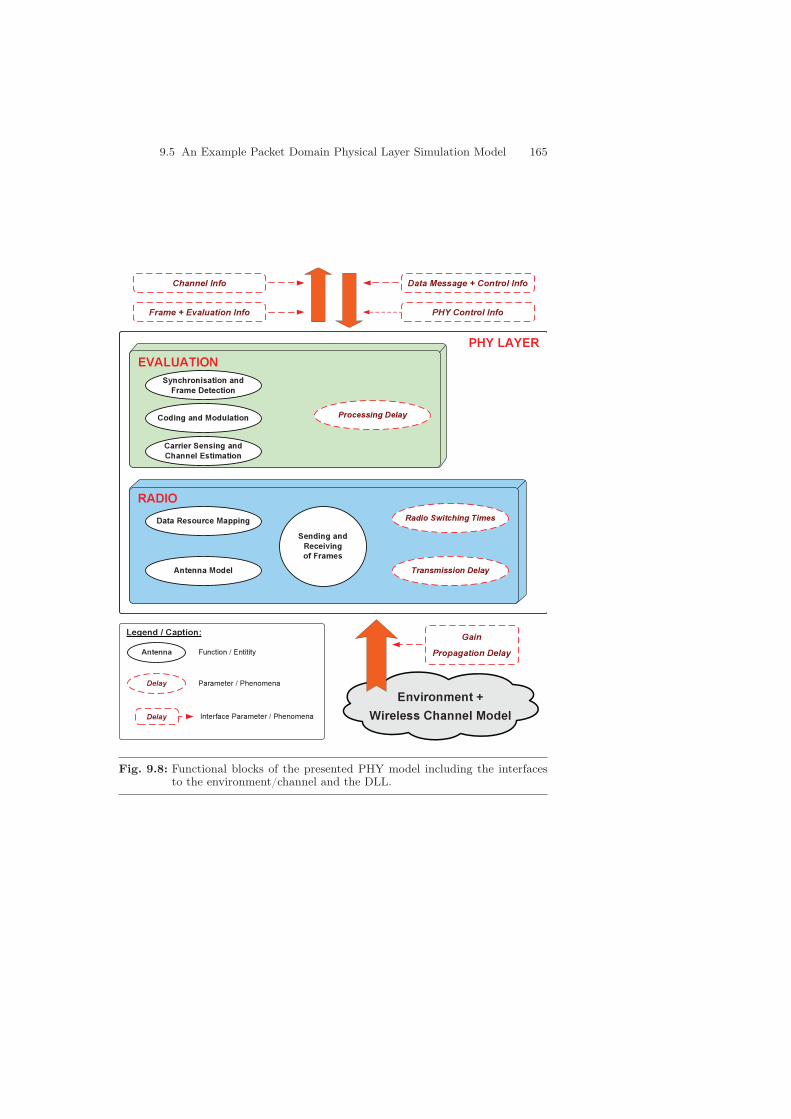
9.5 An Example Packet Domain Physical Layer Simulation Model 165

Environment + Wireless Channel Model

Legend / Caption:

Data Resource Mapping

Antenna Model

Sending and Receiving of Frames

Radio Switching Times

Transmission Delay

Antenna Function / Entitity

Delay Parameter / Phenomena

GainPropagation Delay

Delay Interface Parameter / Phenomena

Data Message + Control Info

PHY Control Info

Synchronisation and Frame Detection

Coding and Modulation

Carrier Sensing and Channel Estimation

Processing Delay

Channel Info

Frame + Evaluation Info

EVALUATIONPHY LAYER

RADIO

Fig. 9.8: Functional blocks of the presented PHY model including the interfacesto the environment/channel and the DLL.


state = send &&

no msg being sent

add resource mapping

meta data

add antenna properties

meta data

msg to environment

yes

msg from DLL

noerror

add position vector

data resource mapping

antenna model

DLL msg + mapping

DLL msg + mapping

+ TX antenna

DLL msg + mapping

+ TX antenna + position

DLL msg

sending

DLL msg

delay (end of msg)

inform DLL

Fig. 9.9: Sending process


As mentioned earlier, the detailed effects of FEC coding and interleavingare modeled by bit-true simulation models on the bit-, symbol-, or sampledomain (see Section 9.2 & 9.3). For packet domain simulations, the impactof coding and interleaving are not considered per bit, but evaluated in com-bination with the chosen modulation scheme as well as other transmissionparameters (cf. Section 9.4.1). As all this information has to be processed atthe receiver, meta data is added to the transmitted frame which contains allinformation that the receiver needs to accurately determine the reception ofthe frame. Appending all information regarding the transmission parametersis done in the Data Resource Mapping block. In addition to typical transmit-ter settings (like modulation and coding type or transmit power), also furtherscheduling decisions regarding the used resources have to be appended likethe used sub channels in OFDMA systems or the used spatial streams inmultiple antenna systems, see Section 10.1.5. Finally, information is addedregarding the used antenna type and its impact on the transmit power, seeSection 11.11.

The frame with its meta data is then passed to the environment (whichmodels the channel including interference effects among other elements, cf.Chapter 11). The environment is responsible for delivering the frame to theappropriate receiving entities. Since the wireless medium is a broadcast chan-nel, there might be more entities than the specified receiver of the frame. Inorder to correctly calculate the channel gain at the moment of the framearrival at the receiver, the transmitter additionally needs to provide its mo-mentary position, speed and direction of movement (referred to as a positionvector) to the environment. Before passing the frame to the environment, thesending and receiving block thus attaches the position vector as meta datato the frame.

Since in simulation the whole frame is “sent” at once, the TransmissionDelay has to be modeled explicitly, i.e. the time between sending of the firstand the last bit of the frame. This is usually done by some delay process. Oncethe last bit of the frame is sent, the PHY has to inform the DLL, so thatit can take appropriate actions (e.g. sending the next message or switchingthe radio back into the receive or sleep state). A state diagram for the wholesending process is shown in Figure 9.9.

Data Resource Mapping. The task of this functional block is to map thedata for transmission on the system resources as determined by a resourcemanager (see Section 10.1.5). However, since we do not consider a bit-truemodel, only PHY frames with an attachment of meta data are considered.The meta data is necessary for the receiving entity to be able to processthe transmitted frame. It comprises the transmission power that is reflectedby the RSSI in a real system. In adaptive modulation and coding systems,the selected parameters for modulation and coding need also be attachedin order to enable the receiver to correctly evaluate the transmitted data. In


multi-carrier and/or multi-antenna systems, this information is necessary percarrier/antenna.

The decision on these transmission parameters is made at the transmitterby the DLL and then passed as control info to the PHY layer via the DLL-PHY interface. An example for a complete set of parameters in a MIMOmulti-carrier transmission system can be the following: “use sub-bands 4, 6,and 8 for transmission on antenna 2: use QPSK and 100 mW on sub-band 4,QPSK and 50 mW on sub-band 6, and 64-QAM and 200 mW on sub-band8.”

Receiving Frames. The received analog signal is attenuated and distortedby the environment it traveled through on its way from the transmitter tothe receiver. Depending on the modeled system, the distortion has to becalculated for different subcarriers, antennas, and once or multiple times perframe in the time domain. These effects are described in detail in Chapter 11.In order to calculate the distortions, the position vector of the receiver (aswell as of the transmitter) is required. All this information is appended to theframe’s meta data before it is delivered to the receiver’s PHY. The details ofthe receiving process are shown in Figure 9.10 and described in the following.

The decision whether an entity is able to receive a frame or not dependson several parameters. First, its radio has to be in receive mode. Second, onlyone frame can be received at a time. Thus, if the PHY is currently in theprocess of receiving a frame, all other frames arriving at that time will betreated as noise (and added to the “noise messages” as shown in Figure 9.10).Alternatively, the receiver might also lock to the strongest signal received,even if it arrives later than some other frame (capturing effect). Which frameto receive and which to treat as noise is determined by the synchronizationand frame detection block. Once the frame is received, bit errors have to becalculated according to some link-to-system interface.

9.5.2 Evaluation Unit

Synchronization and Frame Detection. For each frame arriving at the PHYlayer, the receiver has to decide whether to receive it or treat it as noise. Thepoint in time for the decision (denoted as t1 in Figure 9.10) depends on thechosen model. One possibility is to make the decision immediately after thepacket’s arrival (t1 = 0). This is useful if only a single channel gain value ispresent for the whole frame. Another possibility is to decide at a later time,e.g. after the preamble or header is received and there is at least one channelgain value corresponding to the preamble transmission. The decision whetherto receive the frame or treat it as noise is based on the channel gain and othertransmissions currently ongoing on the medium. The PHY has to derive the


msg from environment

add antenna properties

meta data

antenna model

compute transmission delay

compute SINR matrix

until t1

noise?

compute SINR matrix

until t2

delay t1

delay (t2 - t1)

DLL msg + mapping

+ TX antenna + attenuation

DLL msg + mapping + TX antenna

+ attenuation + RX antenna

no

yes

frame detection

noise messages

compute bit-error

probability

transmission error

analysis

DLL msg + bit-error prob.

msg to DLL

receiving

yes

nostate = receive &&

no msg being received

add to

noise messages

Fig. 9.10: Receiving process


SINR values for the frame or the part of the frame it has already received. Ifdesired, this is also the place to model capturing effects, as mentioned above.

If the message is treated as noise, it is added to the noise power. If not, ithas to be delayed until the end of the frame (t2) and passed to the resourcede-mapping, demodulation, and decoding functional block, which calculatesthe bit-error probability and passes the message to the DLL.

An example is shown in Figure 9.11. Here we assume, that a frame isreceived, if its header can be decoded. In this case “msg2” is the messagebeing evaluated. At the start of receiving “msg2” there has already been“msg1” on the channel, which is assumed to be treated as noise. At time t1,the header of “msg2” is completely received. In order to evaluate the SINRat this point, all interfering messages have to be considered. In Figure 9.11these are “msg1” and “msg3” – “msg4” does not intersect with the header andthus is not of interest. Later, at time t2, also “msg4” is of interest to calculatethe bit errors as described in the Demodulation, and Decoding sub-section.

Fig. 9.11: Receiving of multiple messages

The attached channel gain ℎ2 and transmission power values Ptx of theframe in question (“msg2”) and the corresponding values of the interferinggains ℎ2

j and the interfering transmit powers P Ij of all intersecting frames i

(“msg1” and “msg3”), as well as the noise �2 are used to calculate the SINRas shown in Equation (9.3).

=Ptx ⋅ ℎ

2

∑∀j P

Ij ⋅ ℎ

2

j + �2(9.3)

Note that in general the SINR is not only a single value, but a matrix ofvalues in frequency (different sub-channels), space (different antennas), andtime (if multiple values are to be considered per frame time or if advancedtransmission schemes are employed).


Channel Estimation. As mentioned above, channel estimation is performedon the one hand at the receiver to better decode the modulation symbols.For a packet domain simulation model, this type of channel estimation is notconsidered but is assumed to function perfectly. On the other hand, chan-nel estimation is required such that the transmitter can adapt transmissionparameters by resource management to the channel state. This type of chan-nel estimation is often considered by packet domain PHY simulation models.One way to model this is to let the environment determine the channel stateat frame transmission analytically, according to the estimation algorithm ap-plied. The resulting channel gains are attached to the frame as meta data(see Figure 9.10). The channel estimation part is modeled by passing the re-ceived channel attenuation values on to the DLL that saves it together witha time stamp and transmitter information for future use. In a Time Divi-sion Duplex (TDD) system, if channel reciprocity can be assumed, the storedchannel state information can be used for transmission parameter adaptation(e.g. power, modulation, coding), once the receiver in turn wants to transmitsomething to the former transmitter. Whenever channel reciprocity cannotbe assumed, e.g. in a Frequency Division Duplex (FDD) system, the receiver’sDLL needs to signal the channel information back to the transmitter in orderto enable it to adapt the transmission parameters in the upcoming slots. Forsignaling the channel state information back to the transmitter an additionalsignaling channel is needed.

Carrier Sensing. Carrier sensing at the transmitter is necessary for partic-ular MAC protocols such as CSMA (like in 802.11, see Section 12.1). Carriersensing is a service provided by the PHY to the DLL. Whenever the MACwants to access the channel, it requests the carrier sensing information fromthe PHY. The carrier sensing functional block then has to provide the chan-nel status information and pass this information via the PHY DLL interface.Based on this information, the MAC decides whether the channel is busy oridle. Possibilities to model carrier sensing range from simply introducing arandom delay (done at the DLL) to explicitly modeling the carrier sensingprocess as described above in Section 9.2.

Depending on the type of carrier sensing, feature detection versus energymeasurement, the PHY either has to calculate the RSSI or evaluate the SINRto determine whether the signal is decodable or not. One option to decide onthe decodability of a frame is to consider either the SINR or the correspondingBER. The calculated value (RSSI, SINR or BER) is then compared to somethreshold in order to decide whether the channel is busy or idle. In addition,the DLL has to specify how long the carrier sensing needs to be performed. Insimulation, it is often assumed that carrier sensing can be done in zero time.In this case the PHY would just evaluate the most recent SINR available. Formore accurate simulations however, the delay for the carrier sensing shouldbe simulated.


Demodulation and Decoding. Coding and modulation have a major impacton the transmission quality of a frame. At the packet domain, this impactcan be accounted for by a link-to-system interface (as explained above) whichtakes the SINR as input and determines an instantaneous BER as output. Ifno detailed description of the coding impact is at hand, a simple coding gaincan be assumed which is added to the SINR of the frame. The calculationof transmission errors is usually done once the frame is completely received(t2). The receiver has to calculate the SINR as described above and shownin Equation (9.3) and Figure 9.11. The SINR is used together with the BERcurves or tables to get the bit-error probabilities for the message: the combi-nation of SINR and indicated modulation/coding choice is taken as an inputfor the table or curve look-up, the error probability is the output (as shownin Table 9.5). The level of detail of the bit-error calculation mainly dependson the number of SINR values available. The simplest model is to only haveone SINR value per frame. More detailed models have multiple values toevaluate multiple sections of the frame. One example is to have one value forthe PHY header which are usually transmitted at a lower modulation to en-sure the correct frame detection, and the payload, respectively. Furthermore,there might be another value to distinguish between the MAC header andthe MAC payload in order to be able to evaluate both of them individually.The PHY payload is passed to the DLL layer via the PHY-DLL interfaceaccompanied by the bit-error probability meta data.

9. Physical Layer Modeling - TU Berlin · 9. Physical Layer Modeling...

Documents

Transcript of 9. Physical Layer Modeling - TU Berlin · 9. Physical Layer Modeling...