9 Network Analysis - School of Physics · Finally, network theorems will be introduced. Network...

Air Washington Electronics – Direct Current

of 61

9 Network Analysis

This work is licensed under the Creative Commons Attribution 3.0 Unported License. To view a copy of this license,

visit http://creativecommons.org/licenses/by/3.0/. Air Washington is an equal opportunity employer/program. Auxiliary aids and services are

available upon request to individuals with disabilities. This workforce solution was funded (100%) by a grant awarded by the U.S. Department

of Labor’s Employment and Training Administration. The solution was created by the grantee and does not necessarily reflect the official

position of the U.S. Department of Labor. The Department of Labor makes no guarantees, warranties, or assurances of any kind, express or

implied, with respect to such information, including any information on linked sites and including, but not limited to, accuracy of the

information or its completeness, timeliness, usefulness, adequacy, continued availability, or ownership. This solution is copyrighted by the

institution that created it. Internal use, by an organization and/or personal use by an individual for non-commercial purposes is permissible. All

other uses require the prior authorization of the copyright owner. Revised: Tuesday, June 17, 2014

http://creativecommons.org/licenses/by/3.0/


of 61

Contents

9 Network Analysis ......................................................................................................................... 1

Network Analysis ............................................................................................................................ 3

Branch Current Method .................................................................................................................. 6

Steps to follow for the “Branch Current” method of analysis: ................................................. 11

Mesh Current Method .................................................................................................................. 12

Steps to follow for the Mesh Current Method ......................................................................... 17

Solving More Complex Circuits ................................................................................................. 18

The Wheatstone Bridge............................................................................................................. 19

Node voltage method ................................................................................................................... 23

Node voltage rules .................................................................................................................... 25

Introduction to Network Theorems .............................................................................................. 26

Millman's Theorem ....................................................................................................................... 26

Superposition Theorem ................................................................................................................ 30

Thevenin's Theorem ..................................................................................................................... 35

Steps to follow for Thevenin’s Theorem ................................................................................... 41

Norton's Theorem ......................................................................................................................... 41

Steps to follow for Norton's Theorem: ..................................................................................... 45

Thevenin-Norton Equivalencies .................................................................................................... 46

Millman's Theorem revisited ........................................................................................................ 47

Network conversions .................................................................................................................... 51

Additional Resources .................................................................................................................... 56

Physics Resources ...................................................................................................................... 56

Video Resources ........................................................................................................................ 56

References .................................................................................................................................... 57

Attributions ................................................................................................................................... 58

Table of Figures ............................................................................................................................. 59


of 61

Network Analysis

Generally speaking, network analysis is any structured technique used to mathematically

analyze a network of interconnected components, or circuit. Quite often the technician will

encounter circuits containing multiple sources of power or component configurations which

defy simplification by series- parallel analysis techniques. In those cases, he or she will be

forced to use other means. This chapter presents a few techniques useful in analyzing such

complex circuits.

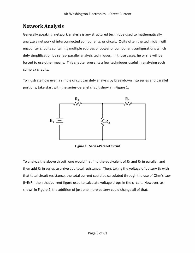
To illustrate how even a simple circuit can defy analysis by breakdown into series and parallel

portions, take start with the series-parallel circuit shown in Figure 1.

To analyze the above circuit, one would first find the equivalent of R2 and R3 in parallel, and

then add R1 in series to arrive at a total resistance. Then, taking the voltage of battery B1 with

that total circuit resistance, the total current could be calculated through the use of Ohm's Law

(I=E/R), then that current figure used to calculate voltage drops in the circuit. However, as

shown in Figure 2, the addition of just one more battery could change all of that.

Figure 1: Series-Parallel Circuit


of 61

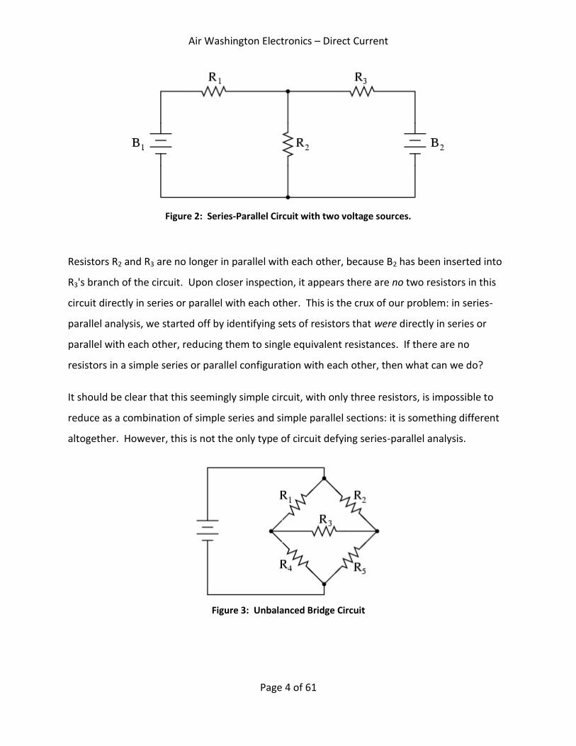
Resistors R2 and R3 are no longer in parallel with each other, because B2 has been inserted into

R3's branch of the circuit. Upon closer inspection, it appears there are no two resistors in this

circuit directly in series or parallel with each other. This is the crux of our problem: in series-

parallel analysis, we started off by identifying sets of resistors that were directly in series or

parallel with each other, reducing them to single equivalent resistances. If there are no

resistors in a simple series or parallel configuration with each other, then what can we do?

It should be clear that this seemingly simple circuit, with only three resistors, is impossible to

reduce as a combination of simple series and simple parallel sections: it is something different

altogether. However, this is not the only type of circuit defying series-parallel analysis.

Figure 2: Series-Parallel Circuit with two voltage sources.

Figure 3: Unbalanced Bridge Circuit


of 61

Figure 3 shows an unbalanced bridge. If it were balanced, there would be zero current through

R3, and it could be approached as a series-parallel combination circuit (R1R4 // R2R5). However,

any current through R3 makes a series-parallel analysis impossible. R1 is not in series with

R4 because there's another path for electrons to flow through R3. Neither is R2 in series with

R5 for the same reason. Likewise, R1 is not in parallel with R2 because R3 is separating their

bottom leads. Neither is R4 in parallel with R5.

Although it might not be apparent at this point, the heart of the problem is the existence of

multiple unknown quantities. At least in a series-parallel combination circuit, there was a way

to find total resistance and total voltage, leaving total current as a single unknown value to

calculate (and then that current was used to satisfy previously unknown variables in the

reduction process until the entire circuit could be analyzed). With these problems, more than

one parameter (variable) is unknown at the most basic level of circuit simplification.

With the two-battery circuit, there is no way to arrive at a value for “total resistance,” because

there are two sources of power to provide voltage and current (we would need two “total”

resistances in order to proceed with any Ohm's Law calculations). With the unbalanced bridge

circuit, there is such a thing as total resistance across the one battery (paving the way for a

calculation of total current), but that total current immediately splits up into unknown

proportions at each end of the bridge, so no further Ohm's Law calculations for voltage (E=IR)

can be carried out.

So what can we do when we're faced with multiple unknowns in a circuit? The answer is

initially found in a mathematical process known as simultaneous equations or systems of

equations, whereby multiple unknown variables are solved by relating them to each other in

multiple equations. In a scenario with only one unknown, there only needs to be a single

equation to solve for the single unknown, as shown in the list of Ohm’s law derivations below.


of 61

This module discusses various techniques of network analysis that can be used to solve complex

circuits. First, there are several different methods using the Ohm’s and Kirchhoff’s laws, such as

the branch and mesh current method, and the node voltage method. Finally, network

theorems will be introduced. Network theorems, such as Millman’s, Superposition, Thevenin’s,

and Norton’s theorems provide the framework necessary for more specific problem solving

techniques

Branch Current Method

The first and most straightforward network analysis technique is called the branch current

method. In this method, we assume directions of currents in a network, and then write

equations describing their relationships to each other through Kirchhoff's and Ohm's laws.

Once we have one equation for every unknown current, we can solve the simultaneous

equations and determine all currents, and therefore all voltage drops in the network.

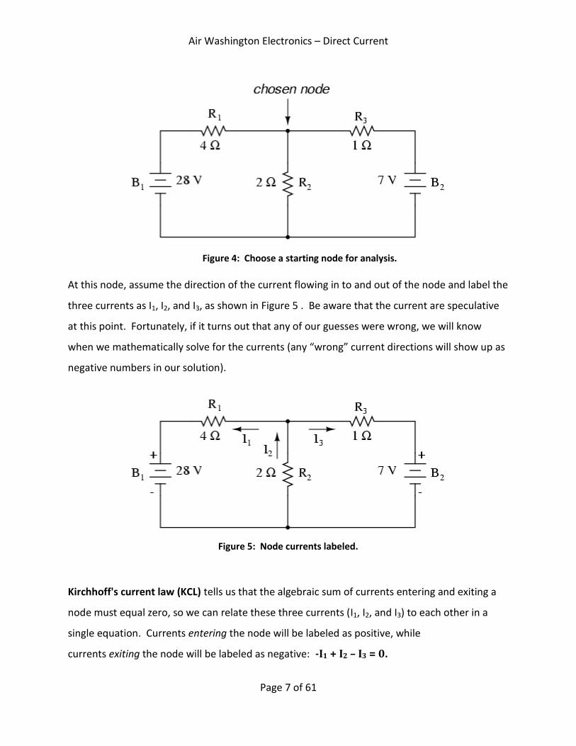
The first step is to choose a node (junction of wires) in the circuit to use as a point of reference

for our unknown currents. Figure 4 indicates the chosen node.


of 61

At this node, assume the direction of the current flowing in to and out of the node and label the

three currents as I1, I2, and I3, as shown in Figure 5 . Be aware that the current are speculative

at this point. Fortunately, if it turns out that any of our guesses were wrong, we will know

when we mathematically solve for the currents (any “wrong” current directions will show up as

negative numbers in our solution).

Kirchhoff's current law (KCL) tells us that the algebraic sum of currents entering and exiting a

node must equal zero, so we can relate these three currents (I1, I2, and I3) to each other in a

single equation. Currents entering the node will be labeled as positive, while

currents exiting the node will be labeled as negative: -I1 + I2 – I3 = 0.

Figure 4: Choose a starting node for analysis.

Figure 5: Node currents labeled.


of 61

The next step is to label all voltage drop polarities across resistors according to the assumed

directions of the currents (Figure 6). Remember that the “upstream” end of a resistor will

always be negative, and the “downstream” end of a resistor positive with respect to each other,

since electrons are negatively charged.

The battery polarities, of course, remain as they were according to the orientation at which

they were drawn. Remember, the short line indicates the negative (or return) side of the

battery and the long line indicates the positive end. It is acceptable if the polarity of a resistor's

voltage drop doesn't match with the polarity of the nearest battery as long as the resistor

voltage polarity is correctly based on the assumed direction of current through it. In some

cases we may discover that current will be forced backwards through a battery, causing this

very effect. The important thing to remember here is to base all your resistor polarities and

subsequent calculations on the assumed directions of current(s). As stated earlier, if your

assumption happens to be incorrect, it will be apparent once the equations have been solved

(by means of a negative solution). The magnitude of the solution, however, will still be correct.

Kirchhoff's voltage law (KVL) states that the algebraic sum of all voltages in a loop must equal

zero. Therefore, we can create more equations with current terms (I1, I2, and I3) for our

simultaneous equations. To obtain a KVL equation, record the voltage drops in each loop of the

Figure 6: Label polarities of voltage drops


of 61

circuit. For the left loop, start at the upper-left corner and move counter-clockwise around the

loop. Upon completion, your equation should look like this: -28 + ER2 + ER1 = 0.

At this point the voltages across R1 or R2 are unknown, but according to KVL, we do know that

all three voltages must algebraically add to zero, so the equation is true. We can go a step

further and express the unknown voltages as the product of the corresponding unknown

currents (I1 and I2) and their respective resistors, following Ohm's Law (E=IR):

Start with: -28 + ER2 + ER1 = 0

Using Ohm’s Law (E = IR), substitute IR for E in the KVL equation: -28 +I2R2 +I1R1 = 0

Since we know what the values of all the resistors are in ohms, we can just substitute

those figures into the equation to simplify things a bit: -28 + 2I2 + 4I1 = 0

You might be wondering why we went through all the trouble of manipulating this equation

from its initial form (-28 + ER2 + ER1 = 0). After all, the last two terms are still unknown, so

what advantage is there to expressing them in terms of unknown voltages or as unknown

currents? The purpose in doing this is to get the KVL equation expressed using the same

unknown variables as the KCL equation, as this is a necessary requirement for any simultaneous

equation solution method. To solve for three unknown currents (I1, I2, and I3), we must have

three equations relating these three currents together.

Applying the same steps to the right loop of the circuit, starting at the chosen node and moving

counter-clockwise, we get another KVL equation: -ER2 + 7 – ER3 = 0.

Knowing now that the voltage across each resistor should be expressed as the product of the

corresponding current and the resistance of each resistor, we can re-write the equation as

such: -2I2 + 7 –I3 = 0


of 61

Now we have a mathematical system of three equations (one KCL equation and two KVL

equations) and three unknowns:

-I1 + I2 – I3 = 0 Kirchhoff’s Current Law

-28 + 2I2 + 4I1 = 0 Kirchhoff’s Voltage Law

-2I2 + 7 – I3 = 0 Kirchhoff’s Voltage Law

For some methods of solution, it is helpful to express each unknown term in each equation,

with any constant value to the right of the equal sign, and with any “unity” terms expressed

with an explicit coefficient of 1. Re-writing the equations again, we have:

-1I1 + 1I2 – 1I3 = 0 Kirchhoff’s Current Law

4I1 + 2I2 + 0I3 = 28 Kirchhoff’s Voltage Law

0I1 – 2I2 – 1I3 = -7 Kirchhoff’s Voltage Law

Using whatever solution techniques are available to us, we should arrive at a solution for the

three unknown current values:

I1 = 5A

I2 = 4A

I3 = -1A

Therefore, I1 is 5 amps, I2 is 4 amps, and I3 is a negative 1 amp. But what does “negative”

current mean? In this case, it means that our assumed direction for I3 was opposite of its real

direction. Going back to our original circuit, we can re-draw the circuit to be in line with what

we have determined (Figure 7).

Solving Simultaneous Equations

All About Circuits

The Math Page

http://www.allaboutcircuits.com/vol_5/chpt_4/11.html

http://www.themathpage.com/alg/simultaneous-equations.htm


of 61

Notice how current is being pushed backwards through battery B2 (electrons flowing from

positive side) due to the higher voltage of battery B1, whose current is flowing from the

negative side. Despite the fact that battery B2's polarity is trying to push electrons down in that

branch of the circuit, electrons are being forced backwards through it due to the superior

voltage of battery B1. Does this mean that the stronger battery will always overpower the

weaker battery and force the current through it backwards? No, because it depends on both

batteries' relative voltages and the resistor values in the circuit. The only way to determine

what is going on is to take the time to mathematically analyze the network.

Now that we know the magnitude of all currents in this circuit, we can calculate voltage drops

across all resistors with Ohm's Law (E=IR):

ER1 = I1R1 = (5 A) (4 Ω) = 20 V

ER2 = I2R2 = (4 A) (2 Ω) = 8 V

ER3 = I3R3 = (1 A) (1 Ω) = 1 V

Steps to follow for the “Branch Current” method of analysis:

Choose a node and assume directions of currents.

Write a KCL equation relating currents at the node.

Figure 7: Redrawn with correct polarities.


of 61

Label resistor voltage drop polarities based on assumed currents.

Write KVL equations for each loop of the circuit, substituting the product IR for E in each

resistor term of the equations.

Solve for unknown branch currents (simultaneous equations).

If any solution is negative, then the assumed direction of current for that solution is

wrong!

Solve for voltage drops across all resistors (E=IR).

Mesh Current Method

The mesh current method also known as the loop current method is quite similar to the branch

current method in that it uses simultaneous equations, Kirchhoff's voltage law, and Ohm's law

to determine unknown currents in a network. It differs from the branch current method in that

it does not use Kirchhoff's current law, and it is usually able to solve a circuit with less unknown

variables and less simultaneous equations, which is especially nice if you are forced to solve

without a calculator.

Figure 8: Series-Parallel Circuit to be analyzed.


of 61

The circuit (Figure 8) used for this example is the same as the one used for the branch current

method. The first step in the mesh current method is to identify loops within the circuit

encompassing all components. In our example circuit, the loop formed by B1, R1, and R2 will be

the first while the loop formed by B2, R2, and R3 will be the second (Figure 9).

The choice of each current's direction is entirely arbitrary, just as in the branch current method,

but the resulting equations are easier to solve if the currents are going the same direction

through intersecting components. In the figure above, note how currents I1 and I2 are both

flowing up through resistor R2, where they mesh, or intersect. As with the branch current

method, if the assumed direction of a mesh current is wrong, the answer for that current will

have a negative value.

The next step is to label all voltage drop polarities across resistors according to the assumed

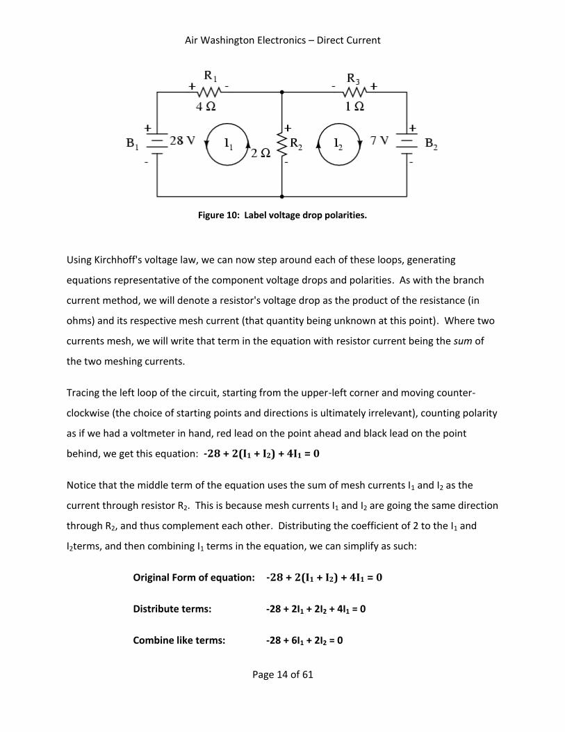
directions of the mesh currents as shown in Figure 10. Remember that the “upstream” end of a

resistor will always be negative, and the “downstream” end of a resistor positive with respect

to each other, since electrons are negatively charged. The battery polarities, of course, are

dictated by their symbol orientations in the diagram, and may or may not “agree” with the

resistor polarities (assumed current directions).

Figure 9: Identify loops in each part of the mesh.


of 61

Using Kirchhoff's voltage law, we can now step around each of these loops, generating

equations representative of the component voltage drops and polarities. As with the branch

current method, we will denote a resistor's voltage drop as the product of the resistance (in

ohms) and its respective mesh current (that quantity being unknown at this point). Where two

currents mesh, we will write that term in the equation with resistor current being the sum of

the two meshing currents.

Tracing the left loop of the circuit, starting from the upper-left corner and moving counter-

clockwise (the choice of starting points and directions is ultimately irrelevant), counting polarity

as if we had a voltmeter in hand, red lead on the point ahead and black lead on the point

behind, we get this equation: -28 + 2(I1 + I2) + 4I1 = 0

Notice that the middle term of the equation uses the sum of mesh currents I1 and I2 as the

current through resistor R2. This is because mesh currents I1 and I2 are going the same direction

through R2, and thus complement each other. Distributing the coefficient of 2 to the I1 and

I2terms, and then combining I1 terms in the equation, we can simplify as such:

Original Form of equation: -28 + 2(I1 + I2) + 4I1 = 0

Distribute terms: -28 + 2I1 + 2I2 + 4I1 = 0

Combine like terms: -28 + 6I1 + 2I2 = 0

Figure 10: Label voltage drop polarities.


of 61

At this time we have one equation with two unknowns. To be able to solve for two unknown

mesh currents, we must have two equations. If we trace the other loop of the circuit, we can

obtain another KVL equation and have enough data to solve for the two currents.

Starting at the upper-left hand corner of the right loop and tracing counter-clockwise:

-2(I1 + I2) + 7 -1I2 = 0

Simplify the equation as before:

-2I1 – 3I2 + 7 = 0

Now, with two equations, we can use one of several methods to solve for the unknown

currents I1 and I2:

-28 + 6I1 + 2I2 = 0

-2I1 – 3I2 + 7 = 0

Rearrange equations for easier solution:

6I1 + 2I2 = 28

-2I1 – 3I2 = -7

Solutions:

I1 = 5 A

I2 = -1 A

Knowing that these solutions are values for mesh currents, not branch currents, we must return

to our diagram to see how they fit together to give currents through all components as shown

in Figure 11.


of 61

The solution of -1 amp for I2 means that our initially assumed direction of current was incorrect.

In actuality, I2 is flowing in a counter-clockwise direction at a value of (positive) 1 amp as shown

in Figure 12.

This change of current direction from what was first assumed will alter the polarity of the

voltage drops across R2 and R3 due to current I2. From here, we can say that the current

through R1 is 5 amps, with the voltage drop across R1 being the product of current and

resistance (E=IR), 20 volts (positive on the left and negative on the right). Also, we can safely

say that the current through R3 is 1 amp, with a voltage drop of 1 volt (E=IR), positive on the left

and negative on the right. However, what is happening at R2?

Figure 11: Original current directions for each mesh.

Figure 12: Corrected current directions for I2.


of 61

Mesh current I1 is going “up” through R2, while mesh current I2 is going “down” through R2. To

determine the actual current through R2, we must see how mesh currents I1 and I2 interact (in

this case they're in opposition), and algebraically add them to arrive at a final value. Since I1 is

going “up” at 5 amps, and I2 is going “down” at 1 amp, the real current through R2 must be a

value of 4 amps, going “up” (Figure 13).

A current of 4 amps through R2's resistance of 2 Ω gives us a voltage drop of 8 volts (E=IR),

positive on the top and negative on the bottom.

Steps to follow for the Mesh Current Method

Draw mesh currents in loops of circuit, enough to account for all components.

Label resistor voltage drop polarities based on assumed directions of mesh currents.

Write KVL equations for each loop of the circuit, substituting the product IR for E in each

resistor term of the equation. Where two mesh currents intersect through a

component, express the current as the algebraic sum of those two mesh currents (i.e.

I1 + I2) if the currents go in the same direction through that component. If not, express

the current as the difference (i.e. I1 - I2).

Solve for unknown mesh currents (simultaneous equations).

If any solution is negative, then the assumed current direction is wrong!

Figure 13: Direction of current flow.


of 61

Algebraically add mesh currents to find current in components sharing multiple mesh

currents.

Solve for voltage drops across all resistors (E=IR).

Solving More Complex Circuits

The primary advantage of mesh current analysis is that it generally allows for the solution of a

large network with fewer unknown values and fewer simultaneous equations. The previous

example problem took three equations to solve using the branch current method and only two

equations using the mesh current method. For more complex networks (Figure 14) the

advantage afforded by mesh current analysis becomes evident.

To solve this network using branch currents, five variables would need to be used to account

for each unique current in the circuit (Figure 15).

Figure 15: Solving a complex series-parallel circuit using branch current method.

-I1 + I2 + I3 = 0 KCL at node 1

-I3 + I4 – I5 = 0 KCL at node 2

-EB1 + I2R2 + I1R1 = 0 KVL in left loop

-I2R2 + I4R4 + I3R3 = 0 KVL in center loop

-I4R4 + EB2 – I5R5 = 0 KVL in right loop

Figure 14: Complex series-parallel circuit with multiple batteries.


of 61

As shown in Figure 16, the mesh current method is a more effective choice, requiring only three

unknowns and three equations to solve. Working with fewer equations is an advantage,

especially when performing simultaneous equation solution by hand without a calculator.

KVL in left loop

-EB1 + R2(I1 + I2) + I1R1 = 0

KVL in center loop

-R2(I2 + I1) – R4(I2 + I3) – I2R3 = 0

KVL in right loop

R4(I3 + I2) + EB2 + I3+R5 = 0

Figure 16: Solving a complex series-parallel circuit using mesh current method.

The Wheatstone Bridge

Another type of circuit that lends itself well to mesh current method is the unbalanced

Wheatstone bridge as shown in Figure 17.

Figure 17: Unbalanced Wheatstone bridge circuit.


of 61

Because the ratios of R1 to R4 and R2 to R5 are unequal, there will be voltage across resistor R3,

and some amount of current through it. As discussed at the beginning of this module, this type

of circuit is irreducible by normal series-parallel analysis, and may only be analyzed by some

other method.

The branch current method would require a large set of simultaneous equations due to the

multiple (six) current paths. The mesh current method, however, provides a less complicated

means for solving this and other complicated circuits. The first step in the mesh current

method is to draw the currents in each mesh section, or loop. The placement of the first two

currents should be obvious, as shown below.

As previously discussed, the initial directions of these mesh currents is arbitrary. However, two

mesh currents are not enough in this circuit, because neither I1 nor I2 goes through the battery.

Therefore, a third mesh current, I3, needs to be added.

Figure 18: Drawing mesh currents in an unbalanced bridge.


of 61

In Figure 19, I3 loops from the bottom side of the battery, through R4, through R1, and back to

the top side of the battery. This is not the only path available for I3, but it is the simplest. With

the mesh currents identified, label the polarity of the voltage drops across each resistor,

following each of the assumed currents' directions.

Notice something very important here: at resistor R4, the polarities for the respective mesh

currents do not agree. This is because those mesh currents (I2 and I3) are going through R4 in

different directions. While this does not preclude the use of the mesh current method for

analysis, it does complicate it.

Generating a KVL equation for the top loop of the bridge, start at the top node and trace

in a clockwise direction: 50I1 + 100(I1 + I2) +150(I1 + I3) = 0

Distribute terms: 50I1 + 100I1 + 100I2 + 150I1 + 150I3 = 0

Combine like terms: 300I1 + 100I2 + 150I3 = 0

Figure 19: Mesh currents and voltage polarities.


of 61

In this equation, the common directions of currents are represented by their sums through

common resistors. For example, resistor R3, with a value of 100 Ω, has its voltage drop

represented in the above KVL equation by the expression 100(I1 + I2), since both currents I1 and

I2 go through R3from right to left. The same exists for resistor R1, with its voltage drop

expression shown as 150(I1 + I3), since both I1 and I3 go from bottom to top through that

resistor, and thus work together to generate its voltage drop.

Starting at the right-hand node, trace counter-clockwise:

100(I1 + I2) + 300(I2 – I3) + 250I2 = 0

Distribute terms: 100I1 + 100I2 + 300I2 – 300I3 + 250I2 = 0

Combine like terms: 100I1 + 650I2 – 300I3 = 0

Note how the second term in the equation's original form has resistor R4's value of 300 Ω

multiplied by the difference between I2 and I3 (I2 - I3). This is how we represent the combined

effect of two mesh currents going in opposite directions through the same component.

Choosing the appropriate mathematical signs is very important here: 300(I2 - I3) does not mean

the same thing as 300(I3 - I2).

The third equation must include the battery's voltage, which up to this point does not appear in

either of the previous KVL equations.

Trace a loop starting from the battery's bottom (negative) terminal, stepping clockwise:

24 – 150(I3 + I1) – 300(I3 – I2) = 0

Distribute terms: 24 – 150I3 – 150I1 – 300I3 + 300I2 = 0

Combine terms: -150I1 + 300I2 – 450I3 = -24

We now have the equations necessary to solve this circuit:


of 61

Solution: I1 = -93.793 mA

I2 = 77.241 mA

I3 = 136.092 mA

Node voltage method

The node voltage method of analysis solves for unknown voltages at circuit nodes in terms of a

system of KCL equations. This analysis involves replacing voltage sources with equivalent

current sources. Also, resistor values in ohms are replaced by equivalent conductances in

siemens (S), G = 1/R.

Start with a circuit having conventional voltage sources. A common node E0 is chosen as a

reference point. The node voltages E1 and E2 are calculated with respect to this point.

A voltage source in series with a resistance must be replaced by an equivalent current source in

parallel with the resistance. Write KCL equations for each node. The right hand side of the

equation is the value of the current source feeding the node. The symbol for a current source is

a circle with an arrow pointing downwards. Please note that this is a convention and does not

indicate current direction.

Top loop of bridge 300I1 + 100I2 + 150I3 = 0

Bottom loop of bridge 100I1 + 650I2 – 300I3 = 0

Bottom loop, including battery -150I1 + 300I2 – 450I3 = -2

Figure 20: Node voltage method for solving circuit unknowns


of 61

Replacing voltage sources and associated series resistors with equivalent current sources and

parallel resistors yields the modified circuit. Substitute resistor conductances in siemens for

resistance in ohms.

Calculate current sources for B1 and B2:

I1 = E1/R1 = 10/2 = 5 A

I2 = E2/R5 = 4/1 = 4 A

Calculate conductance of each resistor:

G1 = 1/R1 = 1/2 Ω = 0.5 S

G2 = 1/R2 = 1/4 Ω = 0.25 S

G3 = 1/R3 = 1/2.5 Ω = 0.4 S

G4 = 1/R4 = 1/5 Ω = 0.2 S

G5 = 1/R5 = 1/1 Ω = 1.0 S

Figure 21: Replacing voltage source with source current.

Figure 22: Circuit with current sources and conductances


of 61

The Parallel conductances (resistors) may be combined by addition of the conductances.

Though, we will not redraw the circuit. The circuit is ready for application of the node voltage

method.

GA = G1 + G2 = 0.5 S + 0.25 S = 0.75 S

GB = G4 + G5 = 0.2 S + 1 S = 1.2 S

Deriving a general node voltage method, write a pair of KCL equations in terms of unknown

node voltages V1 and V2 this one time. This is done to illustrate a pattern for writing equations

by inspection.

GAE1 + G3 (E1 - E2) = I1 (1)

GBE2 - G3 (E1 - E2) = I2 (2)

(GA + G3) E1 -G3E2 = I1 (1)

-G3E1 + (GB + G3) E2 = I2 (2)

The coefficients of the last pair of equations above have been rearranged to show a pattern.

The sum of conductances connected to the first node is the positive coefficient of the first

voltage in equation (1). The sum of conductances connected to the second node is the positive

coefficient of the second voltage in equation (2). The other coefficients are negative,

representing conductances between nodes. For both equations, the right hand side is equal to

the respective current source connected to the node. This pattern allows us to quickly write

the equations by inspection. This leads to a set of rules for the node voltage method of

analysis.

Node voltage rules

1. Convert voltage sources in series with a resistor to an equivalent current source with the

resistor in parallel.

2. Change resistor values to conductances.

3. Select a reference node(E0)


of 61

4. Assign unknown voltages (E1) (E2) ... (EN) to remaining nodes.

5. Write a KCL equation for each node 1, 2, ... N. The positive coefficient of the first

voltage in the first equation is the sum of conductances connected to the node. The

coefficient for the second voltage in the second equation is the sum of conductances

connected to that node. Repeat for coefficient of third voltage, third equation, and

other equations. These coefficients fall on a diagonal.

6. All other coefficients for all equations are negative, representing conductances between

nodes. The first equation, second coefficient is the conductance from node 1 to node 2;

the third coefficient is the conductance from node 1 to node 3. Fill in negative

coefficients for other equations.

7. The right hand side of the equations is the current source connected to the respective

nodes.

8. Solve system of equations for unknown node voltages.

Introduction to Network Theorems

A theorem is a relatively simple rule used to solve a problem and is derived from a more

intensive analysis using fundamental rules of mathematics. In electric network analysis, the

fundamental rules are Ohm's law and Kirchhoff's laws. While these laws may be applied to

analyze nearly any circuit configuration, there are some shortcut methods of analysis to make

the math more manageable.

As with any theorem of algebra, these network theorems are derived from fundamental rules.

In this module, the formal proofs of these theorems will not be presented, however, if desired,

you can empirically test them by setting up example circuits and calculating values using the

simultaneous equation method versus the theorems, to see if the answers coincide.

Millman's Theorem

In Millman's theorem, the circuit is re-drawn as a parallel network of branches, each branch

containing a resistor or series battery-resistor combination. Millman's theorem is applicable

only to those circuits which can be re-drawn accordingly. Here again is the example circuit used

for the previous methods of analysis, but re-drawn for the sake of applying Millman's theorem.


of 61

By considering the supply voltage within each branch and the resistance within each branch,

Millman's theorem will tell us the voltage across all branches. Please note the battery in the

rightmost branch is labeled as “B3” to clearly denote it as being in the third branch, even though

there is no “B2” in the circuit.

Millman's theorem is nothing more than a long equation, applied to any circuit drawn as a set

of parallel-connected branches with each branch having its own voltage source and series

resistance.

Substituting actual voltage and resistance figures from our example circuit for the variable

terms of this equation, we get the following expression:

Figure 23: Series-parallel circuit redrawn for Millman’s theorem.

Figure 24: Millman’s theorem equation.


of 61

The final answer of 8 volts is the voltage seen across all parallel branches, like this:

The polarities of all voltages in Millman’s theorem are referenced to the same point. In the

example circuit above, the bottom wire of the parallel circuit is the reference point; therefore,

the voltages within each branch (28 for the R1 branch, 0 for the R2 branch, and 7 for the R3

branch) were inserted into the equation as positive numbers. Likewise, when the answer came

out to 8 volts (positive), this meant that the top wire of the circuit was positive with respect to

the bottom wire (the original point of reference). If both batteries had been connected

backwards (negative ends up and positive ends down), the voltage for branch 1 would have

been entered into the equation as a -28 volts, the voltage for branch 3 as -7 volts, and the

resulting answer of -8 volts would have indicated that the top wire was negative with respect to

the bottom wire (the initial point of reference).

Figure 25: Millman’s theorem equation for sample circuit.

Figure 26: Circuit voltages redrawn according to Millman’s theorem.


of 61

To solve for resistor voltage drops, the Millman voltage (across the parallel network) must be

compared against the voltage source within each branch, using the principle of voltages adding

in series to determine the magnitude and polarity of voltage across each resistor:

To solve for branch currents, each resistor voltage drop can be divided by its respective

resistance (I=E/R):

The direction of current through each resistor is determined by the polarity across each

resistor, not by the polarity across each battery, as current can be forced backwards through a

battery, as is the case with B3 in the example circuit. This is important to keep in mind, since

Millman's theorem doesn't provide as direct an indication of “wrong” current direction as does

the branch current or mesh current methods. You must pay close attention to the polarities of

resistor voltage drops as given by Kirchhoff's voltage law, determining direction of currents

from that.

Figure 27: Solving for resistor voltage drops.

Figure 28: Solving for branch currents.


of 61

Millman's theorem is very convenient for determining the voltage across a set of parallel

branches, where there are enough voltage sources present to preclude solution via regular

series-parallel reduction method. It also is easy in the sense that it doesn't require the use of

simultaneous equations. However, it is limited in that it only applied to circuits which can be

re-drawn to fit this form. It cannot be used, for example, to solve an unbalanced bridge circuit.

Even in cases where Millman's theorem can be applied, the solution of individual resistor

voltage drops can be daunting with Millman's theorem equation only providing a single figure

for branch voltage.

Each network analysis method has its own advantages and disadvantages. Each method is a

tool, and no tool is perfect for all jobs. The skilled technician, however, carries these methods

in his or her mind like a mechanic carries a set of tools in his or her tool box. The more tools

you have equipped yourself with, the more prepared you will be for any eventuality.

Superposition Theorem

Superposition theorem takes a complex subject and simplifies it in a way that makes perfect

sense. A theorem like Millman's certainly works well, but it is not quite obvious why it works so

well. Superposition, on the other hand, is obvious.

Figure 29: Polarities and direction of current flow.


of 61

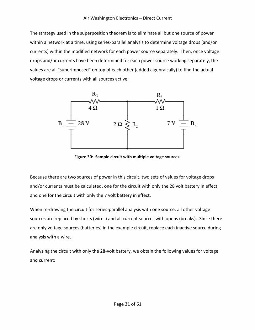
The strategy used in the superposition theorem is to eliminate all but one source of power

within a network at a time, using series-parallel analysis to determine voltage drops (and/or

currents) within the modified network for each power source separately. Then, once voltage

drops and/or currents have been determined for each power source working separately, the

values are all “superimposed” on top of each other (added algebraically) to find the actual

voltage drops or currents with all sources active.

Because there are two sources of power in this circuit, two sets of values for voltage drops

and/or currents must be calculated, one for the circuit with only the 28 volt battery in effect,

and one for the circuit with only the 7 volt battery in effect.

When re-drawing the circuit for series-parallel analysis with one source, all other voltage

sources are replaced by shorts (wires) and all current sources with opens (breaks). Since there

are only voltage sources (batteries) in the example circuit, replace each inactive source during

analysis with a wire.

Analyzing the circuit with only the 28-volt battery, we obtain the following values for voltage

and current:

Figure 30: Sample circuit with multiple voltage sources.


of 61

Analyzing the circuit with only the 7-volt battery, we obtain another set of values for voltage

and current:

Figure 31: Analysis of circuit with 28 V source.

Figure 32: Analysis of circuit with 7 V source.


of 61

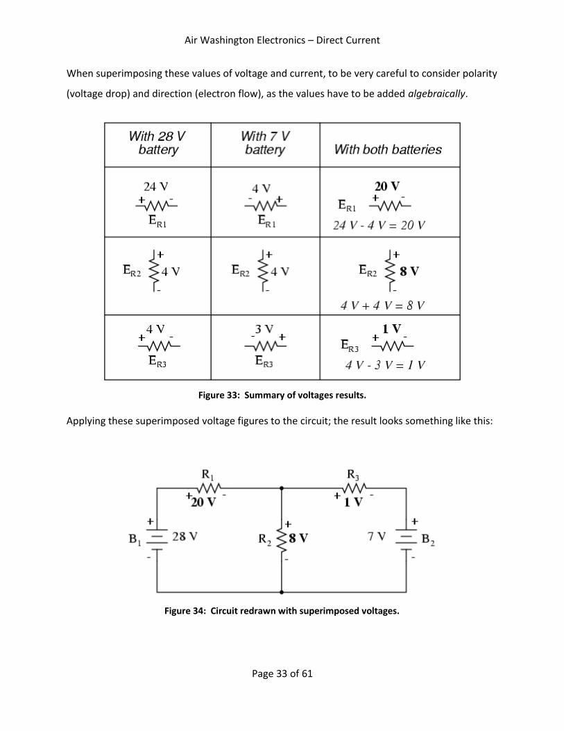
When superimposing these values of voltage and current, to be very careful to consider polarity

(voltage drop) and direction (electron flow), as the values have to be added algebraically.

Applying these superimposed voltage figures to the circuit; the result looks something like this:

Figure 33: Summary of voltages results.

Figure 34: Circuit redrawn with superimposed voltages.


of 61

Currents add up algebraically as well, and can either be superimposed as done with the resistor

voltage drops, or simply calculated from the final voltage drops and respective resistances

(I=E/R). Either way, the answers will be the same.

Here is the superposition method as applied to current:

Once again applying these superimposed figures to the circuit:

Figure 35: Summary of current results

Figure 36: Circuit redrawn with superimposed currents.


of 61

It must be noted, though, that the superposition theorem works only for circuits that are

reducible to series-parallel combinations for each of the power sources at a time and works

only where the underlying equations are linear. The requisite of linearity means that

superposition theorem is only applicable for determining voltage and current, not power.

Power dissipations are nonlinear functions and do not algebraically add to an accurate total

when only one source is considered at a time. The need for linearity also means this theorem

cannot be applied in circuits where the resistance of a component changes with voltage or

current. Hence, networks containing components like lamps (incandescent or gas-discharge) or

varistors could not be analyzed.

Another prerequisite for superposition theorem is that all components must be bilateral,

meaning that they behave the same with electrons flowing either direction through them.

Resistors have no polarity-specific behavior, and so the circuits studied so far all meet this

criterion.

The superposition theorem finds use in the study of alternating current (AC) circuits, and

semiconductor (amplifier) circuits, where sometimes AC is often mixed (superimposed) with

DC. Because AC voltage and current equations (Ohm's law) are linear just like DC, we can use

superposition to analyze the circuit with just the DC power source, and then just the AC power

source, combining the results to tell what will happen with both AC and DC sources in effect.

For now, though, Superposition will suffice as a break from having to do simultaneous

equations to analyze a circuit.

Thevenin's Theorem

Thevenin's theorem states that it is possible to simplify any linear circuit, no matter how

complex, to an equivalent circuit with just a single voltage source and series resistance

connected to a load. The qualification of linearity is identical to that found in the superposition

theorem, where all the underlying equations must be linear (no exponents or roots). If we're

dealing with passive components (such as resistors, and later, inductors and capacitors), this is

true. However, there are some components (especially certain gas-discharge and


of 61

semiconductor components) which are nonlinear: that is, their opposition to

current changes with voltage. As such, we would call circuits containing these types of

components, nonlinear circuits.

Thevenin's theorem is especially useful in analyzing power systems and other circuits where

one particular resistor in the circuit (called the “load” resistor) is subject to change, and re-

calculation of the circuit is necessary with each trial value of load resistance, to determine

voltage across it and current through it. Take another look at our example circuit:

Suppose that we decide to designate R2 as the “load” resistor in this circuit. We already have

four methods of analysis at our disposal (branch current, mesh current, Millman's theorem, and

superposition theorem) to use in determining voltage across R2 and current through R2, but

each of these methods is time-consuming. Imagine repeating any of these methods repeatedly

to find what would happen if the load resistance changed.

Thevenin's theorem makes this easy by temporarily removing the load resistance from the

original circuit and reducing what's left to an equivalent circuit composed of a single voltage

source and series resistance. The load resistance can then be re-connected to this Thevenin

equivalent circuit and calculations carried out as if the whole network were nothing but a

simple series circuit:

Figure 37: Sample series-parallel circuit with multiple voltage sources.


of 61

The Thevenin equivalent circuit is the electrical equivalent of B1, R1, R3, and B2 as seen from the

two points where our load resistor (R2) connects.

The Thevenin equivalent circuit, if correctly derived, will behave exactly the same as the original

circuit formed by B1, R1, R3, and B2. In other words, the load resistor (R2) voltage and current

should be exactly the same for the same value of load resistance in the two circuits. The load

resistor R2 cannot tell the difference between the original network of B1, R1, R3, and B2, and the

Thevenin equivalent circuit of EThevenin, and RThevenin, provided that the values for EThevenin and

RThevenin have been calculated correctly.

Figure 38: Sample circuit redrawn for Thevenin analysis.

Figure 39: Thevenin equivalent of sample circuit.


of 61

Figure 41: Calculate voltage drop of opened load.

The advantage in performing the Thevenin conversion to the simpler circuit, of course, is that it

makes load voltage and load current so much easier to solve than in the original network.

Calculating the equivalent Thevenin source voltage and series resistance is actually quite easy.

First, the chosen load resistor is removed from the original circuit, replaced with a break (open

circuit):

Next, determine the voltage between the two points left by the removal of the load resistor In

this case, the original circuit with the load resistor removed is nothing more than a simple series

circuit with opposing batteries, and so we can determine the voltage across the open load

terminals by applying the rules of series circuits, Ohm's law, and Kirchhoff's voltage law:

Figure 40: Step 1 – Open the load resistor.


of 61

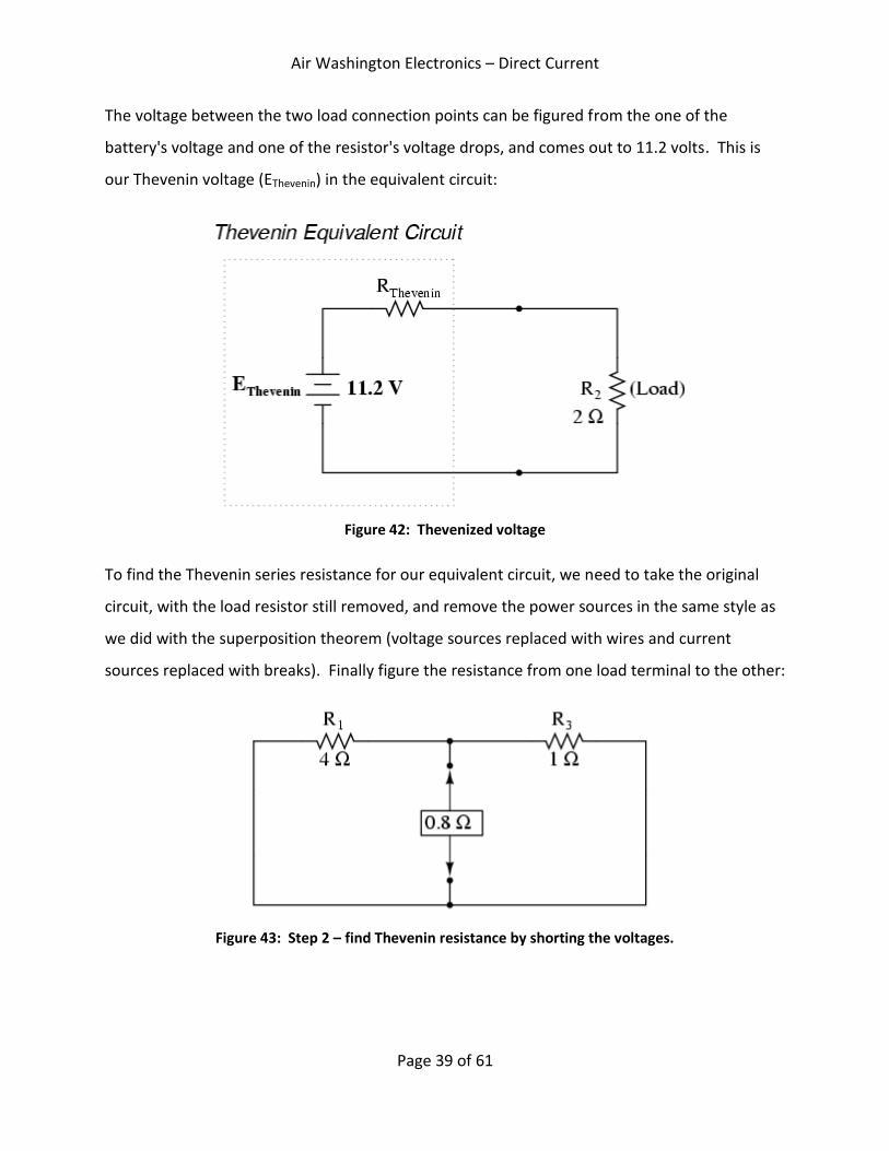
The voltage between the two load connection points can be figured from the one of the

battery's voltage and one of the resistor's voltage drops, and comes out to 11.2 volts. This is

our Thevenin voltage (EThevenin) in the equivalent circuit:

To find the Thevenin series resistance for our equivalent circuit, we need to take the original

circuit, with the load resistor still removed, and remove the power sources in the same style as

we did with the superposition theorem (voltage sources replaced with wires and current

sources replaced with breaks). Finally figure the resistance from one load terminal to the other:

Figure 42: Thevenized voltage

Figure 43: Step 2 – find Thevenin resistance by shorting the voltages.


of 61

With the removal of the two batteries, the total resistance measured at this location is equal to

R1 and R3 in parallel: 0.8 Ω. This is our Thevenin resistance (RThevenin) for the equivalent circuit:

With the load resistor (2 Ω) attached between the connection points, determine the voltage

across it and current through it as though the whole network were nothing more than a simple

series circuit:

Notice that the voltage and current figures for R2 (8 volts, 4 amps) are identical to those found

using other methods of analysis. Also notice that the voltage and current figures for the

Thevenin series resistance and the Thevenin source (total) do not apply to any component in

the original, complex circuit. Thevenin's theorem is only useful for determining what happens

to a single resistor in a network, the load.

Figure 44: Step 3 Draw the Thevenin circuit.

Figure 45: Step 4 – Analyze voltage and current for RLoad


of 61

The advantage, of course, is that it can be quickly determined what would happen to that single

resistor if it were to change.

Steps to follow for Thevenin’s Theorem

1. Find the Thevenin source voltage by removing the load resistor from the original circuit

and calculating voltage across the open connection points where the load resistor used

to be.

2. Find the Thevenin resistance by removing all power sources in the original circuit

(voltage sources shorted and current sources open) and calculating total resistance

between the open connection points.

3. Draw the Thevenin equivalent circuit, with the Thevenin voltage source in series with

the Thevenin resistance. The load resistor re-attaches between the two open points of

the equivalent circuit.

4. Analyze voltage and current for the load resistor following the rules for series circuits.

Norton's Theorem

Norton's Theorem states that it is possible to simplify any linear circuit, no matter how

complex, to an equivalent circuit with just a single current source and parallel resistance

connected to a load. Just as with Thevenin's theorem all underlying equations must be linear.

Before Norton conversion, the original example circuit looks like this:

Figure 46: Sample circuit before Norton conversion.


of 61

After Norton conversion, the equivalent circuit looks like this:

Remember that a current source is a component whose job is to provide a constant amount of

current, outputting as much or as little voltage necessary to maintain that constant current.

As with Thevenin's theorem, everything in the original circuit except the load resistance has

been reduced to an equivalent circuit that is simpler to analyze. Also similar to Thevenin's

theorem are the steps used in Norton's theorem to calculate the Norton source current (INorton)

and Norton resistance (RNorton).

As before, the first step is to identify the load resistance and remove it from the original circuit:

Figure 47: Sample circuit after Norton conversion.

Figure 48: Step 1A – Identify and remove the load resistance.


of 61

Then, to find the Norton current (for the current source in the Norton equivalent circuit), place

a direct wire (short) connection between the load points, and determine the resultant current.

Note that this step is exactly opposite the respective step in Thevenin's theorem, where we

replaced the load resistor with a break (open circuit):

With zero voltage dropped between the load resistor connection points, the current through

R1 is strictly a function of B1's voltage and R1's resistance: 7 amps (I=E/R). Likewise, the current

through R3 is now strictly a function of B2's voltage and R3's resistance: 7 amps (I=E/R). The

total current through the short between the load connection points is the sum of these two

currents: 7 amps + 7 amps = 14 amps. This figure of 14 amps becomes the Norton source

current (INorton) in our equivalent circuit:

Figure 49: Step 1B – Replace the connection with a wire (Short).

Figure 50: Norton equivalent circuit.


of 61

Remember, the symbol for a current source is standardized and does not reflect the direction

of current flow.

To calculate the Norton resistance (RNorton), follow the exact same process as for calculating

Thevenin resistance (RThevenin). Starting with the original circuit, with the load resistor still

removed, and remove the power sources in the same style as with the Superposition theorem.

Finally figure total resistance from one load connection point to the other:

The Norton equivalent circuit of the original circuit now looks like this:

Figure 51: Step 2 - find Norton resistance by shorting the voltages and opening the current sources.

Figure 52: Step 3 – Draw the Norton equivalent circuit.


of 61

Reconnect the original load resistance of 2 Ω, and analyze the Norton circuit as a simple parallel

arrangement:

As with the Thevenin equivalent circuit, the only useful information from this analysis is the

voltage and current values for R2; the rest of the information is irrelevant to the original circuit.

However, the same advantages as with Thevenin's theorem apply to Norton's as well, allowing

for analysis to be performed on changing conditions.

Steps to follow for Norton's Theorem:

1. Find the Norton source current by removing the load resistor from the original circuit

and calculating current through a short (wire) jumping across the open connection

points where the load resistor used to be.

2. Find the Norton resistance by removing all power sources in the original circuit (voltage

sources shorted and current sources open) and calculating total resistance between the

open connection points.

3. Draw the Norton equivalent circuit, with the Norton current source in parallel with the

Norton resistance. The load resistor re-attaches between the two open points of the

equivalent circuit.

4. Analyze voltage and current for the load resistor following the rules for parallel circuits.

Figure 53: Step 4 – Analyze voltage and current for RLoad


of 61

Thevenin-Norton Equivalencies

Since Thevenin's and Norton's theorems are two equally valid methods of reducing a complex

network down to something simpler to analyze, there must be some way to convert a Thevenin

equivalent circuit to a Norton equivalent circuit, and vice versa.

Notice that the procedure for calculating Thevenin resistance is identical to the procedure for

calculating Norton resistance: remove all power sources and determine resistance between the

open load connection points. As such, Thevenin and Norton resistances for the same original

network must be equal. Using the example circuits from the last two sections, we can see that

the two resistances are indeed equal and therefore, RThevenin = RNorton.

Figure 54: Thevenin and Norton equivalent circuits.

Considering the fact that both Thevenin and Norton equivalent circuits are intended to behave

the same as the original network in supplying voltage and current to the load resistor (as seen

from the perspective of the load connection points), these two equivalent circuits, having been

derived from the same original network should behave identically.

This means that both Thevenin and Norton equivalent circuits should produce the same voltage

across the load terminals with no load resistor attached. With the Thevenin equivalent, the

open-circuited voltage would be equal to the Thevenin source voltage (no circuit current

present to drop voltage across the series resistor), which is 11.2 volts in this case. With the

Norton equivalent circuit, all 14 amps from the Norton current source would have to flow

through the 0.8 Ω Norton resistance, producing the exact same voltage, 11.2 volts (E=IR). Thus,


of 61

we can say that the Thevenin voltage is equal to the Norton current times the Norton

resistance: EThevenin = INortonRNorton

So, if we wanted to convert a Norton equivalent circuit to a Thevenin equivalent circuit, we

could use the same resistance and calculate the Thevenin voltage with Ohm's Law.

Conversely, both Thevenin and Norton equivalent circuits should generate the same amount of

current through a short circuit across the load terminals. With the Norton equivalent, the

short-circuit current would be exactly equal to the Norton source current, which is 14 amps in

this case. With the Thevenin equivalent, all 11.2 volts would be applied across the 0.8 Ω

Thevenin resistance, producing the exact same current through the short, 14 amps (I=E/R).

Thus, we can say that the Norton current is equal to the Thevenin voltage divided by the

Thevenin resistance:

This equivalence between Thevenin and Norton circuits can be a useful tool in itself, as we shall

see in the next section.

Millman's Theorem revisited

You may have wondered where we got that strange equation for the determination of Millman

voltage across parallel branches of a circuit where each branch contains a series resistance and

voltage source:


of 61

Parts of this equation seem familiar to equations we've seen before. For instance, the

denominator of the large fraction looks conspicuously like the denominator of our parallel

resistance equation. Moreover, the E/R terms in the numerator of the large fraction should

give figures for current, Ohm's law being what it is (I=E/R).

With understanding of Thevenin and Norton source equivalencies, it is now possible to

understand Millman's equation. What Millman's equation is actually doing is treating each

branch (with its series voltage source and resistance) as a Thevenin equivalent circuit and then

converting each one into equivalent Norton circuits.

Thus, in the circuit above, battery B1 and resistor R1 are seen as a Thevenin source to be

converted into a Norton source of 7 amps (28 volts / 4 Ω) in parallel with a 4 Ω resistor. The

rightmost branch will be converted into a 7 amp current source (7 volts / 1 Ω) and 1 Ω resistor

in parallel. The center branch, containing no voltage source at all, will be converted into a

Norton source of 0 amps in parallel with a 2 Ω resistor:

Figure 55: Series-parallel circuit with multiple voltage sources.

Figure 56: Converted circuit.


of 61

Since current sources directly add their respective currents in parallel, the total circuit current

will be 7 + 0 + 7, or 14 amps. This addition of Norton source currents is what is being

represented in the numerator of the Millman equation:

All the Norton resistances are in parallel with each other as well in the equivalent circuit, so

they diminish to create a total resistance. This diminishing of source resistances is what is being

represented in the denominator of the Millman's equation:

In this case, the resistance total will be equal to 571.43 milliohms (571.43 mΩ). We can re-draw

our equivalent circuit now as one with a single Norton current source and Norton resistance:

Figure 57: Norton equivalent circuit.


of 61

Ohm's Law can tell us the voltage across these two components now (E=IR):

Figure 58: Voltage of equivalent circuit

Let's summarize what we know about the circuit thus far. We know that the total current in

this circuit is given by the sum of all the branch voltages divided by their respective currents.

We also know that the total resistance is found by taking the reciprocal of all the branch

resistance reciprocals. Furthermore, we should be well aware of the fact that total voltage

across all the branches can be found by multiplying total current by total resistance (E=IR). All

we need to do is put together the two equations we had earlier for total circuit current and

total resistance, multiplying them to find total voltage:

Figure 59: Summary of Millman’s equation


of 61

The Millman's equation is nothing more than a Thevenin-to-Norton conversion matched

together with the parallel resistance formula to find total voltage across all the branches of the

circuit.

Network conversions

In many circuit applications, we encounter components connected together in one of two ways

to form a three-terminal network: the “Delta,” or Δ (also known as the “Pi,” or π) configuration,

and the “Y” (also known as the “T”) configuration.

Figure 60: Various network configurations.


of 61

It is possible to calculate the proper values of resistors necessary to form one kind of network

(Δ or Y) that behaves identically to the other kind, as analyzed from the terminal connections

alone. That is, if we had two separate resistor networks, one Δ and one Y, each with its

resistors hidden from view, with nothing but the three terminals (A, B, and C) exposed for

testing, the resistors could be sized for the two networks so that there would be no way to

electrically determine one network apart from the other. In other words, equivalent Δ and Y

networks behave identically.

There are several equations used to convert one network to the other:

Δ and Y networks are seen frequently in 3-phase AC power systems, but even then they're

usually balanced networks (all resistors equal in value) and conversion from one to the other

need not involve such complex calculations. When would the average technician ever need to

use these equations?

A prime application for Δ-Y conversion is in the solution of unbalanced bridge circuits, such as

shown in Figure 62.

Figure 61: Network Conversion Formulas


of 61

Solution of this circuit with branch current or mesh current analysis is fairly involved, and

neither the Millman’s nor superposition theorems are of any help, since there is only one

source of power. Thevenin's or Norton's theorem could be used, treating R3 as the load.

If we were to treat resistors R1, R2, and R3 as being connected in a Δ configuration (Rab, Rac, and

Rbc, respectively) and generate an equivalent Y network to replace them, we could turn this

bridge circuit into a (simpler) series-parallel combination circuit:

Figure 63: Conversion of unbalanced bridge.

Figure 62: Unbalanced bridge circuit.


of 61

If we perform our calculations correctly, the voltages between points A, B, and C will be the

same in the converted circuit as in the original circuit, and we can transfer those values back to

the original bridge configuration.

Figure 64: Conversion back to original configuration.

Resistors R4 and R5, of course, remain the same at 18 Ω and 12 Ω, respectively. Analyzing the

circuit now as a series-parallel combination, we arrive at the following figures:

Figure 65: Analysis of circuit


of 61

We must use the voltage drops figures from the table above to determine the voltages

between points A, B, and C, seeing how the add up (or subtract, as is the case with voltage

between points B and C):

Now that we know these voltages, we can transfer them to the same points A, B, and C in the

original bridge circuit:

Figure 66: Voltage drops across various points in the circuit.

Figure 67: Original bridge circuit with voltage drops.


of 61

Additional Resources

Physics Resources

Georgia State University – HyperPhysics

http://hyperphysics.phy-astr.gsu.edu/hbase/hframe.html

Video Resources

Khan Academy – Electricity and magnetism

https://www.khanacademy.org/science/physics/electricity-and-magnetism

http://hyperphysics.phy-astr.gsu.edu/hbase/hframe.html

https://www.khanacademy.org/science/physics/electricity-and-magnetism


of 61

References

Kuphaldt, T. (2006). DC Network Analysis. In Lessons in Electric Circuits, Volume I - DC (5th ed.,

pp. 329 - 390).


of 61

Attributions

Kuphaldt, T. All about Circuits. CC BY 1.0 http://creativecommons.org/licenses/by/1.0/

http://creativecommons.org/licenses/by/1.0/


of 61

Table of Figures

Source of figures: Kuphaldt, T., “All About Circuits.”.

Figure 1: Series-Parallel Circuit 3

Figure 2: Series-Parallel Circuit with two voltage sources. 4

Figure 3: Unbalanced Bridge Circuit 4

Figure 4: Choose a starting node for analysis. 7

Figure 5: Node currents labeled. 7

Figure 6: Label polarities of voltage drops 8

Figure 7: Redrawn with correct polarities. 11

Figure 8: Series-Parallel Circuit to be analyzed. 12

Figure 9: Identify loops in each part of the mesh. 13

Figure 10: Label voltage drop polarities. 14

Figure 11: Original current directions for each mesh. 16

Figure 12: Corrected current directions for I2. 16

Figure 13: Direction of current flow. 17

Figure 14: Complex series-parallel circuit with multiple batteries. 18

Figure 15: Solving a complex series-parallel circuit using branch current method. 18

Figure 16: Solving a complex series-parallel circuit using mesh current method. 19

Figure 17: Unbalanced Wheatstone bridge circuit. 19

Figure 18: Drawing mesh currents in an unbalanced bridge. 20

Figure 19: Mesh currents and voltage polarities. 21

Figure 20: Node voltage method for solving circuit unnknowns 23

Figure 21: Replacing voltage source with source current. 24

Figure 22: Circuit with current sources and conductances 24

Figure 23: Series-parallel circuit redrawn for Millman’s theorem. 27

Figure 24: Millman’s theorem equation. 27

Figure 25: Millman’s theorem equation for sample circuit. 28

Figure 26: Circuit voltages redrawn according to Millman’s theorem. 28

Figure 27: Solving for resistor voltage drops. 29

Figure 28: Solving for branch currents. 29


of 61

Figure 29: Polarities and direction of current flow. 30

Figure 30: Sample circuit with multiple voltage sources. 31

Figure 31: Analysis of circuit with 28 V source. 32

Figure 32: Analysis of circuit with 7 V source. 32

Figure 33: Summary of voltages results. 33

Figure 34: Circuit redrawn with superimposed voltages. 33

Figure 35: Summary of current results 34

Figure 36: Circuit redrawn with superimposed currents. 34

Figure 37: Sample series-parallel circuit with multiple voltage sources. 36

Figure 38: Sample circuit redrawn for Thevenin analysis. 37

Figure 39: Thevenin equivalent of sample circuit. 37

Figure 40: Step 1 – Open the load resistor. 38

Figure 41: Calculate voltage drop of opened load. 38

Figure 42: Thevenized voltage 39

Figure 43: Step 2 – find Thevenin resistance by shorting the voltages. 39

Figure 44: Step 3 Draw the Thevenin circuit. 40

Figure 45: Step 4 – Analyze voltage and current for RLoad 40

Figure 46: Sample circuit before Norton conversion. 41

Figure 47: Sample circuit after Norton conversion. 42

Figure 48: Step 1A – Identify and remove the load resistance. 42

Figure 49: Step 1B – Replace the connection with a wire (Short). 43

Figure 50: Norton equivalent circuit. 43

Figure 51: Step 2 - find Norton resistance by shorting the voltages and opening the current sources. 44

Figure 52: Step 3 – Draw the Norton equivalent circuit. 44

Figure 53: Step 4 – Analyze voltage and current for RLoad 45

Figure 54: Thevenin and Norton equivalent circuits. 46

Figure 55: Series-parallel circuit with multiple voltage sources. 48

Figure 56: Converted circuit. 48

Figure 57: Norton equivalent circuit. 49

Figure 58: Voltage of equivalent circuit 50


of 61

Figure 59: Summary of Millman’s equation 50

Figure 60: Various network configurations. 51

Figure 61: Network Conversion Formulas 52

Figure 62: Unbalanced bridge circuit. 53

Figure 63: Conversion of unbalanced bridge. 53

Figure 64: Conversion back to original configuration. 54

Figure 65: Analysis of circuit 54

Figure 66: Voltage drops across various points in the circuit. 55

Figure 67: Original bridge circuit with voltage drops. 55

9 Network Analysis - School of Physics · Finally, network theorems will be introduced. Network...

Documents

Transcript of 9 Network Analysis - School of Physics · Finally, network theorems will be introduced. Network...