88 IEEE/ACM TRANSACTIONS ON COMPUTATIONAL … · Accuracy Assessment of Diploid Consensus Sequences...

Accuracy Assessment ofDiploid Consensus Sequences

Jong Hyun Kim, Michael S. Waterman, and Lei M. Li

Abstract—If the origins of fragments are known in genome sequencing projects, it is straightforward to reconstruct diploid consensus

sequences. In reality, however, this is not true. Although there are proposed methods to reconstruct haplotypes from genome

sequencing projects, an accuracy assessment is required to evaluate the confidence of the estimated diploid consensus sequences. In

this paper, we define the confidence score of diploid consensus sequences. It requires the calculation of the likelihood of an assembly.

To calculate the likelihood, we propose a linear time algorithm with respect to the number of polymorphic sites. The likelihood

calculation and confidence score are used for further improvements of haplotype estimation in two directions. One direction is that low-

scored phases are disconnected. The other direction is that, instead of using nominal frequency 1/2, the haplotype frequency is

estimated to reflect the actual contribution of each haplotype. Our method was evaluated on the simulated data whose polymorphism

rate (1.2 percent) was based on Ciona intestinalis. As a result, the high accuracy of our algorithm was indicated: The true positive rate

of the haplotype estimation was greater than 97 percent.

Index Terms—Haplotype, polymorphism, shotgun sequencing, diploid.

Ç

1 INTRODUCTION

IN shotgun sequencing strategies, random fragments aregenerated from whole genomes or clones and then

sequenced using Sanger four-dye dideoxy technique. Inshotgun sequencing projects, the sequence coverage isusually between 5 and 10. This redundancy improves thequality of the reconstructed genome. The sequence assem-bly in shotgun sequencing usually follows a three-stepprocedure: overlap-layout-consensus. Even though theobjective of shotgun sequencing has been to determine ahaploid consensus sequence, fragments are from the diploidgenome in a eukaryotic organism. Because the origins offragments are unknown, the reconstruction of diploidconsensus sequences (or, interchangeably, the reconstructionof haplotypes) in the consensus determination step is achallenging problem. It is necessary to differentiate poly-morphisms from sequencing errors and then to infer thephases between adjacent polymorphisms. Lancia et al. [7]formulated the diploid shotgun sequencing problem by agraph theoretic approach. To deal with error seen infragments, they defined several combinatorial problems such

as Minimum Fragment Removal (MFR), Minimum SnipRemoval (MSR), and Longest Haplotype Reconstruction(LHR). Further development along this direction can befound in Lippert et al. [11]. Li et al. [9] proposed a methodbased on a probabilistic model. In this work, the probabilitiesof different haplotypes (conditional on the assemblylayout) were calculated. It is a computationally intensiveproblem to find the most likely haplotype because of thelarge number of possible haplotype configurations; ourstrategy was to consider one pair of polymorphic sites at atime and then combine the phase information betweenadjacent pairs to construct haplotype segments.

In this haplotype reconstruction problem, a completesolution should include an assessment of the accuracyabout estimated haplotypes. To assess the accuracy of ahaploid consensus sequence, it is sufficient to provide thequality measure of each consensus base. Churchill andWaterman [4] introduced a statistical method to addressthis problem for the case that fragments are from one targethaploid chromosome. The sequence assembler, Phrap

(http://www.phrap.org), calculates the quality values ofconsensus bases. However, when diploid consensus se-quences are determined, it is not sufficient to provide thequality measure of each polymorphism. For a completeassessment, the phase between polymorphisms should beconsidered and the phase information needs to be incorpo-rated into the accuracy assessment. But, the calculation oflikelihood of an assembly is required to incorporate thephase information into the accuracy assessment of haplo-type estimation. In our previous work in [9], a realisticsolution to calculating the likelihood was not feasiblebecause the number of haplotype configurations grewexponentially with respect to the number of polymorphicsites. In this paper, we present, by using a Markovstructure, a fast algorithm of linear complexity with respectto the number of polymorphic sites to calculate the

88 IEEE/ACM TRANSACTIONS ON COMPUTATIONAL BIOLOGY AND BIOINFORMATICS, VOL. 4, NO. 1, JANUARY-MARCH 2007

. J.H. Kim is with the Department of Computer Science and the Molecularand Computational Biology Program, Department of Biological Sciences,University of Southern California, Los Angeles, CA 90089.E-mail: [email protected].

. M.S. Waterman is with the Molecular and Computational BiologyProgram, Department of Biological Sciences, University of SouthernCalifornia, Los Angeles, CA 90089, and with Informatics Research, CeleraGenomics, 45 West Gude Drive, Rockville, MD 20850.E-mail: [email protected].

. L.M. Li is with the Molecular and Computational Biology Program,Department of Biological Sciences, and the Department of Mathematics,University of Southern California, Los Angeles, CA 90089.E-mail: [email protected].

Manuscript received 2 July 2005; revised 17 Dec. 2005; accepted 6 Mar. 2006;published online 9 Jan. 2007.For information on obtaining reprints of this article, please send e-mail to:[email protected], and reference IEEECS Log Number TCBB-0072-0705.Digital Object Indentifier No. 10.1109/TCBB.2007.1007.

1545-5963/07/$25.00 � 2007 IEEE Published by the IEEE CS, CI, and EMB Societies & the ACM

likelihood of an assembly. We consider two approaches tosequencing error rates: the quality scores, if they areavailable, and adaptively estimated overall sequencingerror rates. Based on this likelihood calculation, we definea confidence score for estimated haplotypes.

Furthermore, we use the confidence score and thelikelihood calculation to improve haplotype estimation.The haplotypes with a confidence score below a specifiedthreshold are broken to increase the accuracy. The like-lihood calculation is used to estimate the sample fraction ofeach haplotype in the fragments. Hereafter, we refer to thisfraction as haplotype frequency. If the fragments are fromone individual, the nominal haplotype frequency is one-half. However, due to factors such as homozygosity,duplication, amplification bias, and misalignment, devia-tions may exist to some extent. A good estimate of the realhaplotype frequency may help us detect abnormalities. Weestimate haplotype frequency by maximizing likelihood.

In shotgun sequencing, particularly whole-genome shot-gun sequencing, fragments of different sizes are prepared toprovide different levels of continuity, see [1], [13], [2], [5].The fragments are subcloned into plasmid, cosmid, orbacterial artificial chromosome (BAC) according to the sizeof fragments and then two-end sequenced. Our perspectiveis that the two-end sequencing strategy also provides long-range continuity in haplotype estimation because the two-end sequenced reads of each fragment cover more poly-morphic sites. In this paper, we exploit the informationfrom two-end sequencing to estimate longer haplotypes. Inour simulation study, the polymorphism rate was based onthe reported polymorphism rate (1.2 percent) of Cionaintestinalis in [5]; the high polymorphism rate, which ishigher than other organisms such as Fugu rubripes0.4 percent) and Homo sapiens (0.1 percent), was appropriatefor evaluating the accuracy of our method, see [2], [13].Two-end sequencing of clone libraries (plasmid, cosmid,BAC) was simulated; the fragments of variable size (1.8K bp~ 120K bp) were generated complying with their propor-tions in the Ciona intestinalis sequencing project, see [5].

This paper is organized as follows: In Section 2, wedescribe our model, a Markov structure that allows us tocompute the likelihood of an assembly efficiently. Then, weconsider the problem of inference. And, finally, we presentthe algorithm of reconstruction haplotype. In Section 3, wepresent results based on Ciona intestinalis and discuss somerelated issues. In Section 4, we give the technical proof.

2 METHODS

2.1 The Probabilistic Model

Consider n potential polymorphic sites and m fragments.Following the common practice in probability, we useuppercase letters to represent random variables and low-ercase letters to represent their values. We denote two targetchromosomes by S ¼ fSk1Sk2 . . .Skn; k ¼ 1; 2g. Each lettertakes values from the alphabet A ¼ fA; C; G; T;�; Mg, where� denotes an internal gap, and M denotes any sequence oftwo or more nucleotide bases. For simplicity, we assumethat the genotypes are independently and identicallysampled from the composition probabilities:

�ða; bÞ ¼ PrðS1;j ¼ a; S2;j ¼ bÞ ¼ PrðS1;j ¼ b; S2;j ¼ aÞ;a; b 2 A:

The origins of the fragments are denoted by F ¼ fFi; i ¼1; . . . ;mg and they appear according to Bernoulli trials:

Fi ¼1 with prob �1 ¼ �;2 with prob �2 ¼ 1� �:

�

We denote the true bases of the assembly matrix by Y ¼fYij; i ¼ 1; . . . ;m; j ¼ 1; . . . ; ng and they relate to the target

haplotype by Yij ¼ SFi;j, i ¼ 1; 2. The observations X ¼fXij; i ¼ 1; . . . ;m; j ¼ 1; . . . ; ng are the measurement of Y

via the following random error model:

�ijðbjaÞ ¼ PrðXij ¼ bjYij ¼ aÞ; a 2 A; b 2 B;

where B ¼ fA; C; G; T;�; M;�g, the null symbol � denotes any

ambiguous determination of a base or positions beyond the

ends of a fragment. The errors can be categorized as single-

nucleotide replacement, single-nucleotide insertion, dele-

tion, and errors involving multiple nucleotides. Sometimes,

we drop the subscript of � when no confusion is incurred.

We have assumed that measurement errors occur indepen-

dently with identical distribution across the assembly

because the notation is complicated without the assump-

tion. The random fragments are generated either in the

direct or reversed orientation. To deal with the issue, we

introduce the complementary letters as follows: ~A ¼ T,~T ¼ A, ~G ¼ C, ~C ¼ G, ~M ¼ M, ~� ¼ �, and ~� ¼ �. In Fig. 1, we

illustrate the data structure by a hypothetical example. For

the sake of notational simplicity, we skip the issue of

orientation and nonpolymorphic sites. The two target

chromosomes are shown at the top and bottom, respec-

tively. Six fragments are aligned in the middle.In reality, only the assembly matrix fxijg is observed

while the information of S and F is missing. Thus, we need

to estimate S and F based on the observations. Technically,

the estimation of S can be based on its conditional

distribution given data PrðSjXÞ. According to the Bayes’

rule, we have

PrðSjXÞ ¼ PrðX;SÞPrðXÞ ; ð1Þ

where PrðXÞ ¼P

S PrðX;SÞ. The formula to compute

PrðX;SÞ is given by

KIM ET AL.: ACCURACY ASSESSMENT OF DIPLOID CONSENSUS SEQUENCES 89

Fig. 1. An illustrative example of the problem. The two targetchromosomes are shown at the top and bottom, respectively. The fifthpolymorphic site, “M,” in this case, represents “CCC.” Six fragments arealigned in the middle. In reality, the targets and origins of fragments arenot observed.

PrðX;SÞ ¼ PrðSÞPrðXjSÞ

¼Ymi¼1

PrðS1j; S2jÞ" # Ym

i¼1

X2

k¼1

�kYnj¼1

PrðXijjSkjÞ" #

:ð2Þ

We define the most probable haplotypes by: maxS PrðSjXÞ. It

is possible that we cannot determine all of the phase

information because the coverage and origins of fragments

are not strictly uniform across the entire clone. Thus, we look

for relatively shorter haplotype segments that exceed some

level of confidence. Due to the computational complexity, Li

et al. [9] proposed a pairwise strategy to find the most

probable haplotype configuration. The calculation of the

confidence score for a given haplotype configuration is also

based on (1) and (2). However, the marginal probability,

PrðXÞ, is the sum of joint probabilities over all haplotypes.

The complexity of a straightforward algorithm is Oð52nÞ.Next, we develop an algorithm of linear complexity with

respect to the number of polymorphic sites.

2.2 A Markov Structure

We start off with one locus and then move along the

chromosome recursively. Suppose we have dealt with k� 1

loci and are considering the kth locus. We notice that only

fragments that cover the position are relevant. Denote the

index set of those fragments covering the kth locus by �ðkÞ.We note that only these fragments are relevant for the

calculation. Let �ðkÞ ¼Skj¼1 �ðjÞ. We decompose �ðkÞ into

four subsets: �1ðkÞ includes those fragments covering the kth

locus but neither the ðk� 1Þth nor the ðkþ 1Þth; �2ðkÞincludes those fragments covering both the ðk� 1Þth and

kth locus but not the ðkþ 1Þth; �3ðkÞ includes those fragments

covering both thekth and ðkþ 1Þth locus but not the ðk� 1Þth;

�4ðkÞ includes those fragments covering the ðk� 1Þth, kth

and ðkþ 1Þth locus. We write �ðkÞ ¼ �3ðkÞS

�4ðkÞ. An

illustration of the definition is shown in Fig. 2. It is easy to

check that �ðkÞ ¼ �2ðkþ 1ÞS

�4ðkþ 1Þ and

�ðkþ 1Þ ¼ �ðkÞ[

�1ðkþ 1Þ[

�3ðkþ 1Þ:

Fig. 3 shows how the index sets evolve as the calculation

moves along a clone. If we compute likelihood iteratively

along the chromosome, then we need the dependence

structure of �ðkþ 1Þ on �ðkÞ. According to the definition of

�ðkÞ, we have the following:

Proposition 1. fSk;1 ¼ a1; Sk;2 ¼ a2; Fi ¼ fi; i 2 �ðkÞg is a

Markov chain.

It is interesting to see that the dimension of this state vector

varies across loci. We define

�kða1; a2; fi; i 2 �ðkÞÞ ¼ PrðXij ¼ xij; j ¼ 1; . . . ; k;

i ¼ 1; . . . ;m;Sk;1 ¼ a1; Sk;2 ¼ a2;Fi ¼ fi; i 2 �ðkÞÞ:

Based on the above Markov structure, we can recursively

compute �kða1; a2; fi; i 2 �ðkÞÞ as follows:

Theorem 1.

�kþ1ða1; a2; fi; i 2 �ðkþ 1ÞÞ ¼ �ða1; a2ÞY2

h¼1

�

Pj2�3ðkþ1Þ 1ðFj¼hÞ

h

" #

Yj2�1ðkþ1Þ

½�1 �ðxj;kþ1ja1Þ þ �2 �ðxj;kþ1ja2Þ�

24

35

Yj2�3ðkþ1Þ

�ðxj;kþ1jafjÞ

24

35 Y

j2�4ðkþ1Þ�ðxj;kþ1jafjÞ

24

35

Xfj¼1;2; j2�2ðkþ1Þ

Yj2�2ðkþ1Þ

�ðxj;kþ1jafjÞ

24

35

24Xb1;b2

�kðb1; b2; fj; j 2 �ðkÞÞ#:

ð3Þ

Please notice that if �2ðkþ 1Þ is empty, then we skip the

corresponding summation in the formula. If, at position d,

the set �ðdÞ is empty, then we have

PrðXij ¼ xij; i ¼ 1; . . . ;m; j ¼ 1; . . . ; dÞ ¼Xa1;a2

�dða1; a2Þ:

ð4Þ

Despite the appearance of the formula, we can prove the

following result:

Proposition 2. The complexity of the algorithm defined by (3)

and (4) is linear with respect to the number of polymorphic


Fig. 2. Definition of four index sets. �ðkÞ ¼ �3ðkÞS

�4ðkÞ ¼�2ðkþ 1Þ

S�4ðkþ 1Þ.

Fig. 3. An illustration of the recursive structure of the index sets.

Formula (3) uses this structure.

sites. The expected complexity is proportional to e�, where � isthe average coverage.

This is true because, in each step of the recursion, we dealwith one more locus by (3) and keep the state variablesf�kða1; a2; fi; i 2 �ðkÞÞg in memory. The memory size isthus the state dimension, which is not constant along achromosome. Denote the coverage variable by K. Approxi-mately, it follows a Poisson distribution with the parameter�. On average, the memory size is proportional to E½2K � ¼E½elog 2 K � ¼ e� according to the moment generating func-tion of Poisson distribution.

The peak memory usage is an important issue inpractice. Of course, we can keep the active coverage insome manageable range by randomly skipping somefragments. Next, we evaluate the worst case by the Poissondistribution

PrðK � mÞ ¼X1j¼m

�je��

j!:

Let W1;W2; � � � ;Wm be independent and exponentiallydistributed random variables with parameter �. Accordingto the structure of the Poisson process [12], the abovequantity equals

PrðK � mÞ ¼ PrðW1 þW2 þ � � � þWm � 1Þ

¼Z 1

o

�mtm�1e��t

ðm� 1Þ! dt;

namely, an incomplete Gamma integral. In the case of Cionaintestinalis shotgun sequencing, � is seven andPrðK � 20Þ ¼ 0:000044, PrðK � 23Þ � 10�6. Thus, it is veryunlikely that the memory requirement exceeds 220. Oursimulations justify this analysis.

2.3 Sequencing Error Rates and Quality Scores

The values of �ijðbjaÞ are crucial in our reconstructionprocedure. If we assume that base-calling is independentand identically distributed across the assembly and�ijðbjaÞ ¼ �ðbjaÞ, then we can apply an E-M proceduresketched in [9] to estimate them.

Another approach makes use of the quality scoresprovided by some base-calling algorithms ([6]). We canconnect these scores to our model if a valid probabilisticinterpretation is available. First, we consider the cases ofSNPs. Write

"ij ¼ PrðBase� call 6¼ ajTrue base ¼ aÞ:

The quality scores are usually given in the followingtransformed form:

qij ¼ �10 log10 "ij:

Approximately, we have

�ijðbjaÞ ¼1� "ij a ¼ b;"ij!ðbjaÞ a 6¼ b:

�

The error-bias parameters f!ðbjaÞ; a 6¼ b; a 2 A; b 2 Bg caneither be set to some constants or can be estimated fromdata. In the case of complex indels, we align an observed

sequence with a template and calculate �ijðbjaÞ by multi-

plying scores from each position. In the haploid case, Li

et al. [10] provided a method to calibrate quality scores and

estimate conditional error probability using a mixture of

logistic regressions.

2.4 Inference of Haplotype Frequency

Next, our focus turns to the issue of haplotype frequency.

For any fixed value of �, the recursive algorithm, (3) and (4),

allows us to efficiently compute the probability of the

fragment assembly, or the likelihood as it is called in

inference theory. Denote the log-likelihood of the observed

assembly by

Lð�Þ ¼ log PrðX;�Þ ;

where X is the assembly matrix. By maximizing the log-

likelihood with respect to the haplotype frequency para-

meter in the range from 0 to 1/2, we can obtain its estimate.

In general, the maximum likelihood estimate is asymptoti-

cally efficient under regular conditions. In other words, it is

one of the most accurate estimates in the large sample

scenario. Alternatively, if we have several hypothetical

values for the haplotype frequency known from a genomic

or genetic context, say, � ¼ 0; 1=4; 1=3; 1=2, then we can

select the value that achieves the largest likelihood. In real

genome assembly, we can use the estimate of haplotype

frequency to monitor the existence of misalignment of

“bad” fragments.

2.5 Reconstruction of Haplotype

The conditional probability PrðSjXÞ plays a key role in our

reconstruction and we term it a confidence score. The

reconstruction procedure is a generalization of that given in

[9]. We start by considering each adjacent pair. To

determine the haplotype for two loci, we check the odds

ratio of the two most probable states and the pairwise

confidence score. In addition to forward linking of adjacent

loci, we also check confidence scores and adjust solutions in

a backward fashion.

Algorithm 1.

1. For each locus, we report the most probablegenotype according to the single confidence score.

2. For each adjacent pair, we report the most probablehaplotypes according to the odds ratio and pairwiseconfidence score.

3. Link the haplotype phases obtained in Step 2 andconstruct haplotype segments. If inconsistent adja-cent pairs occur, then we consider these sites jointly.

4. Evaluate the overall confidence score for eachhaplotype segment.

5. If the confidence score is below a threshold, wecheck the pair of loci with the smallest pairwiseconfidence score obtained in Step 2. Then, wecompute the overall confidence score by flippingthe phase between these two loci. If the scoreexceeds the threshold, we stop; otherwise, we breakthe segment into two. In this case, we repeat Steps 4and 5, respectively, to these two segments.


In the case where the nominal frequency value is known,

we can still use its estimated value in the calculation of

confidence scores to achieve adaptive reconstruction and,

consequently, to improve accuracy of reconstruction.

2.6 Mate-Pair Information and Second-StageBridging

The above model applies to the case of two-end sequencing if

we assign the letter � to those uncalled bases in the middle of

each fragment. However, when we evaluate the overall

confidence score by (3) and (4), a clone remains active even at

those polymorphic sites between the two ends. This may

increase the coverage severalfold. We notice that the mate-

pair information does not provide much extra help in regions

(scaffolds) of high coverages. Thus, we skip the mate-pair

information in the first round of Algorithm 1. If two contigs

are connected by at least one clone through mate-pair

fragments after the first round, then we apply the algorithm

to the two contigs and “bridging” clones, trying to determine

the phase. We present some details in what follows. Suppose

one contig consists of two haplotype segments SðLÞ1 and S

ðLÞ2 ,

another contig consists of SðRÞ1 and S

ðRÞ2 . Two possible phase

configurations between the two nonoverlapping contigs are

shown in Fig. 4 and we denote them by C1 and C2,

respectively. Suppose some clones overlap with one contig

at one end and overlap with another at the other end.

Denote these clones by Z ¼ fZi; i 2 Ig. For each clone Zi,

denote by Ji;L the index set of those polymorphic sites that

overlap with SðLÞ1 and S

ðLÞ2 . Similarly, we define Ji;R for the

polymorphic sites on Zi at the other end. Thus,

Zi ¼ fZij; j 2 Ji;Lg [ fZij; j 2 Ji;Rg. Then,

PrðZjC1Þ ¼Yi2I

PrðZijC1Þ;PrðZjC2Þ ¼Yi2I

PrðZijC2Þ;

where

PrðZijC1Þ ¼ 12

Qj2Ji;L PrðZijjSðLÞ1j Þ

Qj2Ji;R PrðZijjSðRÞ1j Þ

þ 12



PrðZijC2Þ ¼ 12



þ 12


Qj2Ji;R PrðZijjSðRÞ1j Þ:

8>>>>><>>>>>:

Based on the calculation, we make the following decision

according to a threshold larger than one:

accept C1 if PrðZjC1ÞPrðZjC2Þ > threshold;

accept C2 if PrðZjC2ÞPrðZjC1Þ > threshold;

no decision if otherwise:

8><>:

We iterate this bridging step to extend haplotype segments.To evaluate the confidence score of any extended contig,

we regard a “bridging” clone as one single fragment byincluding its mate-pair information. We emphasize that thetwo mate-pair fragments of a clone are not consideredjointly if they fall in the same contig because the extra phaseinformation is negligible in this case. Only the two mate-pair fragments from a “bridging” clone are treated as linkedin (3). Thus, coverage is not an issue anymore.

3 RESULTS AND DISCUSSION

Ciona intestinalis is an important organism to study theorigins of chordates and vertebrates. A draft of its protein-coding portion has been reported ([5]). Its high polymorph-ism rate, about 1.2 percent as reported, makes it an idealcase for reconstructing haplotypes from shotgun sequen-cing. To evaluate the proposed methodology, we simulatedcontigs according to the parameters obtained from Cionasequencing.

The simulation was based on the stochastic modelproposed in [8]. Denote the clone length by H. Accordingto the random model, the number of polymorphic sites inthe clone, denoted by NðHÞ, is a Poisson random variablewith the parameter �H, where 1=� measures the averageinterarrival distance between adjacent polymorphic sites.Conditional on the total number, the positions of poly-morphic sites are uniformly distributed along the interval½0; H�. We generated random fragments (1.8K bp ~ 120K bp)according to their proportions in the Ciona intestinalis ([5])and simulated two-end sequencing of the fragments. Theaverage sequencing read was 650 bp and coverage wasseven. To match the polymorphism rate of Ciona intestinalis,the expected interarrival time between potential adjacentloci was set to be 66 bp. The sequencing error rates wereabout 4 percent.

We are applying the method to reconstruct the diploidgenome using the whole-genome shotgun sequencing data;see http://genome.jgi-psf.org/ciona4/ciona4.download.ftp.html. Namely, we first align reads to the publishedreference sequence and then apply Algorithm 1 to eachscaffold. Fig. 5 shows a part of one scaffold in which ninefragments were aligned; the two targets are shown at thetop. Four polymorphic sites, including an indel CCC/- - -,were observed in this region of about 40 nucleotides. This isquite typical in the Ciona intestinalis genome ([5]).


Fig. 4. Bridging two contigs by mate-pair fragments. Two possible configurations are shown.

3.1 Reconstruction of Haplotype Segments

We reconstructed haplotype segments by applying Algo-

rithm 1. In Step 2, we scanned each adjacent pair of loci for

significant haplotypes. The threshold was set as follows: The

pairwise confidence score is larger than 0.5 and the odds ratio

of the top two most probable cases is larger than 1.1. We

reported outcomes under two haplotype frequencies, 0.5 and

0.25. The results are shown in Table 1. In the case of r ¼ 0:5,

the true positive rate was 97.05 percent. The percentage of

correctly detected pairs among all is 88.96 percent. We also

include results for the case of r ¼ 0:5 without mate-pair

information. In the case of haplotype frequency r ¼ 0:25, the

performance was still satisfactory considering the coverage

and sequencing error rates.The performance of the method on genomes of less dense

polymorphisms is tested by another simulation. We

simulate a situation of a polymorphism rate of 0.3 percent,

which can be found in some regions of Homo sapiens. The

results are shown in Table 2.

3.2 Length of Haplotype Segment and Two-EndSequencing

The gain of two-end sequencing of variable size fragments

and the proposed bridging strategy using mate-pair

information can be measured by the average length of

haplotype segment. In the simulation of the Ciona intestinalis

genome, on average, each haplotype segment contains

70.36 polymorphic sites while it contains only 45.43 poly-

morphic sites without mate-pair information. In the case of

0.3 percent polymorphic rates, on average, each haplotype

segment contains 33.87 polymorphic sites while it contains

only 5.06 polymorphic sites without mate-pair information.

This shows that two-end sequencing strategy offers

significant haplotype information and the bridging strategy

works well.

3.3 Error Patterns

We categorize false positive errors in Table 3. As we can see,

phase errors are rare. Some errors are of partial genotypes.

Namely, one base in a genotype is mistaken and the other

one is correct.

3.4 Confidence Scores for Haplotype Segments

The accuracy assessment of haplotype estimation is

exemplified in Fig. 6. The estimated haplotype segments

can be evaluated by the scores coupled with them. We

checked the consistency of observed probability scores

versus nominal scores calculated by (4) and (3) in Fig. 7.

When the confidence score is larger than 0.5, the empirical


Fig. 5. Part of a scaffold from Ciona intestinalis. Nine fragments were

aligned and four polymorphic sites were observed. Nonpolymorphic and

polymorphic sites are represented by small and large letters, respec-

tively. The two targets are shown at the top.

TABLE 2The Reconstruction Result from a Simulation of a Polymorphism Rate 0.3 percent, cf. Table 1

TABLE 1The Reconstruction Result from a Simulation Based on Ciona intestinalis

The polymorphism rate is 1.2 percent. The total size of scaffolds is about 60M bp. To determine the significance of pairwise comparison, we set thethresholds for pairwise confidence to be 0.5 and the odds ratio of the two most probable cases to be 1.1. The number of polymorphisms in the finalreport includes singletons, namely, those single sites that cannot be connected to others. In this case, we report their genotypes. The true positiverates are for those reported sites, either genotypes or haplotypes. The last two accounts are the percentage of correctly detected pairs among all thepolymorphic sites generated and the average lengths of haplotype segments.

results are quite consistent with the expected ones. When

the confidence score is smaller than 0.5, the empirical error

rates are slightly higher than the nominal ones. This is due

to the fact that we reject some phases in the pairwise

comparison step using a threshold of 0.5. We can correct the

bias in the range of low probability by a straightforward

empirical method. We also check the confidence scores of

each haplotype segment versus number of polymorphic

sites. Most of the errors occurred in short segments with

less than four polymorphic sites due to factors such as low

coverage and relatively large distance from other poly-

morphic sites.

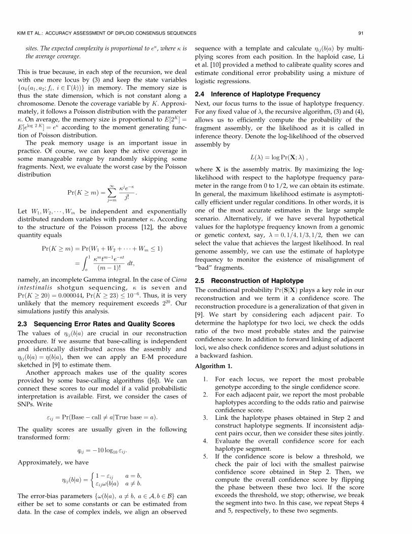
3.5 MLE of Haplotype Frequency

A theoretical assessment of the estimation is hard to establish

due to the complicated data structure. To study its statistical

performance, once again we used the simulation explained

earlier except that the scaffold size was 120K bp. The left side

of Fig. 8 shows the histogram of MLE when the true

frequency is one-quarter. It is approximately a normal

distribution. The right side of Fig. 8 shows the histogram of

MLE when the true frequency is one-half. The averages and

standard deviations of the estimates are shown in Table 4.

The larger the scaffold size, the more accurate the MLE.

The estimation of haplotype frequency can be applied to

the detection of duplications in shotgun sequencing. Fig. 9

shows the log-likelihood as a function of the haplotype

frequency, respectively, for the heterozygous and homo-

zygous cases. The scaffold size was 120k bp. As expected,

the likelihoods were maximized, respectively, at around

one-half and zero. In comparison, the change of coverage

has been used as an indication of duplication [3]. In

practice, we estimate haplotype frequency for each contig

and a significant change in value may indicate that an

abnormality, such as misalignment, has occurred.

3.6 Composition Probabilities

Other than sequencing error rates and haplotype frequency,

the parameters in our model also include the compositional

probabilities. Churchill and Waterman [4] derived an E-M

procedure to estimate the compositional probabilities,

sequencing error rates from the assembly for the one-

chromosome problem. In principle, similar ideas apply to

our case. If we assume independence of composition

between two haplotypes, then we have a more parsimo-

nious representation: �ða; bÞ ¼ �ðaÞ�ðbÞ. With the informa-

tion of S, the estimates of composition probabilities are

simply frequencies. The iterative E-M algorithm is based on

estimation of S. We note that the conditional probabilities

PrðSjXÞ are no longer independent among polymorphic

sites and we have to estimate them jointly. Computation-

ally, this is a challenging problem due to the large size of

the space S. The following strategy is easy to implement:

. Reconstruct the most likely haplotype under the

current parameter values.


TABLE 3Error Patterns

The polymorphism rate is 1.2 percent.

Fig. 6. Examples of accuracy assessment. The haplotype segments with positions, sizes, and confidence scores are produced by our program.

Fig. 7. Observed error rates versus nominal scores calculated by (4)and (3).

. Update the frequency of each of the positive

nucleotide bases.

3.7 Code

We have coded the algorithms presented in the paper in C

on the Linux platform and have tested them on various

simulation examples. We will be happy to send our code to

readers at their request.

APPENDIX

Proof of Theorem 1. Because the derivation is quite lengthy,we include some explanatory remarks after each step.Without loss of clarity, we use the same letter in differentsubscripts in the same line. The scope of each subscript isrestricted by its domain. These domains are separated bysemicolons or can be identified from the context.According to the definition of �k, only the fragments in�ðkÞ are relevant. Therefore, we have

�kþ1ða1; a2; fi; i 2 �ðkþ 1ÞÞ¼ PrðXij ¼ xij; j ¼ 1; . . . ; k; i 2 �ðkþ 1Þ;Skþ1;1 ¼ a1; Skþ1;2 ¼ a2;Fi ¼ fi; i 2 �ðkþ 1ÞÞðnext sum over cases of �1ðkþ 1Þ and �2ðkþ 1ÞÞsince �ðkþ 1Þ ¼ �3ðkþ 1Þ [ �4ðkþ 1ÞÞ¼Xb1;b2

Xfi¼1;2; i2�1ðkþ1Þ[�2ðkþ1Þ

fPrðXij ¼ xij; j ¼ 1; . . . ; kþ 1;

i 2 �ðkþ 1Þ;Sk;1 ¼ b1; Sk;2 ¼ b2;

Skþ1;1 ¼ a1; Skþ1;2 ¼ a2;Fi ¼ fi; i 2 �ðkþ 1ÞÞg

ðnext apply the Markov structureÞ¼Xb1;b2

Xfi¼1;2; i2�1ðkþ1Þ[�2ðkþ1Þ

fPrðXi;kþ1 ¼ xi;kþ1; i 2 �ðkþ 1ÞjSkþ1;1 ¼ a1; Skþ1;2 ¼ a2;

Fi ¼ fi; i 2 �ðkþ 1ÞÞPrðXij ¼ xij; j ¼ 1; . . . ; k; i 2 �ðkÞ;Sk;1 ¼ b1; Sk;2 ¼ b2;

Skþ1;1 ¼ a1; Skþ1;2 ¼ a2;Fi ¼ fi; i 2 �ðkþ 1ÞÞgðnotice that �ðkÞ ¼ �2ðkþ 1Þ

[�4ðkþ 1ÞÞ

¼Xb1;b2

Xfi¼1;2 i2�1ðkþ1Þ

Xfi¼1;2; i2�2ðkþ1Þ

fPrðXi;kþ1 ¼ xi;kþ1; i 2 �ðkþ 1ÞjSkþ1;1 ¼ a1; Skþ1;2 ¼ a2;

Fi ¼ fi; i 2 �ðkþ 1ÞÞPrðXij ¼ xij; j ¼ 1; . . . ; k; i 2 �ðkÞ;Sk;1 ¼ b1; Sk;2 ¼ b2;

Skþ1;1 ¼ a1; Skþ1;2 ¼ a2;Fi ¼ fi; i 2 �ðkÞ;Fi ¼ fi; i 2 �1ðkþ 1Þ;Fi ¼ fi; i 2 �3ðkþ 1ÞÞg

ðnext factorize some quantities by independence of fragments

and base compositionsÞ¼Xb1;b2

Xfi i2�1ðkþ1Þ

Xfi; i2�2ðkþ1Þ(� Y

i2�ðkþ1ÞPrðXi;kþ1 ¼ xi;kþ1jSkþ1;fi ¼ afiÞ

�

PrðXij ¼ xij; i 2 �ðkÞ; j ¼ 1; . . . ; k;Sk;1 ¼ b1; Sk;2 ¼ b2;

Fi ¼ fi; i 2 �ðkÞÞPrðSkþ1;1 ¼ a1; Skþ1;2 ¼ a2Þ

PrðFi ¼ fi; i 2 �1ðkþ 1ÞÞPrðFi ¼ fi; i 2 �3ðkþ 1ÞÞ)

ðnotice that �ðkþ 1Þ ¼ �1ðkþ 1Þ[

�2ðkþ 1Þ[

�3ðkþ 1Þ[�4ðkþ 1Þ and move common terms out of summationÞ


Fig. 8. Histograms of MLE estimates. Fragments were generated from scaffolds of size 120K bp. Left: The true haplotype frequency is one-quarter.

Right: The true haplotype frequency is one-half.

TABLE 4Statistics of the Maximum Likelihood Estimates of

Haplotype Frequency

¼ PrðSkþ1;1 ¼ a1; Skþ1;2 ¼ a2ÞPrðFi ¼ fi; i 2 �3ðkþ 1ÞÞ

Yi2�3ðkþ1Þ[�4ðkþ1Þ

PrðXi;kþ1 ¼ xi;kþ1jSkþ1;Fi ¼ afiÞ

24

35

Xb1;b2

Xfi; i2�2ðkþ1Þ

(�kðb1; b2; fi; i 2 �ðkÞÞ

Yi2�2ðkþ1Þ

PrðXi;kþ1 ¼ xi;kþ1jSkþ1;Fi ¼ afiÞ

24

35

Xfi; i2�1ðkþ1Þ

PrðFi ¼ fi; i 2 �1ðkþ 1ÞÞ

24Y

i2�1ðkþ1ÞPrðXi;kþ1 ¼ xi;kþ1jSkþ1;Fi ¼ afiÞ

35)

ðThe last line isY

i2�1ðkþ1Þ½�1�ðxi;kþ1ja1Þ þ �2�ðxi;kþ1ja2Þ

24

35Þ

¼ PrðSkþ1;1 ¼ a1; Skþ1;2 ¼ a2ÞY2

h¼1

�


h

� �

Yi2�3ðkþ1Þ[�4ðkþ1Þ

�ðxi;kþ1jafiÞ

24

35

Xb1;b2

Xfi; i2�2ðkþ1Þ

(�kðb1; b2; fi; i 2 �ðkÞÞÞ

Yi2�2ðkþ1Þ

�ðxi;kþ1jafiÞ

24

35

Yi2�1ðkþ1Þ

½�1�ðxi;kþ1ja1Þ þ �2�ðxi;kþ1ja2Þ�

24

35)

ðmove the terms relating to �1ðkþ 1Þ out of summation

and rearrange summationsÞ

¼ PrðSkþ1;1 ¼ a1; Skþ1;2 ¼ a2ÞY2

h¼1

�


h

" #

Yj2�1ðkþ1Þ

½�1 �ðxj;kþ1ja1Þ þ �2 �ðxj;kþ1ja2Þ

24

35

Yj2�3ðkþ1Þ[�4ðkþ1Þ

�ðxj;kþ1jafjÞ

24

35

Xfj¼1;2; j2�2ðkþ1Þ

Yj2�2ðkþ1Þ

�ðxj;kþ1jafjÞ

24

35

8<:Xb1;b2

�kðb1; b2; fj; j 2 �ðkÞÞ):

ut

ACKNOWLEDGMENTS

This work was supported by the Center of Excellence in

Genome Science at the University of Southern California, US

National Institutes of Health (NIH) P50 HG002790 CEGS

grant. The real sequence data of Ciona intestinalis were

produced by the US Department of Energy Joint Genome

Institute, http://www.jgi.doe.gov/. Lei M. Li’s work is

partially supported by grant R01 GM75308-01 from the NIH.

REFERENCES

[1] M.D. Adams et al., “The Genome Sequence of DrosophilaMelanogaster,” Science, vol. 287, pp. 2185-2195, 2000.

[2] S. Aparicio et al., “Whole-Genome Shotgun Assembly andAnalysis of the Genome of Fugu Rubripes,” Science, vol. 297,pp. 1301-1310, 2002.

[3] J.A. Bailey et al., “Recent Segmental Duplications in the HumanGenome,” Science, vol. 297, pp. 1003-1007, 2002.

[4] G.A. Churchill and M.S. Waterman, “The Accuracy of DNASequences: Estimating Sequence Quality,” Genomics, vol. 14,pp. 89-98, 1992.


Fig. 9. The log-likelihood curve—logarithm of probability of observations as a function of haplotype frequency. The scaffold size is 120K bp. Left: The

true haplotype frequency is one-half. Right: The true haplotype frequency is one—homozygous case.

[5] P. Dehal et al., “The Draft Genome of Ciona Intestinalis: Insightsinto Chordate and Vertebrate Origins,” Science, vol. 298, pp. 2157-2167, 2002.

[6] B. Ewing and P. Green, “Base-Calling of Automated SequencerTraces Using phred. 2. Error Probabilities,” Genome Research, vol. 8,pp. 186-194, 1998.

[7] G. Lancia, V. Bafna, S. Istrail, R. Lippert, and R. Schwartz, “SNPsProblems, Complexity, and Algorithms,” Proc. European Symp.Algorithms, pp. 182-193, 2001.

[8] E.S. Lander and M.S. Waterman, “Genomic Mapping by Finger-printing Random Clones,” Genomics, vol. 2, pp. 231-239, 1998.

[9] L.M. Li, J.H. Kim, and M.S. Waterman, “Haplotype Reconstruc-tion from SNP Alignment,” J. Computational Biology, vol. 11,pp. 505-516, 2004.

[10] M. Li, M. Nordborg, and L.M. Li, “Adjusted Quality Scores fromAlignment and Improve Sequencing Accuracy,” Nucleic AcidResearch, vol. 32, pp. 5183-5191, 2004.

[11] R. Lippert, R. Schwartz, G. Lancia, and S. Istrail, “AlgorithmicStrategies for the SNP Haplotype Assembly Problem,” Briefings inBioinformatics, vol. 3, pp. 1-9, 2002.

[12] S.M. Ross, Introduction to Probability Models, fourth ed. AcademicPress, 1989.

[13] J.C. Venter et al., “The Sequence of the Human Genome,” Science,vol. 291, pp. 1304-1351, 2001.

Jong Hyun Kim received the bachelor’s degreefrom Yonsei University in 2001. He is a PhDcandidate in the Department of ComputerScience at the University of Southen California.He is interested in applying computationalmethods to the fields of genomics and systemsbiology.

Michael S. Waterman is a professor of biologi-cal sciences, mathematics, and computerscience at the University of Southern California.He is a founding editor of the Journal ofComputational Biology and is coauthor of thetexts Computational Genome Analysis: An In-troduction and Introduction to ComputationalBiology: Maps, Sequences and Genomes.

Lei M. Li received the BS degree in mathe-matics and the MS degree in statistics in 1988and 1991, respectively, from Peking University,China, and the PhD degree in statistics in 1998from the University of California at Berkeley. Heis currently an associate professor of computa-tional biology and mathematics at the Universityof Southern California. His research interestsinclude computational biology and bioinfor-matics, statistical modeling, and computation.

. For more information on this or any other computing topic,please visit our Digital Library at www.computer.org/publications/dlib.


88 IEEE/ACM TRANSACTIONS ON COMPUTATIONAL … · Accuracy Assessment of Diploid Consensus Sequences...

Documents

Transcript of 88 IEEE/ACM TRANSACTIONS ON COMPUTATIONAL … · Accuracy Assessment of Diploid Consensus Sequences...