84 IEEE/ACM TRANSACTIONS ON NETWORKING, VOL. …metro.cs.ucla.edu/papers/ton12-dac.pdf · errors...

84 IEEE/ACM TRANSACTIONS ON NETWORKING, VOL. 20, NO. 1, FEBRUARY 2012

DAC: Generic and Automatic Address Configurationfor Data Center Networks

Kai Chen, Chuanxiong Guo, Haitao Wu, Member, IEEE, Jing Yuan, Zhenqian Feng, Yan Chen,Songwu Lu, Senior Member, IEEE, and Wenfei Wu

Abstract—Data center networks encode locality and topology in-formation into their server and switch addresses for performanceand routing purposes. For this reason, the traditional addressconfiguration protocols such as DHCP require a huge amount ofmanual input, leaving them error-prone. In this paper, we presentDAC, a generic and automatic Data center Address Configurationsystem. With an automatically generated blueprint that definesthe connections of servers and switches labeled by logical IDs,e.g., IP addresses, DAC first learns the physical topology labeledby device IDs, e.g., MAC addresses. Then, at the core of DACis its device-to-logical ID mapping and malfunction detection.DAC makes an innovation in abstracting the device-to-logical IDmapping to the graph isomorphism problem and solves it withlow time complexity by leveraging the attributes of data centernetwork topologies. Its malfunction detection scheme detectserrors such as device and link failures and miswirings, includingthe most difficult case where miswirings do not cause any nodedegree change. We have evaluated DAC via simulation, implemen-tation, and experiments. Our simulation results show that DACcan accurately find all the hardest-to-detect malfunctions andcan autoconfigure a large data center with 3.8 million devices in46 s. In our implementation, we successfully autoconfigure a small64-server BCube network within 300 ms and show that DAC is aviable solution for data center autoconfiguration.

Index Terms—Address configuration, data center networks(DCNs), graph isomorphism.

I. INTRODUCTION

A. Motivation

M EGA data centers [1] are being built around the worldto provide various cloud computing services such as

Web search, online social networking, online office, and IT

Manuscript received October 11, 2010; revised March 03, 2011; acceptedMay 06, 2011; approved by IEEE/ACM TRANSACTIONS ON NETWORKING Ed-itor S. Kalyanaraman. Date of publication June 02, 2011; date of current versionFebruary 15, 2012. This work was performed when K. Chen, Z. Feng, and W.Wu were interns at Microsoft Research Asia.K. Chen is with Northwestern University, Evanston, IL 60208 USA (e-mail:

[email protected]).C. Guo and H. Wu are with Microsoft Research Asia, Beijing 100190, China

(e-mail: [email protected]; [email protected]).J. Yuan is with Tsinghua University, Beijing 100084, China (e-mail: yuan-

[email protected]).Z. Feng is with the National University of Defense Technology, Changsha

410073, China (e-mail: [email protected]).Y. Chen is with Northwestern University, Evanston, IL 60208 USA (e-mail:

[email protected]).S. Lu is with the University of California, Los Angeles, CA 90095 USA

(e-mail: [email protected]).W. Wu is with the University of Wisconsin–Madison, Madison, WI 53706

USA (e-mail: [email protected]).Color versions of one or more of the figures in this paper are available online

at http://ieeexplore.ieee.org.Digital Object Identifier 10.1109/TNET.2011.2157520

infrastructure outsourcing for both individual users and organi-zations. To take advantage of economies of scale, it is commonfor a data center to contain tens or even hundreds of thousandsof servers. The current choice for building data centers is usingcommodity servers and Ethernet switches for hardware and thestandard TCP/IP protocol suite for interserver communication.This choice provides the best performance to price tradeoff [2].All the servers are connected via network switches to form alarge distributed system.Before the servers and switches can provide any useful ser-

vices, however, they must be correctly configured. For existingdata centers using the TCP/IP protocol, the configuration in-cludes assigning an IP address to every server. For layer-2 Eth-ernet, we can use DHCP [3] for dynamic IP address configura-tion. However, servers in a data center need more than one IPaddress in certain address ranges. This is because, for perfor-mance and fault tolerance reasons, servers need to know the lo-cality of other servers. For example, in a distributed file system[4], a chunk of data is replicated several times, typically three,to increase reliability. It is better to put the second replica on aserver in the same rack as the original, and the third replica on aserver at another rack. The current practice is to embed localityinformation into IP addresses. The address locality can also beused to increase performance. For example, instead of fetchinga piece of data from a distant server, we can retrieve the samepiece of data from a closer one. This kind of locality-based op-timization is widely used in data center applications [4], [5].The newly proposed data center network (DCN) struc-

tures [6]–[9] go one step further by encoding their topologyinformation into their logical IDs. These logical IDs can takethe form of IP address (e.g., in VL2 [9]), MAC address (e.g.,in Portland [8]), or even newly invented IDs (e.g., in DCell [6]and BCube [7]). These structures then leverage the topologicalinformation embedded in the logical IDs for scalable and effi-cient routing. For example, Portland switches choose a routingpath by exploiting the location information of destinationPseudo-MAC (PMAC). BCube servers build a source routingpath by modifying one digit at one step based on source anddestination BCube IDs.For all the cases above, we need to configure the logical IDs,

which may be IP or MAC addresses or BCube or DCell IDs,for all the servers and switches. Meanwhile, in the physicaltopology, all the devices are identified by their unique deviceIDs, such as MAC addresses. A naïve way is to build a static de-vice-to-logical ID mapping table at the DHCP server. Buildingsuch a table is mainly a manual effort that does not work forthe following two reasons. First of all, the scale of data centeris huge. It is not uncommon that a mega data center can havehundreds of thousands of servers [1]. Second, manual config-uration is error-prone. A recent survey from 100 data center

1063-6692/$26.00 © 2011 IEEE

CHEN et al.: DAC: GENERIC AND AUTOMATIC ADDRESS CONFIGURATION FOR DATA CENTER NETWORKS 85

professionals [10] suggested that 57% of the data center out-ages are caused by human errors. Two more surveys [11], [12]showed 50%–80% of network downtime is due to human con-figuration errors. In short, “the vast majority of failures in datacenters are caused, triggered or exacerbated by human errors”[13].

B. Challenges and Contributions

Automatic address configuration is therefore highly desirablefor data center networks. We envision that a good autoconfigu-ration system will have the following features, which also posechallenges for building such a system.• Generality: The system needs to be applicable to variousnetwork topologies and addressing schemes.

• Efficiency and scalability: The system should assign a log-ical ID to a device quickly and be scalable to a large numberof devices.

• Malfunction and error handling: The system must be ableto handle various malfunctions such as broken NICs andwires and human errors such as miswirings.

• Minimal human intervention: The system should requireminimal manual effort to reduce human errors.

To the best of our knowledge, there are very few existingsolutions, and none of them can meet all the requirementsabove. In this paper, we address these problems by proposingDAC—a generic and automatic Data center Address Configu-ration system for the existing and future data center networks.To make our solution generic, we assume that we only have ablueprint of the to-be-configured data center network, whichdefines how the servers and switches are connected and labelseach device with a logical ID. The blueprint can be automat-ically generated because all the existing data center networkstructures are quite regular and can be described either recur-sively or iteratively (see [6]–[9] for examples).Through a physical network topology learning procedure that

we will describe in Section V, DAC first automatically learnsand stores the physical topology of the data center network intoan autoconfiguration manager. Then, we make the followingtwo key contributions when designing DAC.First of all, we solve the core problem of autoconfiguration:

how to map the device IDs in the physical topology to the log-ical IDs in the blueprint while preserving the topological re-lationship of these devices. DAC makes an innovation in ab-stracting the device-to-logical ID mapping to the graph isomor-phism (GI) problem [14] in graph theory. Existing GI solutionsare too slow for some large-scale data center networks. Based onthe attributes of data center network topologies, such as sparsityand symmetry (or asymmetry), we apply graph theory knowl-edge to design an improved algorithm that significantly speedsup the mapping. Specifically, we use three speedup techniques:candidate selection via SPLD, candidate pruning via orbit, andselective splitting. The first technique is our own. The last twowe selected from previous works [15] and [16], respectively,after finding that they are quite effective for data center graphs.Second, despite that the malfunction detection problem is

NP-complete and APX-hard,1 we design a practical scheme thatsubtly exploits the degree regularity in all data center structuresto detect the malfunctions causing device degree change. For

1A problem is APX-hard if there is no polynomial-time approximationscheme.

the hardest one with no degree change, we propose a schemeto compare the blueprint graph and the physical topology graphfrom multiple anchor points and correlate malfunctions via ma-jority voting. Evaluation shows that our solution is fast and isable to detect all the hardest-to-detect malfunctions.We have studied our DAC design via extensive experiments

and simulations. The experimental results show that the timeof our device-to-logical ID mapping scales in proportion to thetotal number of devices in the networks. Furthermore, our sim-ulation results show that DAC can autoconfigure a large datacenter with 3.8 million devices in 46 s. We have also devel-oped and implemented DAC as an application on a 64-servertest bed, where the 64 servers and 16 mini-switches form atwo-level BCube [7] network. Our autoconfiguration protocolsautomatically and accurately assign BCube logical IDs to these64 servers within 300 ms.Roadmap: The rest of the paper is organized as follows.

Section II presents the system overview. Section III introducesthe device-to-logical ID mapping. Section IV discusses howDAC deals with malfunctions. Sections V and VI evaluate DACvia experiments, simulations, and implementations. Section VIIdiscusses the related work. Section VIII concludes the paper.

II. SYSTEM OVERVIEW

One important characteristic shared by all data centers is thata given data center is owned and operated by a single organi-zation. DAC takes advantage of this property to employ a cen-tralized autoconfiguration manager, which we call DAC man-ager throughout this paper. DAC manager deals with all theaddress configuration intelligences such as physical topologycollection, device-to-logical ID mapping, logical ID dissemina-tion, and malfunction detection. In our design, DAC managercan simply be a server in the physical topology or can run on aseparate control network.Our centralized design is also inspired by the success of sev-

eral recent large-scale infrastructure deployments. For instance,the data processing system MapReduce [5] and the modernstorage GFS [4] employ a central master at the scale of tens ofthousands of devices. More recently, Portland [8] leverages afabric manager to realize a scalable and efficient layer-2 datacenter network fabric.As stated in our first design goal, DAC should be a generic

solution for various topologies and addressing schemes. Toachieve this, DAC cannot assume any specific form of structureor addressing scheme in its design. Considering this, DAC onlyuses the following two graphs as its input.1) Blueprint: Data centers have well-defined structures.

Prior to deploying a real data center, a blueprint [Fig. 1(a)]should be designed to guide the construction of the data center.To make our solution generic, we only require the blueprint toprovide the following minimal information.• Interconnections between devices: It should define the in-terconnections between devices. Note that though it is pos-sible for a blueprint to label port numbers and define howthe ports of neighboring devices are connected, DAC doesnot depend on such information. DAC only requires theneighbor information of the devices, contained in any con-nected graph.


Fig. 1. Example of blueprint and physical topology constructed by followingthe interconnections in blueprint. (a) Blueprint: Each node has a logical ID.(b) Physical network topology: Each device has a device ID.

Fig. 2. DAC system framework with four modules.

• Logical ID for each device: It should specify a logical IDfor each device.2 The encoding of these logical IDs con-veys the topological information of the network structure.These logical IDs are vital for server communication androuting protocols.

Since data center networks are quite regular and can be de-scribed iteratively or recursively, we can automatically generatethe blueprint using software.2) Physical Network Topology: The physical topology

[Fig. 1(b)] is constructed by following the interconnectionsdefined in the blueprint. In this physical topology, we use theMAC address as a device ID to uniquely identify a device. Fora device with multiple MAC addresses, we use the lowest one.In the rest of the paper, we use to denote

the blueprint graph and to denote the physicaltopology graph. are the set of nodes (i.e., devices) withlogical/device IDs, respectively, and are the set of edges(i.e., links). Note that while the blueprint graph is known forany data center, the physical topology graph is not knownuntil the data center is built and information collected.The whole DAC system structure is illustrated in Fig. 2. The

two core components of DAC are device-to-logical ID mappingandmalfunction detection and handling. We also have a moduleto collect the physical topology and a module to disseminate thelogical IDs to individual devices after DACmanager finishes thedevice-to-logical IDmapping. In what follows, we overview thedesign of these modules.3) Physical Topology Collection: In order to perform logical

ID resolution, we need to know both blueprint and phys-ical topology . Since is not known readily, DAC requiresa communication channel over the physical network to collectthe physical topology information. To this end, we propose a

2While most data center structures, like BCube [7], DCell [6], Ficonn [17],and Portland [8], use device-based logical ID, there also exist structures, likeVL2 [9], that use port-based logical ID. For brevity, in this paper, DAC is in-troduced and evaluated as the device based case. It can handle the port-basedscenario by simply considering each port as a single device and treating a devicewith multiple ports as multiple logical devices.

Communication channel Building Protocol (CBP). The channelbuilt from CBP is a layered spanning tree, and the root is DACmanager with level 0, its children are level 1, so on and so forth.When the channel is built, the next step is to collect the phys-

ical topology . For this, we introduce a Physical topologyCollection Protocol (PCP). In PCP, the physical topology in-formation, i.e., the connection information between each node,is propagated bottom–up from the leaf devices to the root (i.e.,DAC manager) layer by layer. After is collected by DACmanager, we go to the device-to-logical ID mapping module.4) Device-to-Logical ID Mapping: After has been col-

lected, we come to device-to-logical IDmapping, which is a keycomponent of DAC. As introduced in Section I, the challengeis how to have the mapping reflect the topological relationshipof these devices. To this end, we devise , a fast one-to-onemapping engine, to realize this functionality. We elaborate thisfully in Section III.5) Logical ID Dissemination: When logical IDs for all the

devices have been resolved, i.e., the device-to-logical ID map-ping table is achieved, we need to disseminate this informationto the whole network. To this end, we introduce a Logical IDDissemination Protocol (LDP). In contrast to PCP, in LDP themapping table is delivered top–down from DACmanager to theleaf devices, layer by layer. Upon receipt of such information,a device can easily index its logical ID according to its deviceID. A more detailed explanation of LDP together with CBP andPCP is introduced in Section V.6) Malfunction Detection and Handling: DAC needs to au-

tomatically detect malfunctions and pinpoint their locations. Forthis, we introduce amalfunction detection and handlingmodule.In DAC, this module interacts tightly with the device-to-logicalID mapping module because the former one is only triggeredby the latter. If there exist malfunctions in , our enginequickly perceives this by noticing that the physical topologygraph mismatches with the blueprint graph . Then, themalfunction detection module is immediately invoked to detectthose malfunctioning devices and report them to network ad-ministrators. We describe this module in Section IV.

III. DEVICE-TO-LOGICAL ID MAPPING

In this section, we formally introduce how DAC performs thedevice-to-logical ID mapping. We first formulate the mappingusing graph theory. Then, we solve the problem via optimiza-tions designed for data center structures. Lastly, we discuss howto do the mapping for data center expansion.

A. Problem Formulation and Solution Overview

As introduced, the challenge here is to do the device-to-log-ical mapping such that this mapping reflects the topological re-lationship of these devices. Considering we have the blueprintgraph and the physical topology graph

, to meet the above requirement, we formulate the map-ping problem as finding a one-to-one mapping between nodesin and while preserving the adjacencies in and .Interestingly, this is actually a variant of the classical graph iso-morphism (GI) problem [14].Definition 1: Two graphs and

are isomorphic, denoted by , if there is a bijection


Fig. 3. mapping engine.

such that if and only if, for all , . Such a bijection is called a graph iso-

morphism between and .To the best of our knowledge, we are the first to introduce the

GI model to data center networks, thus solving the address auto-configuration problem. After the problem formulation, the nextstep is to solve the GI problem. In the past 20 years, many re-search efforts have been made to determine whether the generalGI problem is in P or NP [14]. When the maximum node degreeis bounded, polynomial algorithm with time complexityis known [18], where is the number of nodes and is the max-imum node degree.However, is too slow for our problem since data cen-

ters can have millions of devices [6] and the maximal node de-gree can be more than 100 [9]. To this end, we devise , afast one-to-one mapping engine. As shown in Fig. 3, startswith a base algorithm (i.e., ) for generalgraphs, and upon that we propose an improved algorithm (i.e.,

) using three speedup techniques: candidate se-lection via SPLD, candidate filtering via orbit, and selectivesplitting, which are specially tailored for the attributes of datacenter structures and our real address autoconfiguration applica-tion. In the following, we first introduce some preliminaries to-gether with the base algorithm, and then introduce the improvedalgorithm.

B. Base Algorithm

1) Preliminaries: Given a graph , a partitionof a vertex set , e.g., , is a set ofdisjoint nonempty subsets of whose union is . We call eachsubset a cell. In , the basic operations onpartitions or cells are “decompose” and “split.”• Decompose: Given a node , a cell , and a partitionwhere and , using to decompose meansto replace with and in partition , where isset minus meaning to remove node from .

• Split: Given two cells , , using to splitmeans doing the following. First, for each node ,we calculate a value as the number of con-nections between node and nodes in where is calledconnection function. Then, we divide into smaller cellsby grouping the nodes with the same value together to bea new cell. Moreover, we call the inducing cell andthe target cell. The target cell should be a non-singleton.

A partition is equitable if no cell can be split by any other cellin the partition. A partition is discrete if each cell of this par-tition is a singleton (i.e., single element). Suppose we use an

Fig. 4. Pseudocode of the generic algorithm for one-to-one mapping (i.e.,graph isomorphism). For clarity, the functions and

are explained in the context.

inducing cell pair to split target cell pair , respec-tively. are divided isomorphically by if for eachvalue , has the same number of nodes with-connection to as has to .Note that the cells in a partition have their orders. We use

parenthesis to represent a partition, and each cell is indexed byits order. For example, means a parti-tion with cells and the th cell is . In our mapping algo-rithm, decomposition/split operation always works on the cor-responding pair of cells (i.e., two cells with the same order) intwo partitions. Furthermore, during these operations, we placethe split cells back to the partitions in corresponding orders. Forexample, decomposing with , we replace with, and with , , and then place the split

cells back to the partitions such that and are in the sameorder and and are in the same order.In addition to the above terms, we further have two impor-

tant terms used in the improved algorithm, which are SPLD andorbit.• SPLD: SPLD is short for shortest path length distribution.The SPLD of a node is the distribution of distances be-tween this node and all other nodes in the graph.

• Orbit: An orbit is a subset of nodes in graph such thattwo nodes and are in the same orbit if there existsan automorphism3 of that maps to [19]. For ex-ample, in of Fig. 6, to are in the same orbit sincethere is an automorphism permutation of , which is

, that maps to .2) Base Algorithm: Fig. 4 is a base mapping algorithm for

general graphs we summarize from previous literature. It con-tains and , and it repeatedlydecomposes and refines (or splits) and until either theyboth are discrete, or it terminates in the middle finding thatand are not isomorphic.In each level of recursion, we first check if the current par-

titions and are discrete. If so, we return (line 2)and get a one-to-one mapping by mapping each singleton cellof to the corresponding singleton cell of . Otherwise, wedo .

3An automorphism of a graph is a graph isomorphism with itself, i.e., a map-ping from the vertices of the given graph back to vertices of such that theresulting graph is isomorphic with .


In , we first select a pair of corre-sponding non-singleton cells and , and then se-lect a pair of nodes and to decom-pose and , respectively (lines 4–6). Then, weget partitions and

. Immediately afterdecomposition, we do on and (line 7).In , we repeatedly try to use every newly born

pair of cells to split all other corresponding non-singleton pairsof cells. For each pair of cells that have been simultaneouslydivided, we check whether the two cells are divided isomorphi-cally or not. If not, then returns .Otherwise, if each time the pair of target cells are isomorphicallydivided, will continue until andare equitable and returns .If returns true, we go one step further

of recursion to work on new equitable partitions (line 8). Oth-erwise, it means that cannot be mapped to , and we try thenext candidate in (line 11). If all the candidates in failto be mapped to , we must backtrack (line 10). Such recur-sion continues until either both partitions become discrete, i.e.,a one-to-one mapping is found (line 2), or we backtrack to rootof the search tree, thus concluding that no one-to-one mappingexists (line 12).

C. Improved Algorithm

Compared to general graphs, network topologies of data cen-ters have the following attributes: 1) they are sparse; 2) theyare typically either highly symmetric like BCube [7] or highlyasymmetric like DCell [6]. In any case, for our address autocon-figuration problem, the blueprint graph is available in advance,which means we can do some precomputation.Based on these features, we apply graph theory to design an

improved algorithm with three speedup techniques: candidateselection via SPLD, candidate filtering via orbit, and selectivesplitting to speed up the device-to-logical ID mapping. Specif-ically, we introduce the first technique and borrow the last twofrom [15] and [16], respectively, based on their effectivenessfor graphs derived for data centers. We prove that adding thesespeedup techniques to the base algorithm maintains its cor-rectness [20]. Our experiments in Section VI-B indicate that weneed all these three speedup techniques to solve our problem,and any partial combination of them is slow for some structures.Fig. 5 is the improved algorithm built on the base algorithm. Inthe following, we explain the three speedup techniques empha-sizing the reasons why they are suitable for data center graphs.1) Candidate Selection via SPLD: We observe that nodes in

data centers have different roles such as switches and servers,and switches in some data centers like FatTree can be further di-vided into ToR, aggregation, and core. Hence, from this point ofview, SPLD can be helpful by itself to distinguish nodes of dif-ferent roles. Furthermore, SPLD can provide even significantimprovement for structures like DCell, which are very asym-metric. This is because the SPLDs of different nodes in DCellare very different. To take advantage of this property, we pro-pose using SPLD as a more sophisticated signature to selectmapping candidates. That is, when we try to select a node in

Fig. 5. Pseudocode of the improved algorithm for data center graphs. Forclarity, is explained in the context.

as a candidate to be mapped to a node in , we only se-lect the from these nodes that have the same SPLD as . Thisis effective because two nodes with different SPLDs cannot bemapped to each other. However, computing SPLDs for all nodesin a large graph requires time. Fortunately, this can be computedearlier on the blueprint.In our improved algorithm, we precompute the SPLDs for

all nodes of beforehand. In lines 6 and 7, we improve thebase algorithm in this way: If we find the number of candidates(i.e., nodes in ) for a node, say in , to be mapped to islarger than a threshold (i.e., ) and the numberof different SPLDs of them is larger than a threshold (i.e.,

), we compute the SPLD for and onlyselect candidates in having the same SPLD. Thresholdsand are tunable. Note that using this technique is a tradeoff:Althoughwe can do precomputation on offline, applying thisoptimization means that we should compute online,which also consumes time. In all our experiments later, we applythis technique on all the structures only once at the first roundof mapping.2) Candidate Filtering via Orbit: It is indicated in [15] that

for and , if cannot be mapped to , all nodes inthe same orbit as cannot be mapped to either. We find thistheory is naturally suited for solving the GI problem on datacenters. First, some structures such as BCube are highly sym-metric, and there should be many symmetric nodes within thesestructures that are in the same orbit. Second, the blueprint graphis available much earlier than the real address autoconfigurationstage, and we can easily precompute the orbits in the blueprintbeforehand using preexisting tools such as [16], [21].In Fig. 4, the base algorithm tries to map to every node in

iteratively if the current mapping fails, which is not effective es-pecially for highly symmetric data center structures. Observingthis, in the improved algorithm, we precompute all the orbits ofbeforehand. Then, as shown in lines 16–18, we improve the

base algorithm: If we find a certain node cannot be mappedto , we skip all the attempts that try to map to any other node


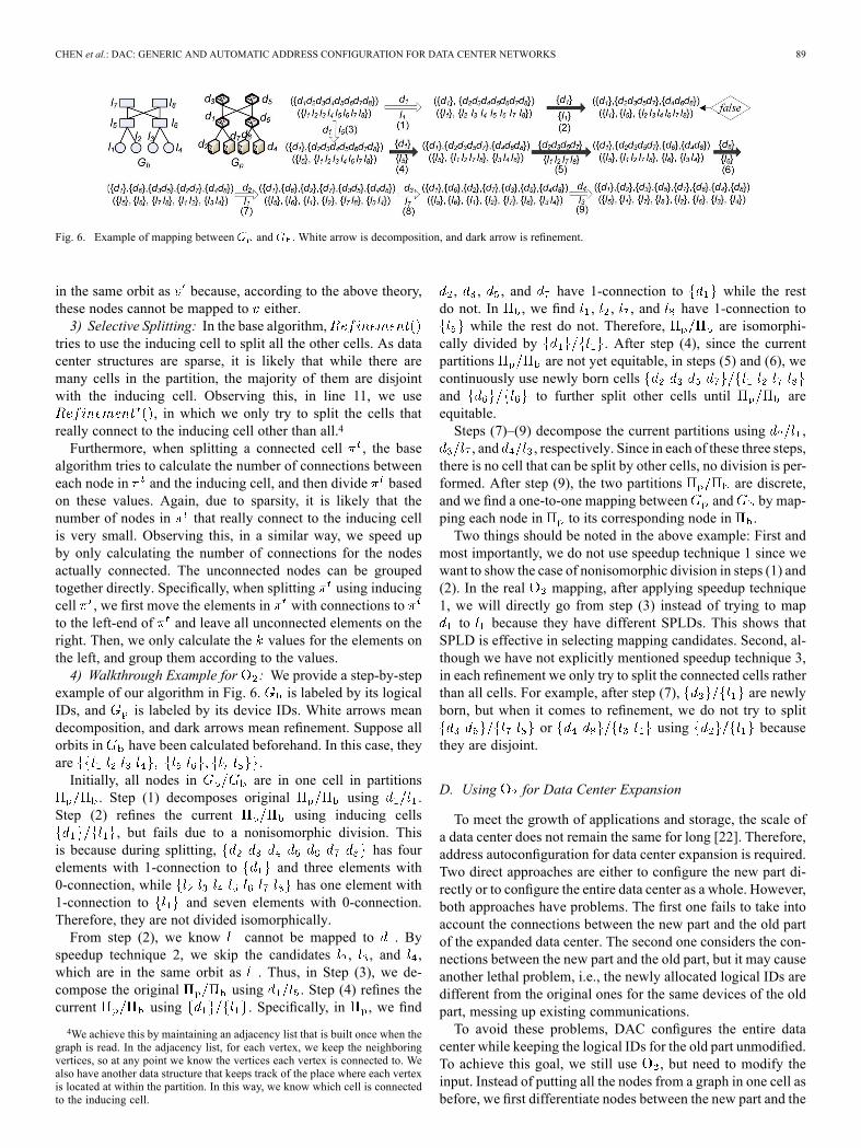
Fig. 6. Example of mapping between and . White arrow is decomposition, and dark arrow is refinement.

in the same orbit as because, according to the above theory,these nodes cannot be mapped to either.3) Selective Splitting: In the base algorithm,

tries to use the inducing cell to split all the other cells. As datacenter structures are sparse, it is likely that while there aremany cells in the partition, the majority of them are disjointwith the inducing cell. Observing this, in line 11, we use

, in which we only try to split the cells thatreally connect to the inducing cell other than all.4

Furthermore, when splitting a connected cell , the basealgorithm tries to calculate the number of connections betweeneach node in and the inducing cell, and then divide basedon these values. Again, due to sparsity, it is likely that thenumber of nodes in that really connect to the inducing cellis very small. Observing this, in a similar way, we speed upby only calculating the number of connections for the nodesactually connected. The unconnected nodes can be groupedtogether directly. Specifically, when splitting using inducingcell , we first move the elements in with connections toto the left-end of and leave all unconnected elements on theright. Then, we only calculate the values for the elements onthe left, and group them according to the values.4) Walkthrough Example for : We provide a step-by-step

example of our algorithm in Fig. 6. is labeled by its logicalIDs, and is labeled by its device IDs. White arrows meandecomposition, and dark arrows mean refinement. Suppose allorbits in have been calculated beforehand. In this case, theyare .Initially, all nodes in are in one cell in partitions

. Step (1) decomposes original using .Step (2) refines the current using inducing cells

, but fails due to a nonisomorphic division. Thisis because during splitting, has fourelements with 1-connection to and three elements with0-connection, while has one element with1-connection to and seven elements with 0-connection.Therefore, they are not divided isomorphically.From step (2), we know cannot be mapped to . By

speedup technique 2, we skip the candidates , , and ,which are in the same orbit as . Thus, in Step (3), we de-compose the original using . Step (4) refines thecurrent using . Specifically, in , we find

4We achieve this by maintaining an adjacency list that is built once when thegraph is read. In the adjacency list, for each vertex, we keep the neighboringvertices, so at any point we know the vertices each vertex is connected to. Wealso have another data structure that keeps track of the place where each vertexis located at within the partition. In this way, we know which cell is connectedto the inducing cell.

, , , and have 1-connection to while the restdo not. In , we find , , , and have 1-connection to

while the rest do not. Therefore, are isomorphi-cally divided by . After step (4), since the currentpartitions are not yet equitable, in steps (5) and (6), wecontinuously use newly born cellsand to further split other cells until areequitable.Steps (7)–(9) decompose the current partitions using ,, and , respectively. Since in each of these three steps,

there is no cell that can be split by other cells, no division is per-formed. After step (9), the two partitions are discrete,and we find a one-to-one mapping between and by map-ping each node in to its corresponding node in .Two things should be noted in the above example: First and

most importantly, we do not use speedup technique 1 since wewant to show the case of nonisomorphic division in steps (1) and(2). In the real mapping, after applying speedup technique1, we will directly go from step (3) instead of trying to mapto because they have different SPLDs. This shows that

SPLD is effective in selecting mapping candidates. Second, al-though we have not explicitly mentioned speedup technique 3,in each refinement we only try to split the connected cells ratherthan all cells. For example, after step (7), are newlyborn, but when it comes to refinement, we do not try to split

or using becausethey are disjoint.

D. Using for Data Center Expansion

To meet the growth of applications and storage, the scale ofa data center does not remain the same for long [22]. Therefore,address autoconfiguration for data center expansion is required.Two direct approaches are either to configure the new part di-rectly or to configure the entire data center as a whole. However,both approaches have problems. The first one fails to take intoaccount the connections between the new part and the old partof the expanded data center. The second one considers the con-nections between the new part and the old part, but it may causeanother lethal problem, i.e., the newly allocated logical IDs aredifferent from the original ones for the same devices of the oldpart, messing up existing communications.To avoid these problems, DAC configures the entire data

center while keeping the logical IDs for the old part unmodified.To achieve this goal, we still use , but need to modify theinput. Instead of putting all the nodes from a graph in one cell asbefore, we first differentiate nodes between the new part and the


old part in and . Since we already have the device-to-log-ical ID mapping for the old part, say for , weexplicitly express such one-to-one mapping in the partitions.In other words, we have and

, and all the nodes for the new partof are in , respectively. Then, we refineuntil they both are equitable. At last, we enter mappingwith the equitable partitions. In this way, we can produce adevice-to-logical ID mapping table for the new part of datacenter while keeping the logical IDs for devices of the old partunmodified.

IV. MALFUNCTION DETECTION AND HANDLING

As introduced before, the malfunction detection moduleis triggered when returns . This “false” indicatesthe physical topology is not the same as the blueprint. In thissection, we describe how DAC handles malfunctions.

A. Malfunction Overview

Malfunctions can be caused by hardware and software fail-ures or simply human configuration errors. For example, bad ormismatched network cards and cables are common, and mis-wired or improperly connected cables are nearly inevitable.We consider and categorize three malfunction types in data

centers: node, link, and miswiring. The first type occurs whena given server or switch breaks down from hardware or soft-ware reasons, causing it to be completely unreachable and dis-connected from the network. The second one occurs when thecable or network card is broken or not properly plugged in sothat the connectivity between devices on that link is lost. Thethird one occurs when wired cables are different from those inthe blueprint. These malfunctions may introduce severe prob-lems and downgrade the performance.Note that from the physical topology, it is unlikely to clearly

distinguish some failure types, e.g., a crashed server versuscompletely malfunctioning interface cards on that server. Ourgoal is to detect and further locate all malfunction-relateddevices and report the device information to network admin-istrators, rather than identifying the malfunction type. Webelieve our malfunction handling not only solves this issue forautoconfiguration, but also reduces the deployment/mainte-nance costs for real-world large data center deployment.

B. Problem Complexity and Challenge

The problem of malfunction detection can be formally de-scribed as follows. Given and , the problem to locateall the malfunctioning parts in the graph is equivalentto obtaining the maximum common subgraph (MCS)of and . Thus, we compare to to find thedifferences, which are the malfunctioning parts. All the devices(i.e., servers or switches) related to these parts, which we callmalfunctioning devices, can be detected. However, it is proventhat the MCS problem is NP-complete [23] and APX-hard [24].That is, there is no efficient algorithm, especially for largegraphs such as those of data center network topologies. There-fore, we resort to designing our own algorithms based on theparticular properties of data center structures and our real-world

TABLE IDEGREE PATTERNS IN BCUBE, FATTREE, VL2, AND DCELL STRUCTURES.

, , , ARE THE PARAMETERS TO DEFINE THESE NETWORKS.THEY ARE FIXED FOR A GIVEN STRUCTURE

application scenario. There are two problems we need to ad-dress in Sections IV-C–IV-E: 1) detecting the malfunctioningdevices by identifying their device IDs; and 2) locating thephysical position of a malfunctioning device with its device IDautomatically.

C. Practical Malfunction Detection Methods

To achieve better performance and easier management,large-scale data centers are usually designed and constructedaccording to some patterns or rules. Such patterns or rulesimply two properties of the data center structures. 1) The nodesin the topologies typically have regular degrees. For example,we show the degree patterns for several well-known datacenter networks in Table I. 2) The graphs are sparse, so thatour can quickly determine if two graphs are isomorphic.These properties are important for us to detect malfunctionsin data centers. In DAC, the first property is used to detectmalfunctioning devices where there are node degree changes,and the second one serves as a tool in our malfunction detectionscheme for the case where no degree change occurs.1) Malfunction With Node Degree Change: For the afore-

mentioned three types of malfunctions, we discuss them one byone as follows. Our observation is that most of the cases maycause the change of degree on devices.• Node: If there is a malfunctioning node, the degrees of itsneighboring nodes are decreased by one, and thus it is pos-sible to identify the malfunction by checking its neighbornodes.

• Link: If there is a malfunctioning link, the degrees of as-sociated nodes are decreased by one, making it possible todetect.

• Miswiring: Miswirings are somewhat more complex thanthe other two errors. As shown in the left of Fig. 7, themiswiring causes its related nodes to increase or decreasetheir degrees and can be detected readily. On the contrary,in the right of Fig. 7, the miswirings of a pair of cablesoccur coincidentally so that the degree change caused byone miswired cable is glossed over by another, and thus nonode degree change happens. We discuss this hardest caseseparately in the following.

Note that for any malfunction caused by the links, i.e., linkfailure or miswirings, we report the associated nodes (i.e., mal-functioning devices) in our malfunction detection.2) Malfunction Without Node Degree Change: Though

in most cases the malfunctions cause detectable node degreechange [25], it is still possible to have miswirings with no nodedegree change. This case occurs after an administrator haschecked the network and the degree-changing malfunctions


Fig. 7. Miswirings with and without degree change.

Fig. 8. Pseudocode for malfunction detection.

have been fixed. The practical assumptions here are: 1) thenumber of nodes involved in such malfunctions is a consider-ably small amount over all the nodes; 2) and have thesame number of nodes and node degree patterns.Despite the miswirings, the vast majority part of and

are still the same. We leverage this fact to detect such mis-wirings. Our basic idea is that we first find some nodes that aresupposed to be symmetric between and , then use thosenodes as anchor points to check if the subgraphs deduced fromthem are isomorphic. Through this we derive the difference be-tween the two graphs and correlate the malfunctioning candi-dates derived from different anchor points to make a decision.Basically, our scheme has two parts: anchor point selection andmalfunction detection.To minimize the human intervention, the first challenge is

selecting anchor pairs between the blueprint graph and thephysical topology graph without human input. Our ideais again to leverage the SPLD. Considering that the numberof nodes involved in miswirings is small, it is likely that two“symmetric” nodes in two graphs will still have similar SPLDs.Based on this, we design our heuristics to select anchor pairpoints, which is in Fig. 8. In thealgorithm, is simply the Euclideandistance. Given that two node with similar SPLDs are notnecessarily a truly symmetric pair, our malfunction detectionscheme will take the potential false positives into account andhandle this issue via majority voting.Once the anchor node pairs have been selected, we com-

pare and from these anchor node pairs and correlatemalfunctions via majority voting. The algorithm for this is

in Fig. 8. Specifically, given, and definition of maximal subgraph

in line 5, for each anchor pair , we search themaximal isomorphic subgraph of graphs with hoplength from nodes respectively. The process to obtainsuch a subgraph is in line 7. We can use a binary search toaccelerate the searching procedure. If we find that and

are isomorphic while and are not,we assume some miswirings happened between -hop and

-hop away from , and the nodes in these two hops aresuspicious. In line 9, we increase a counter for each of thesenodes to represent this conclusion.After finishing the detection from all the anchor points, we

report a list to the administrator. The list contains node deviceIDs and counter values of each node, ranked in the descendingorder of the counter values. Essentially, the larger its countervalue, the more likely the device is miswired. Then, the admin-istrator will go through the list and rectify the miswirings. Thisprocess stops when he finds a node is not really miswired andignores the rest of nodes on the list.The accuracy of our scheme depends on the number of

anchor points we selected for detection versus the number ofmiswirings in the network. Our experiments suggest that, witha sufficient number of anchor points, our algorithm can alwaysfind all the malfunctions (i.e., put the miswired devices on topof the output list). According to the experimental results inSection VI-D, with at most 1.5% of nodes selected as anchorpoints, we can detect all miswirings on the evaluated structures.To be more reliable, we can always conservatively select alarger percentage of anchor points to start our detection, andmost likely we will detect all miswirings (i.e., have all ofthem on top of the list). Actually, this can be facilitated by theparallel computing because in our malfunction detection, thecalculations from different anchor points are independent ofeach other and thus can be performed in parallel.After fixing the miswirings, we will run to get the de-

vice-to-logical ID mapping again. Even in the case that not allthe miswirings are on the top of the list and we miss some,will perceive that quickly. Then, we will rerun our detection al-gorithm until all miswirings are detected and rectified, andcan get the correct device-to-logical ID mapping finally.

D. Device Locating

Given a detected malfunctioning device, the next practicalquestion is how to identify the location of the device given onlyits device ID (i.e., MAC). In fact, the device locating procedureis not necessarily achieved by an autoconfiguration algorithm,but also possibly by some human efforts. In this paper, we arguethat it is a practical deployment and maintenance problem indata centers, and thus we seek a scheme to collect such locationinformation automatically.Our idea is to sequentially turn on the power of each rack in

order to generate a record for the location information. This pro-cedure is performed only once, and the generated record is usedby the administrator to find a mapping between MAC and rack.It works as follows. 1) To power on the data center for the firsttime, the administrator turns on the power of server racks one byone sequentially. We require a time interval between powering


each rack so we can differentiate devices in different racks. Thetime interval is a tradeoff: Larger values allow easier rack dif-ferentiation, while smaller values reduce boot time cost on allracks. We think by default it should be 10 s. 2) In the physicaltopology collection stage, when reporting the topology informa-tion to DAC manager, each device also piggybacks the boot-uptime, from when it had been powered on to its first reporting.3) When receiving such boot-up time information, DAC man-ager groups the devices with similar boot-up times (compared tothe power on time interval between racks). 4) When DAC man-ager outputs a malfunctioning device, it also outputs the boot-uptime for that group. Therefore, the administrator can check therack physical position accordingly.

E. Run-Time Malfunction Handling

We have discussed the malfunction detection and handling,focusing on the bootstrap stage. After that, a node should cacheits logical ID and neighbor information in case run-time mal-functions occur. During the run-time stage, a rebooted devicemay use its cached logical ID only if the ID has not timed out,and its newly collected neighbor information is consistent withits cached neighbor information. However, it is possible that thedevice may crash and require replacement. In this case, there isno cached logical ID on the device, and it must obtain a log-ical ID at run-time. For a newly replaced device with no cache,or a rebooted device with a timed-out logical ID cache and in-consistent cached neighbor information, the device will collectits neighbor information and propagate that information to DACmanager and request a logical ID. Knowing the neighbor nodes,DAC manager can easily figure out the requested logical ID.To summarize, our malfunction detection and locating

designs focus on how to quickly detect and locate variousmalfunctions including the most difficult miswiring cases. Wenote that our schemes help to identify malfunctions, but notrepair them. It is our hope that the detection procedure can helpadministrators to fix any malfunction more rapidly during theautoconfiguration stage.

V. IMPLEMENTATION AND EXPERIMENT

In this section, we first introduce the protocols that are usedto do physical topology collection and logical ID dissemination.Then, we describe our implementation of DAC.

A. Communication Protocols

To achieve reliable physical topology collection and logicalID dissemination between all devices and DAC manager, weneed a communication channel over the network. We note thatthe classical spanning tree protocol (STP) does not fit our sce-nario: 1) we have a fixed root—DAC manager—so network-wide broadcast for root selection is not necessary; 2) the scaleof data center networks can be hundreds of thousands, making itdifficult to guarantee reliability and information correctness inthe network-wide broadcast. Therefore, we provide a CBP to setup a communication channel over a mega data center network.Moreover, we introduce two protocols, namely the PCP and theLDP, to perform the topology information collection and ID dis-semination over that spanning tree built by CBP.

Building Communication Channel: In CBP, each networkdevice sends Channel Building Messages (CBMs) periodically(with a timeout interval ) to all of its interfaces. Neighbornodes are discovered by receiving CBMs. Each node sends itsownCBMs and does not relay CBMs received from other nodes.To speed up the information propagation procedure, a node alsosends out a CBM if it observes changes in neighbor information.A checking interval - is introduced to reduce the numberof CBMmessages by limiting the minimal interval between twosuccessive CBMs.DAC manager sends out its CBM with its level marked as 0,

and its neighbor nodes correspondingly set their levels to 1. Thisprocedure continues until all nodes get their respective levels,representing the number of hops from that node to DAC man-ager. A node randomly selects a neighbor node as its parent ifthat node has the lowest level among its neighbors and claimsitself as that node’s child by its next CBM. The communica-tion channel building procedure is finished once every node hasits level and has selected its parent node. Therefore, the builtcommunication channel is essentially a layered spanning tree,rooted at DAC manager. We define a leaf node as one that hasthe largest level among its neighbors and no children node. Ifa leaf node observes no neighbor updates for a timeout value

, it enters the next stage, physical topology informationcollection.Physical Topology Collection and Logical ID Dissemination:

Once the communication channel has been built by CBP, thephysical topology collection and logical ID dissemination overthe communication channel can be performed by using PCPand LDP. Essentially, the topology collection is a bottom–upprocess that starts from leaf devices and blooms up to DACmanager, while the logical ID dissemination is a top–down stylethat initiates from DAC manager and flows down to the leaf de-vices.In PCP, each node reports its node device ID and all its neigh-

bors to its parent node. After receiving all information from itschildren, an intermediate node merges them (including its ownneighbor information) and sends them to its parent node. Thisprocedure continues until DAC manager receives the node andlink information of the whole network, and then it constructsthe physical network topology. In LDP, the procedure is reverseto PCP. DAC manager sends the achieved device-to-logical IDmapping information to all its neighbor nodes, and each inter-mediate node delivers the information to its children. Since anode knows the descendants from each child via PCP, it can di-vide the mapping information on a per-child base and deliverthe more specific mapping information to each child. Note thatthe messages exchanged in both PCP and LDP are unicast mes-sages that require acknowledgements for reliability.

B. BCube Test Bed and Experiment

We designed and implemented DAC as an application overthe Windows network stack. This application implements themodules described in Section II, i.e., device-to-logical ID map-ping, communication channel building, physical topology col-lection, and logical ID dissemination. We built a test bed using64 Dell servers and 16 8-port DLink DGS-1008D Gigabit Eth-ernet switches. Each server has an Intel 2-GHz dual-core CPU,


Fig. 9. Test-bed topology and blueprint. (a) Physical topology and BCube IDs.(b) Blueprint graph and BCube IDs.

2-GB DRAM, 160-GB disk, and an Intel Pro/1000PT dual-portEthernet NIC. Each link works at Gigabit.The topology of our test bed is a BCube(8,1). It has two di-

mensions, and eight servers on each dimension connected by an8-port Ethernet switch. Each server uses two ports of its dual-port NIC to form a BCube network. Fig. 9 illustrates the phys-ical test-bed topology and its corresponding blueprint graph.Note that we only programmed our DAC design on servers, andwe did not touch switches in this setup because these switchescannot be programmed. Thus, the blueprint graph of our test bedobserved at any server should have a degree of 14 instead of 2 asthere are seven neighbors for each dimension. This server-onlysetup is designed to demonstrate that DAC works in real-worldsystems, not its scalability.In this setup, our DAC application is developed to automati-

cally assign the BCube ID for all the 64 servers in the test bed.A server is selected as DACmanager by setting its level to 0. Toinspect the working process of DAC, we divide DAC into fivesteps and check each of them:1) CCB (communication channel building): from DAC man-ager broadcasts the message with level 0 to the last node inthe network gets its level;

2) timeout: there is no change in neighboring nodes forat leaf nodes;

3) TC (physical topology collection): from the first leaf nodesends out its TCM to DAC manager receives the entirenetwork topology;

4) mapping: device-to-logical ID mapping time including theI/O time;

5) LD (logical IDs dissemination): fromDACmanager, sendsout the mapping information to all the devices to get theirlogical IDs.

Table II shows the result with different - and parameters.Note that - is to control the number of CBM messages,is the timeout value for CBP broadcast, and is for TCMtriggering. The experiments show that the total configurationtime is mainly dominated by the mapping time and , andcan control and reduce the bustiness of CBMmessages. Inall the cases, our autoconfiguration process can be done within300 ms.

TABLE IITIME (ms) CONSUMED DURING AUTOCONFIGURATION

TABLE IIINUMBER OF DEVICES IN EACH STRUCTURE

C. Implementation Experience on Click

We have implemented our DAC protocols (CBP, PCP, andLDP) using Click software routers [26]. A Click router is adirected graph of packet processing modules called elementsthat implement tasks such as building a spanning tree amongswitches or interacting with network devices.We extended three Click standard Ethernet elements

Ether-SpanTree, Bridgemessage, and EtherSwitch for ourpurpose and obtained three new elements ExtenEtherSpanTree,ExtenBridgemessage, and ExtenEtherSwitch. The Exten-Bridgmessage element defines the format of our CBM basedon the Bridge Protocol Data Unit (BPDU) packet format thatis already defined in the standard element Bridgemessage. Forevery CBM packet, the node uses the ExtenEtherSpanTreeelement to implement CBP. To implement PCP and LDPfunctionalities, the node uses the ExtenEtherSwitch element tomaintain its parent and children information and to performtopology collection and logical ID dissemination as describedin Section V-A. We omit further details due to space limitation.We have made our implementation code publicly availableat [27]. Our experience with Click shows that DAC protocolsare easy to implement based on existing Ethernet protocols andpacket formats.

VI. PERFORMANCE EVALUATION

In this section, we evaluate DAC via extensive simulations.We first introduce the evaluation methodology, and then presentthe results.

A. Evaluation Methodology

Structures for Evaluation: We evaluate DAC via experi-ments on four well-known data center structures: BCube [7],FatTree [8], VL2 [9], and DCell [6]. Among these structures,BCube is the most symmetric, followed by FatTree, VL2, andDCell. DCell is the most asymmetric. All the structures canbe considered as sparse graphs with different sparsity. VL2is the sparsest, followed by FatTree, DCell, and BCube. Foreach of them, we vary the size as shown in Table III. Pleaserefer to these papers for details. Since BCube is specificallydesigned for a modular data center (MDC) sealed in shipping


Fig. 10. Speed of mapping on BCube, FatTree, VL2, and DCell structures, and its comparison to and . Note that we do not include theperformance curves of on DCell, FatTree, and VL2 structures because the run-time of on all the graphs bigger than DCell(3,3), FatTree(40) andVL2(20,100), respectively, is more than one day. Furthermore, we use log-log scale to clearly show the performance of both and on DCell.

containers, the number of devices in BCube should not be verylarge. We expect them to be in the thousands, or at most tens ofthousands. For FatTree and VL2, we intentionally make theirsizes to be as large as hundreds of thousands of nodes. DCell isdesigned for large data centers. One merit of DCell is that thenumber of servers in a DCell scales doubly exponentially asthe level increases. For this reason, we check the performanceof DAC on very large DCell graphs. For example, DCell(6,3)has more than 3.8 million nodes.Metrics: There are three metrics in our evaluation. First,

we measure the speed of on the aforementioned structures,which includes both mapping from scratch (i.e., for brand-newdata centers) and mapping for incremental expansion (i.e., fordata center expansion), as well as the memory overhead in themappings. This metric is used to show how efficient is asa device-to-logical ID mapping engine. Then, we estimate thetotal time DAC takes for a complete autoconfiguration process.Lacking a large test bed, we employ simulations. Lastly, weevaluate the accuracy of DAC in detecting malfunctions viasimulations. All the experiments and simulations are performedon a Linux server with an Intel 2.5-GHz dual-core CPU with8 GB DRAM. The server runs Red-Hat 4.1.2 with Linux kernel2.6.18.

B. Efficiency of Mapping Engine

Mapping From Scratch: We study the performance of to-gether with the seminal GI tool proposed in [15] called

TABLE IVSPEEDUP TECHNIQUES APPLIED IN DIFFERENT ALGORITHMS

and another algorithm proposed in digital design automationfield called [16]. For , we use the latest version,v2.4. For , it does not calculate the one-to-one mappingnor does the isomorphism check between two graphs by default.Instead, it is a tool to calculate the automorphisms in a graph.We observe that when inputting two graphs as one bigger graphinto , among all the output automorphisms there existsat least one that maps each node in one graph to a node in an-other given that the two graphs are isomorphic to each other.To compare to , we improve its algorithm to check andcalculate a one-to-one mapping between two graphs and callit . Essentially, includes candidate pruning viaorbit, is built on top of and introduces selectivesplitting, and is further built on top of and includescandidate selection via SPLD, shown in Table IV.Fig. 10 plots the results for device-to-logical ID mapping.

Note that we do not include the I/O time for reading graphs intomemory. From the figure, we can see that the mapping time of

scales in proportion to the total number of devices in thenetwork.


The results in Fig. 10 clearly demonstrate that is fasterthan both and on all the evaluated structures.can perform the mapping for all the structures within 10 s.

More specifically, for BCube(8,4), can finish the mapping inless than 1.5 s. For FatTree(100) and VL2(100, 100), needs4.16 and 1.07 s, respectively. For DCell(6,3) with 3.8 mil-lion nodes, needs only 8.88 s. This finding is not surprisingsince improves over and . Note thatis not shown in the figures of FatTree, VL2, and DCell sinceits run-time for graphs bigger than DCell(3,3), FatTree(40), andVL2(20,100) is too long (i.e., days) to fit into the figures nicely.To better understand why performs best, we assess the

relative effectiveness of the three speedup techniques used inthe algorithms on popular data center structures. We make thefollowing three observations.First, we find that candidate pruning via orbit is very efficient

for symmetric structures. For example, needs only 0.07 sfor BCube(4,4) with 2034 devices, whereas it requires 312 s forFatTree(20) with 2500 devices. Another example is that while itonly takes less than 8 s to perform the mapping for BCube(8,4)with 53 248 devices, it fails to obtain the result for either Fat-Tree(40) with 58 500 devices or VL2(20,100) with 52 650 de-vices within 24 h. One factor contributing to this effect is thatBCube is more symmetric than either FatTree or VL2 structure.Second, our experiments suggest that selective splitting intro-

duced in should be more efficient for sparse graphs. Forexample, VL2(100,100) and FatTree(100) have similar numbersof devices (250 000 ), but VL2 needs only 6.33 s, whereas Fat-Tree needs 18.50 s. This is because VL2(100,100) is sparserthan FatTree(100). We have checked the average node degreeof these two structures. The average degree for VL2(100,100) isapproximately 1.03. Compared to VL2(100,100), FatTree(100)has an average node degree of 2.86, more than two times denser.Finally, when candidate selection via SPLD is further intro-

duced in to work together with the above two techniques,it exhibits different performance gains on different structures.SPLD works best for asymmetric graphs. For example, com-pared to , , which has the SPLD technique, improvesthe time from 2.97 to 1.31 s (2.27 times) for BCube(8,4), from18.5 to 4.16 s (4.34 times) for FatTree(100), and from 6.33 to1.07 s (5.92 times) for VL2(100,100), whereas it reduces thetime from 44603 to 8.88 s (5011 times) for DCell(6,3). This isbecause the more asymmetric a graph is, the more likely that theSPLDs of two nodes will be different. In our case, BCube is themost symmetric structure since all the switches are interchange-able, whereas DCell is the most asymmetric one since there areonly two automorphisms for a DCell.We have also checked other combinations of the techniques,

such as selective splitting, candidate pruning via orbit plus can-didate selection via SPLD, and selective splitting plus candi-date selection via SPLD, etc. We leave the numerical resultsand analysis in the Appendix. The results of all these combi-nations confirm the above observations: Candidate pruning viaorbit is efficient for symmetric graphs, selective splitting workswell for sparse graphs, and candidate selection via SPLD im-proves both techniques and has remarkable performance gainfor asymmetric graphs such as DCell.Mapping for Incremental Expansion: For the evaluation

of on incremental expansion, we choose one expansion

TABLE VCPU TIME OF MAPPING FOR DATA CENTER EXPANSION

Fig. 11. Peak memory usage for each mapping process.

scenario for each structure. Since BCube and DCell are recur-sively defined, we expand them by increasing the level. ForFatTree and VL2, we expand them by increasing the numberof servers in each rack. The results are listed in Table V. Wefind that all the mappings can be done efficiently. For BCube,we extend BCube(8,3) to BCube(8,4) and finish the mappingin 0.19 s. For FatTree, we expand partial FatTree(100), whereeach edge switch connects to 25 servers, to complete Fat-Tree(100), where each edge switch connects to 50 servers, andtake 0.47 s for mapping. For VL2, we expand VL2(50,100)to VL2(100,100) and spend 0.24 s. For DCell, we extendDCell(6,2) to DCell(6,3) and use 7.514 s. Finally, we check andverify that keeps logical IDs for old devices unmodified.Memory Overhead of Mapping: We observe the peak

memory usage during each mapping process. Fig. 11 shows theresults. It contains mapping from scratch on the biggest graphof each structure in Table III and mapping for incremental ex-pansion in Table V. Except for DCell(6,3), the mapping pro-cesses (both mapping from scratch and mapping for incrementalexpansion) for all other structures have very low memory usage( 0.1 Gb). DCell(6,3) requires more memory than others be-cause of its size, with 3.8 million vertices. However, a 1-Gbpeak memory usage is still a decent outcome. Overall, the re-sults show that the mapping process is memory-efficient.

C. Estimated Time Cost on Autoconfiguration

Recall that in Section V, we have evaluated the time cost ofDAC on our BCube(8,1) test bed. In this section, we estimatethis time on large data centers via simulations. We use the sameparameters - (checking interval) and (timeout for CBP


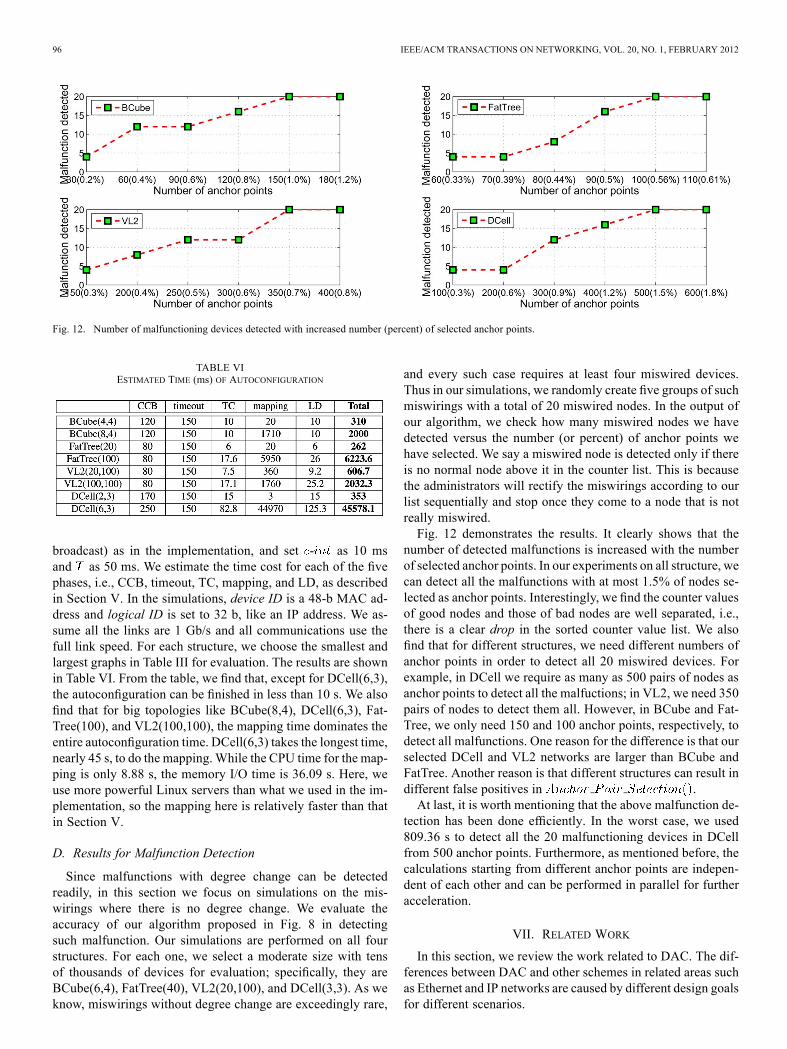
Fig. 12. Number of malfunctioning devices detected with increased number (percent) of selected anchor points.

TABLE VIESTIMATED TIME (ms) OF AUTOCONFIGURATION

broadcast) as in the implementation, and set - as 10 msand as 50 ms. We estimate the time cost for each of the fivephases, i.e., CCB, timeout, TC, mapping, and LD, as describedin Section V. In the simulations, device ID is a 48-b MAC ad-dress and logical ID is set to 32 b, like an IP address. We as-sume all the links are 1 Gb/s and all communications use thefull link speed. For each structure, we choose the smallest andlargest graphs in Table III for evaluation. The results are shownin Table VI. From the table, we find that, except for DCell(6,3),the autoconfiguration can be finished in less than 10 s. We alsofind that for big topologies like BCube(8,4), DCell(6,3), Fat-Tree(100), and VL2(100,100), the mapping time dominates theentire autoconfiguration time. DCell(6,3) takes the longest time,nearly 45 s, to do the mapping.While the CPU time for the map-ping is only 8.88 s, the memory I/O time is 36.09 s. Here, weuse more powerful Linux servers than what we used in the im-plementation, so the mapping here is relatively faster than thatin Section V.

D. Results for Malfunction Detection

Since malfunctions with degree change can be detectedreadily, in this section we focus on simulations on the mis-wirings where there is no degree change. We evaluate theaccuracy of our algorithm proposed in Fig. 8 in detectingsuch malfunction. Our simulations are performed on all fourstructures. For each one, we select a moderate size with tensof thousands of devices for evaluation; specifically, they areBCube(6,4), FatTree(40), VL2(20,100), and DCell(3,3). As weknow, miswirings without degree change are exceedingly rare,

and every such case requires at least four miswired devices.Thus in our simulations, we randomly create five groups of suchmiswirings with a total of 20 miswired nodes. In the output ofour algorithm, we check how many miswired nodes we havedetected versus the number (or percent) of anchor points wehave selected. We say a miswired node is detected only if thereis no normal node above it in the counter list. This is becausethe administrators will rectify the miswirings according to ourlist sequentially and stop once they come to a node that is notreally miswired.Fig. 12 demonstrates the results. It clearly shows that the

number of detected malfunctions is increased with the numberof selected anchor points. In our experiments on all structure, wecan detect all the malfunctions with at most 1.5% of nodes se-lected as anchor points. Interestingly, we find the counter valuesof good nodes and those of bad nodes are well separated, i.e.,there is a clear drop in the sorted counter value list. We alsofind that for different structures, we need different numbers ofanchor points in order to detect all 20 miswired devices. Forexample, in DCell we require as many as 500 pairs of nodes asanchor points to detect all the malfuctions; in VL2, we need 350pairs of nodes to detect them all. However, in BCube and Fat-Tree, we only need 150 and 100 anchor points, respectively, todetect all malfunctions. One reason for the difference is that ourselected DCell and VL2 networks are larger than BCube andFatTree. Another reason is that different structures can result indifferent false positives in .At last, it is worth mentioning that the above malfunction de-

tection has been done efficiently. In the worst case, we used809.36 s to detect all the 20 malfunctioning devices in DCellfrom 500 anchor points. Furthermore, as mentioned before, thecalculations starting from different anchor points are indepen-dent of each other and can be performed in parallel for furtheracceleration.

VII. RELATED WORK

In this section, we review the work related to DAC. The dif-ferences between DAC and other schemes in related areas suchas Ethernet and IP networks are caused by different design goalsfor different scenarios.


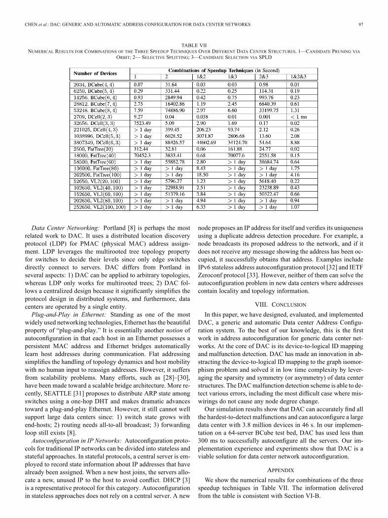
TABLE VIINUMERICAL RESULTS FOR COMBINATIONS OF THE THREE SPEEDUP TECHNIQUES OVER DIFFERENT DATA CENTER STRUCTURES. 1—CANDIDATE PRUNING VIA

ORBIT; 2— SELECTIVE SPLITTING; 3—CANDIDATE SELECTION VIA SPLD

Data Center Networking: Portland [8] is perhaps the mostrelated work to DAC. It uses a distributed location discoveryprotocol (LDP) for PMAC (physical MAC) address assign-ment. LDP leverages the multirooted tree topology propertyfor switches to decide their levels since only edge switchesdirectly connect to servers. DAC differs from Portland inseveral aspects: 1) DAC can be applied to arbitrary topologies,whereas LDP only works for multirooted trees; 2) DAC fol-lows a centralized design because it significantly simplifies theprotocol design in distributed systems, and furthermore, datacenters are operated by a single entity.Plug-and-Play in Ethernet: Standing as one of the most

widely used networking technologies, Ethernet has the beautifulproperty of “plug-and-play.” It is essentially another notion ofautoconfiguration in that each host in an Ethernet possesses apersistent MAC address and Ethernet bridges automaticallylearn host addresses during communication. Flat addressingsimplifies the handling of topology dynamics and host mobilitywith no human input to reassign addresses. However, it suffersfrom scalability problems. Many efforts, such as [28]–[30],have been made toward a scalable bridge architecture. More re-cently, SEATTLE [31] proposes to distribute ARP state amongswitches using a one-hop DHT and makes dramatic advancestoward a plug-and-play Ethernet. However, it still cannot wellsupport large data centers since: 1) switch state grows withend-hosts; 2) routing needs all-to-all broadcast; 3) forwardingloop still exists [8].Autoconfiguration in IP Networks: Autoconfiguration proto-

cols for traditional IP networks can be divided into stateless andstateful approaches. In stateful protocols, a central server is em-ployed to record state information about IP addresses that havealready been assigned. When a new host joins, the servers allo-cate a new, unused IP to the host to avoid conflict. DHCP [3]is a representative protocol for this category. Autoconfigurationin stateless approaches does not rely on a central server. A new

node proposes an IP address for itself and verifies its uniquenessusing a duplicate address detection procedure. For example, anode broadcasts its proposed address to the network, and if itdoes not receive any message showing the address has been oc-cupied, it successfully obtains that address. Examples includeIPv6 stateless address autoconfiguration protocol [32] and IETFZeroconf protocol [33]. However, neither of them can solve theautoconfiguration problem in new data centers where addressescontain locality and topology information.

VIII. CONCLUSION

In this paper, we have designed, evaluated, and implementedDAC, a generic and automatic Data center Address Configu-ration system. To the best of our knowledge, this is the firstwork in address autoconfiguration for generic data center net-works. At the core of DAC is its device-to-logical ID mappingand malfunction detection. DAC has made an innovation in ab-stracting the device-to-logical ID mapping to the graph isomor-phism problem and solved it in low time complexity by lever-aging the sparsity and symmetry (or asymmetry) of data centerstructures. TheDACmalfunction detection scheme is able to de-tect various errors, including the most difficult case where mis-wirings do not cause any node degree change.Our simulation results show that DAC can accurately find all

the hardest-to-detect malfunctions and can autoconfigure a largedata center with 3.8 million devices in 46 s. In our implemen-tation on a 64-server BCube test bed, DAC has used less than300 ms to successfully autoconfigure all the servers. Our im-plementation experience and experiments show that DAC is aviable solution for data center network autoconfiguration.

APPENDIX

We show the numerical results for combinations of the threespeedup techniques in Table VII. The information deliveredfrom the table is consistent with Section VI-B.


• Candidate pruning via orbit is very efficient for symmetricgraphs. For example, BCube is the most symmetric one ofall the evaluated structures, and the other technique combi-nations without candidate pruning via orbit all take longertime for BCube.

• Selective splitting is very efficient for sparse graphs. Forexample, we can see that with only selective splitting, overthe structures with a similar number of nodes, we haverelatively better results for DCell and VL2 (because theyare sparser), but relatively worse performance for BCubeand Fattree (because they are denser).

• Candidate selection via SPLD generally works togetherwith the other two techniques and can further improvethe performance when added, and the performance gain ismore obvious for asymmetric graphs such as DCell.

In the table, we do not consider the base algorithm withoutany speedup technique because it is extremely slow. We alsonote that we introduce the technique of candidate selection viaSPLD to work with the other two techniques. When using onlythis technique, the improvement over the baseline algorithmis quite limited for symmetric graphs such as BCube. In fact,the improvement from candidate pruning via orbit to candi-date pruning via orbit plus candidate selection via SPLD forBCube is mostly around two times in our experiments. This isbecause in very symmetric graphs, many devices have the sameSPLDs. We therefore do not further explore SPLD as a stand-alone speedup technique.

ACKNOWLEDGMENT

The authors thank G. Nordlund, W. Shen, and Y. Xu fortelling how IP addresses are assigned within MSRA researchdata center; G. Lu for test-bed setup; J. Zhou for his help oneducating them on the operation and miswiring issues in largecommercial data centers; X. Chen for helpful discussion onthe complexity of the general graph isomorphism problem.They thank the IEEE/ACM TRANSACTIONS ON NETWORKINGand SIGCOMM anonymous reviewers for their constructivecomments and their SIGCOMM shepherd M. Mitzenmacherfor his insightful and detailed feedback and suggestions, whichimproved the content and presentation of this paper.

REFERENCES

[1] R. H. Katz, “Tech titans building boom,” IEEE Spectrum, vol. 46, no.2, pp. 40–54, Feb. 2009.

[2] L. Barroso, J. Dean, and U. Hölzle, “Web search for a planet: TheGoogle cluster architecture,” IEEE Micro, vol. 23, no. 2, pp. 22–28,Mar. 2003.

[3] R. Droms, “Dynamic host configuration protocol,” RFC 2131, Mar.1997.

[4] S. Ghemawat, H. Gobioff, and S.-T. Leung, “The Google file system,”in Proc. ACM SOSP, 2003, pp. 29–43.

[5] J. Dean and S. Ghemawat, “MapReduce: Simplified data processing onlarge clusters,” in Proc. OSDI, 2004, pp. 137–150.

[6] C. Guo, H.Wu, K. Tan, L. Shi, Y. Zhang, and S. Lu, “DCell: A scalableand fault tolerant network structure for data centers,” in Proc. ACMSIGCOMM, 2008, pp. 75–86.

[7] C. Guo, G. Lu, D. Li, H. Wu, X. Zhang, Y. Shi, C. Tian, Y. Zhang,and S. Lu, “BCube: A high performance, server-centric network archi-tecture for modular data centers,” in Proc. ACM SIGCOMM, 2009, pp.63–74.

[8] R. N. Mysore, A. Pamboris, N. Farrington, N. Huang, P. Miri, S. Rad-hakrishnan, V. Subramanya, and A. Vahdat, “PortLand: A scalablefault-tolerant layer 2 data center network fabric,” in Proc. ACM SIG-COMM, 2009, pp. 39–50.

[9] A. Greenberg, N. Jain, S. Kandula, C. Kim, P. Lahiri, D.Maltz, P. Patel,and S. Sengupta, “VL2: A scalable and flexible data center network,”in Proc. ACM SIGCOMM, 2009, pp. 51–62.

[10] “Human errors most common reason for data center outages,”Oct. 2007 [Online]. Available: http://royal.pingdom.com/2007/10/30/human-errors-most-common-reason-for-data-center-outages

[11] Z. Kerravala, “As the value of enterprise networks escalates, so doesthe need for configuration management,” The Yankee Group, Boston,MA, Jan. 2004.

[12] “What’s behind network downtime?,” Juniper Networks, Sunnyvale,CA, 2008.

[13] R. McFarlane, “Where do failures originate?,” Nov. 2005 [On-line]. Available: http://searchdatacenter.techtarget.com/news/column/0,294698,sid80_gci1148903,00.html

[14] “GI problem,” [Online]. Available: http://en.wikipedia.org/wiki/Graph_isomorphism_problem

[15] B. D. McKay, “Practical graph isomorphism,” Cong. Numer., vol. 30,pp. 45–87, 1981.

[16] P. T. Darga, K. A. Sakallah, and I. L. Markov, “Faster symmetry dis-covery using sparsity of symmetries,” in Proc. 45th ACM/IEEE DesignAutom. Conf., 2008, pp. 149–154.

[17] D. Li, C. Guo, H. Wu, K. Tan, Y. Zhang, and S. Lu, “FiConn: Usingbackup port for server interconnection in data centers,” in Proc. IEEEINFOCOM, 2009, pp. 2276–2285.

[18] E. M. Luks, “Isomorphism of graphs of bounded valence can be testedin polynomial time,” J. Comput. Syst. Sci., vol. 25, no. 1, pp. 42–65,1982.

[19] “Graph automorphism,” [Online]. Available: http://en.wikipedia.org/wiki/Graph_automorphism

[20] K. Chen, C. Guo, H. Wu, J. Yuan, Z. Feng, Y. Chen, S. Lu, and W.Wu, “Generic and automatic address configuration for data center net-works,” MSR-TR-2011-62, 2011.

[21] P. T. Darga, M. H. Liffiton, K. A. Sakallah, and I. L. Markov, “Ex-ploiting structure in symmetry generation for CNF,” inProc. 41st ACM/IEEE Design Autom. Conf., 2004, pp. 530–534.

[22] “Data center network overview,” Extreme Networks, Santa Clara,CA, 2009 [Online]. Available: http://www.foss.ae/wp/wp-con-tent/uploads/downloads/info/Extreme/Data_Centre/Extreme%20Net-works-%20Data%20Centre%20Solution%20Overview.pdf

[23] “Maximum common subgraph problem,” [Online]. Available:http://en.wikipedia.org/wiki/Maximum_common_subgraph_isomor-phism_problem

[24] V. Kann, “On the approximability of the maximum common subgraphproblem,” in Proc. Annu. Symp. Theoret. Aspects Comput. Sci., 1992,pp. 377–388.

[25] C. Guo, Personal communications with operator of a large enterprisedata center, 2009.

[26] E. Kohler, R. Morris, B. Chen, J. Jannotti, and M. F. Kaashoek, “Theclickmodular router,” Trans. Comput. Syst., vol. 18, no. 3, pp. 263–297,2000.

[27] “DAC implementation,” Computer Science Department, North-western University, Evanston, IL, 2010 [Online]. Available:http://www.cs.northwestern.edu/~kch670/#software

[28] T. Rodeheffer, C. Thekkath, and D. Anderson, “SmartBridge: Ascalable bridge architecture,” in Proc. ACM SIGCOMM, 2000, pp.205–216.

[29] A.Myers, E. Ng, and H. Zhang, “Rethinking the service model: ScalingEthernet to a million nodes,” presented at the HotNets, 2004.

[30] R. Perlman, “Rbridges: Transparent routing,” in Proc. IEEE IN-FOCOM, 2004, vol. 2, pp. 1211–1218.

[31] C.Kim,M.Caesar, and J. Rexford, “Floodless in SEATTLE:A scalableethernet architecture for large enterprises,” in Proc. ACM SIGCOMM,2008, pp. 3–14.

[32] S. Thomson and T. Narten, “IPv6 stateless address autoconfiguration,”Expired Internet draft, Dec. 1998.

[33] S. Cheshire, B. Aboba, and E. Guttman, “Dynamic configuration ofIPv4 link-local addresses,” IETF draft, 2003.


Kai Chen received the B.S. and M.S. degrees incomputer science from the University of Scienceand Technology of China, Hefei, China, in 2004and 2007, respectively, and is currently pursuing thePh.D. degree in electrical engineering and computerscience at Northwestern University, Evanston, IL.He is interested in finding simple yet elegant solu-

tions to real networking and system problems.

Chuanxiong Guo received the Ph.D. degree fromNanjing Institute of Communications Engineering,Nanjing, China, in 2000.He is a Lead Researcher with the Wireless and

Networking Group, Microsoft Research Asia, Bei-jing, China. His research interests include networksystems design and analysis, data center networking,network security, networking support for operatingsystems, and cloud computing.

Haitao Wu (M’05) received the Bachelor’s degreein telecommunications engineering and the Ph.D. de-gree in telecommunications and information systemsfrom the Beijing University of Posts and Telecommu-nications (BUPT), Beijing, China, in 1998 and 2003,respectively.He joined the Wireless and Networking Group,

Microsoft Research Asia (MSRA), Beijing, China, in2003. His research interests are data center networks,QoS, TCP/IP, P2P, and wireless networks.

Jing Yuan received the B.S. degree from North-western Polytechnical University, Xi’an, China, in2005, and is currently pursuing the Ph.D. degreein automation at the Center for Intelligent andNetworked System, Tsinghua University, Beijing,China.Her research interests include network security,

network measurement and management, and datacenter networking.

Zhenqian Feng received the Bachelor’s andMaster’s degree in computer science and technologyfrom the National University of Defense Technology(NUDT), Changsha, China, in 2005 and 2008, re-spectively, and is currently pursuing the Ph.D. degreein computer science and technology at NUDT.His research interests include data center net-

works, TCP/IP, and network file systems.

Yan Chen received the Ph.D. degree in computer sci-ence from the University of California, Berkeley, in2003.He is an Associate Professor with the Department

of Electrical Engineering and Computer Science,Northwestern University, Evanston, IL. Based onGoogle Scholar, his papers have been cited over3600 times. His research interests include net-work security and measurement and diagnosis forlarge-scale networks and distributed systems.Dr. Chen won the Department of Energy (DoE)

Early CAREER Award in 2005, the Department of Defense (DoD) Young In-vestigator Award in 2007, and the Microsoft Trustworthy Computing Awards in2004 and 2005 with his colleagues.

Songwu Lu (S’95–M’00–SM’09) received theB.S. degree from the University of Science andTechnology of China, Hefei, China, in 1990, andthe M.S., and Ph.D. degrees from the University ofIllinois at Urbana–Champaign in 1996 and 1999,respectively.He is currently a Professor of computer science

with the University of California, Los Angeles(UCLA). His main research interests include wire-less networking, mobile systems, cloud computing,and network security.

WenfeiWu received the Bachelor’s degree fromBei-hang University, Beijing, China, in 2010, and is cur-rently a graduate student at the University of Wis-consin–Madison.He worked on data center autoconfiguration during

his internship with Microsoft Research Asia, Beijing,China.

84 IEEE/ACM TRANSACTIONS ON NETWORKING, VOL. …metro.cs.ucla.edu/papers/ton12-dac.pdf · errors...

Documents

Transcript of 84 IEEE/ACM TRANSACTIONS ON NETWORKING, VOL. …metro.cs.ucla.edu/papers/ton12-dac.pdf · errors...