835-2310
21
United States Environmental Protection Agency Prevention, Pesticides and Toxic Substances (7101) EPA 712–C–98–066 January 1998 Fate, Transport and Transformation Test Guidelines OPPTS 835.2310 Maximum Direct Photolysis Rate in Air from UV/Visible Spectroscopy
-
Upload
addin-akbar -
Category
Documents
-
view
214 -
download
0
description
FA
Transcript of 835-2310

United StatesEnvironmental ProtectionAgency
Prevention, Pesticidesand Toxic Substances(7101)
EPA 712–C–98–066January 1998
Fate, Transport andTransformation TestGuidelines
OPPTS 835.2310Maximum DirectPhotolysis Rate in Airfrom UV/VisibleSpectroscopy

i
INTRODUCTION
This guideline is one of a series of test guidelines that have beendeveloped by the Office of Prevention, Pesticides and Toxic Substances,United States Environmental Protection Agency for use in the testing ofpesticides and toxic substances, and the development of test data that mustbe submitted to the Agency for review under Federal regulations.
The Office of Prevention, Pesticides and Toxic Substances (OPPTS)has developed this guideline through a process of harmonization thatblended the testing guidance and requirements that existed in the Officeof Pollution Prevention and Toxics (OPPT) and appeared in Title 40,Chapter I, Subchapter R of the Code of Federal Regulations (CFR), theOffice of Pesticide Programs (OPP) which appeared in publications of theNational Technical Information Service (NTIS) and the guidelines pub-lished by the Organization for Economic Cooperation and Development(OECD).
The purpose of harmonizing these guidelines into a single set ofOPPTS guidelines is to minimize variations among the testing proceduresthat must be performed to meet the data requirements of the U. S. Environ-mental Protection Agency under the Toxic Substances Control Act (15U.S.C. 2601) and the Federal Insecticide, Fungicide and Rodenticide Act(7 U.S.C. 136, et seq.).
Final Guideline Release: This guideline is available from the U.S.Government Printing Office, Washington, DC 20402 on The Federal Bul-letin Board. By modem dial 202–512–1387, telnet and ftp:fedbbs.access.gpo.gov (IP 162.140.64.19), or call 202–512–0132 for disksor paper copies. This guideline is also available electronically in ASCIIand PDF (portable document format) from EPA’s World Wide Web site(http://www.epa.gov/epahome/research.htm) under the heading ‘‘Research-ers and Scientists/Test Methods and Guidelines/OPPTS Harmonized TestGuidelines.’’
1
OPPTS 835.2310 Maximum direct photolysis rate in air from UV/visi-ble spectroscopy.
(a) Scope—(1) Applicability. This guideline is intended to meet test-ing requirements of both the Federal Insecticide, Fungicide, andRodenticide Act (FIFRA) (7 U.S.C. 136, et seq.) and the Toxic SubstancesControl Act (TSCA) (15 U.S.C. 2601).
(2) Background. The source material used in developing this har-monized OPPTS test guideline is 40 CFR 796.3800 Gas Phase AbsorptionSpectra and Photolysis.
(b) Introduction—(1) Background and purpose. Numerous chemi-cals enter the atmosphere from a variety of sources. For example, chemi-cals enter the atmosphere as a result of the burning of coal, from the com-bustion of gasoline in cars and diesel fuel in trucks, and from the releaseof volatile organic chemicals during manufacture, processing, use, and dis-posal. Pesticides, applied from airplanes, enter the atmosphere directly andvolatilize from soils and water bodies. Chemical pollutants present in theatmosphere can undergo photochemical transformation in the environmentby direct photolysis in sunlight. Quantitative data in the form of rate con-stants and half-lives are needed to determine the importance of direct pho-tolysis of pollutants in the atmosphere. This test method describes a first-tier screening level test method to estimate the maximum direct photolysisrate constant and minimum half-life of chemicals in the atmosphere insunlight as a function of latitude and season of the year in the UnitedStates.
(2) Definitions and units. The definitions in section 3 of TSCA andin 40 CFR Part 792—Good Laboratory Practice Standards (GLP) applyto this test guideline. The following definitions also apply to this testguideline.
Absorbance (Aλ) is defined as the logarithm of the ratio of the initialintensity (I0) of a beam of radiant energy to the intensity (I) of the samebeam after passage through a sample at a fixed wavelength λ. Thus,Aλ = log (I0/I).
The actinic solar irradiance in the atmosphere (Jλ) is related to thesunlight intensity in the atmosphere and is proportional to the average lightflux (in units of photons per square centimer per day) that is availableto cause photoreaction in the wavelength interval ∆λ, centered at λ, overa 24–hour day at a specific latitude and season date. It is the irra-diance which would be measured by a weakly absorbing spherical acti-nometer exposed to direct solar radiation and sky radiation from all direc-tions.
The Beer-Lambert law states that the absorbance of a chemical inthe gas phase, at a fixed wavelength, is proportional to the thickness of
2
the absorbing material (l), or the light pathlength, and the concentrationof the absorbing species (C).
Cross section (σλ′) is defined as the proportionality constant in theBeer-Lambert law. Thus, Aλ = σλ′ Cl, where Aλ is the absorbance, Cis the concentration in molecules per cubic centimeter and l is thepathlength in centimeters. The units of the cross section σλ′ are squarecentimeters per molecule. Numerical values of the cross section dependupon the nature of the absorbing species.
Direct photolysis is defined as the direct absorption of light by achemical followed by a reaction which transforms the parent chemical intoone or more products.
A first-order reaction is defined as a reaction in which the rate ofdisappearance of a chemical is directly proportional to the concentrationof the chemical and is not a function of the concentration of any otherchemical present in the reaction mixture.
The Grotthus-Draper law, the first law of photochemistry, states thatonly light which is absorbed can be effective in producing a chemicaltransformation.
The half-life (t1/2) of a chemical is defined as the time required forthe concentration of the chemical being photolyzed to be reduced to one-half its initial value.
Radiant energy, or radiation, is defined as the energy traveling asa wave unaccompanied by transfer of matter. Examples include X-rays,visible light, UV light, radio waves, etc.
The reaction quantum yield (φλ) for an excited state process is de-fined as the fraction of absorbed light that results in photoreaction at afixed wavelength λ. It is the ratio of a number of molecules that photoreactto the number of quanta of light absorbed or the ratio of the number ofmoles that photoreact to the number of einsteins of light absorbed at afixed wavelength λ.
The Stark-Einstein law, the second law of photochemistry, states thatonly one molecule is activated to an excited state per photon or quantumof light absorbed.
The sunlight direct potolysis rate constant (kpE) is the first-order rateconstant (in units of day–1) and is a measure of the rate of disappearanceof a chemical in the gas phase in sunlight.
(3) Principle of the test method. (i) For weak absorbance of a chemi-cal in the atmosphere, the first-order direct photolysis rate constant, kpe,is given by the equation
3
Equation 1
kpE = 2.30 ¢λσ′λJλ
where φλ is the reaction quantum yield; φ′λ is the cross section (in unitsof cm2 molecule–1) averaged over a wavelength interval ∆λ, centered atλ; Jλ is the actinic solar irradiance (in units of photons cm–2 day–1) aver-aged over the wavelength interval ∆λ, centered at λ; and the summationis taken over the range ∆λ = 290 to 800 nm. Jλ is the solar actinic irradi-ance in the atmosphere under clear sky conditions and is a function oflatitude and season of the year.
(ii) Since this photolysis process is first-order, the half-life (t1/2) ofa chemical is given by
Equation 2
t1/2 = 0.693/kpe
(iii) A simple first-tier screening test has been developed using Equa-tion 1. As an approximation, it is assumed that the reaction quantum yieldφλ is equal to 1, the maximum value. As a result, the upper limit forthe direct photolysis sunlight rate constant in the gas phase is obtainedand Equation 1 becomes
Equation 3
(kpE)max = 2.30 Σσ′λJλ
Using Equation 3 in Equation 2, the lower limit for the half-life is givenby
Equation 4
(t1/2)min = 0.693/(kpE)max
The cross section can be determined experimentally by the procedures out-lined in paragraph (c) of this guideline and the values of Jλ are givenin Tables 1 to 4 under paragraph (c)(3) of this guideline as a functionof latitude and season of the year in the United States. These data canbe used in Equation 3 to calculate (kpE)max. Finally, (kpE)max can be sub-stituted in Equation 4 to calculate (t1/2)min.
(4) Applicability and specificity. (i) This test method is applicableto all chemicals which have UV/visible absorptions in the range 290 to800 nm. Some chemicals only have absorptions below 290 nm and con-sequently cannot undergo direct photolysis in sunlight (e.g. chemicals suchas alkanes, alkenes, alkynes, dienes, and fluoroalkanes).
4
(ii) This test method is only applicable to pure chemicals and notto the technical grade.
(iii) The first-tier screening test can be employed to estimate (kpE)max
and (t1/2)min. If these data indicate that gas phase photolysis is an importantprocess relative to other gas phase transformation processes (e.g. oxidationwith hydroxyl radicals or ozone), it is recommended that an upper-tierphotolysis test be carried out to determine the reaction quantum yield andthus obtain more precise environmentally relevant rate constants and half-lives in sunlight. The data obtained from this first-tier test method canbe used to determine (kpE)max for a test chemical as a function of latitudeand season of the year in the United States under clear sky conditions.These rate constants are in a form suitable for preliminary mathematicalmodeling for environmental fate of a test chemical.
(c) Test procedures. The procedures outlined in this test method arebased on the method proposed by Mill et al. under paragraph (e)(1) ofthis guideline and developed by Pitts et al. under paragraph (e)(2) of thisguideline. It is also recommended that OPPTS 830.7050 be consulted foradditional guidance.
(1) Test conditions—(i) UV/visible spectrophotometer. Althoughsingle-beam spectrophotometers may be used, recording double beamspectrophotometers are recommended. It is extremely important that thespectrophotometer be able to scan over the wavelength region 270 to 800nm and have an absorbance sensitivity, at a signal/noise ratio of one, ofapproximately 0.001. It is important that the spectrophotometer be ableto attain a 90 percent separation of two monochromatic spectral featuresapproximately 4 nm apart, peak to peak (i.e. the resolution should be atleast 4 nm). It is also desirable to have a spectrophotometer that can ac-commodate absorption cells of length ≥10 cm. A Cary 219 UV/VisibleSpectrophotometer, or an equivalent model, is recommended.
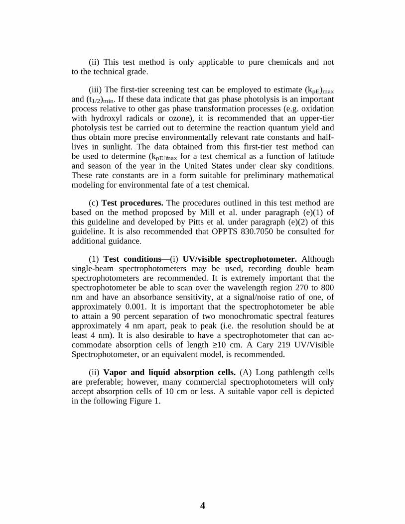
(ii) Vapor and liquid absorption cells. (A) Long pathlength cellsare preferable; however, many commercial spectrophotometers will onlyaccept absorption cells of 10 cm or less. A suitable vapor cell is depictedin the following Figure 1.
5
FIGURE 1—GAS ABSORPTION CELL
(B) A suitable vapor cell can be constructed as follows. The vaporcell should be constructed of Pyrex, 1 cm O.D. and 10 cm in length, andbe fitted with plane parallel quartz windows at each end. The quartz win-dows can be conveniently attached to the Pyrex cell with vaccum tightepoxy resin (e.g. Torr-Seal, Varian Associates) only applied to the outsidesurface. A Teflon stopcock (or a Pyrex O-ring stopcock) should be con-nected to the cell and contain an O-ring joint. The O-ring joint (e.g. no.7 or no. 9, Kontes or Ace Glass) must match the one on the vacuumrack. Viton O-rings are recommended and should be frequently inspectedfor signs of deterioration which would result in vacuum leaks. A matchedreference cell is extremely useful but not essential. However, the sampleand reference cells should be very similar. Small spectral differences be-tween the cells can be compensated for by running a blank with the sampleand reference cells in the spectrophotometer. The use of stopcock greaseis not required with these cells and should be avoided.
(C) A matched pair of liquid absorption cells is very desirable butis not essential. A pair of quartz UV absorption cells, 10 cm in length,having ground glass or Teflon stoppers are recommended. These liquidabsorption cells are readily available commercially.
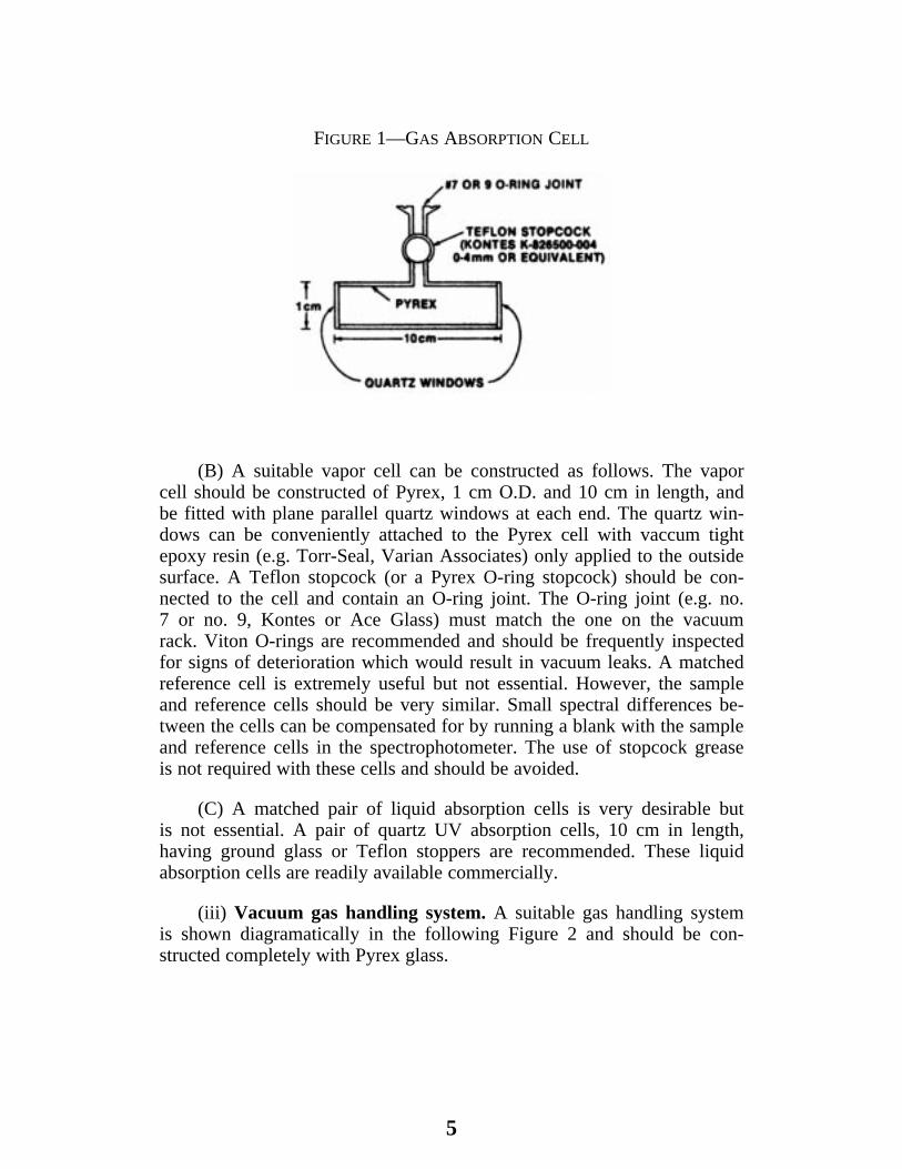
(iii) Vacuum gas handling system. A suitable gas handling systemis shown diagramatically in the following Figure 2 and should be con-structed completely with Pyrex glass.

6
FIGURE 2—SCHEMATIC OF GAS HANDLING VACUUM RACK
The components of the gas handling system are discussed below. The useof stopcock grease is not required and should be avoided.
(A) Vacuum pumping system. (1) In order to achieve a good vacu-um, i.e. pressures <10–5 torr (1.3 × 10⁻⁶ kPa), two pumps are required.The forepump (A) must be capable of achieving a pressure <0.05 torr(0.0065 kPa). A rotary pump (e.g. a Welch Model 1402 Duo-Seal or anequivalent model) is recommended. The forepump can be attached to thevacuum system by means of heavy-walled rubber vacuum tubing (B), orany flexible vacuum tubing. The exhaust from this pump should be ventedinto a hood.
(2) The second pump, a high vacuum model, should be a multistageoil diffusion pump (C) (e.g. a Consolidated Vacuum Corp. VMF–10 orVMF–20 or an equivalent model). The pump fluid should be a siliconeoil with a room temperature vapor pressure of ≤10–6 torr (1.3 × 10⁻⁷ kPa)(e.g. Dow-Corning D.C. 702 or 703, or an equivalent grade).

7
(3) It is extremely important that the pumping system contain a trap(D) cooled with liquid nitrogen. The cone and socket joint on this trapcan be conveniently sealed with Apiezon W wax, or an equivalent grade.This wax requires only gentle heating to apply and makes an effectivevacuum seal. It is possible that a few test chemicals could dissolveApiezon W wax. In this case, an inert silicone grease may be used toseal the trap.
(B) Vacuum rack. The recommended vacuum rack assembly is de-picted in Figure 2 under paragraph (d)(1)(iii) of this guideline. Allstopcocks should be of Teflon with Viton O-rings (Kontes K–826500 orK–826510 series or equivalent grades (or Pyrex O-ring stopcocks)). TheO-ring joints (E) (no. 7 or no. 9) must be compatible with those on thegas absorption cell (K) or on the liquid reservoir (J). These O-ring jointsshould be clamped by pinch clamps with a screw lock device (e.g. Thomas#18A, or an equivalent grade).
(C) Pressure Gauges. Three pressure gauges are required:
(1) An ionization gauge to measure high vacuum (<10–3 torr(1.3 × 10⁻⁴ kPa)).
(2) A thermocouple gauge to monitor the pressure in the range 10–3
to 1 torr (1.3 × 10⁻⁴ to 0.13 kPa). A convenient pressure monitoring systemwhich contains ionization and thermocouple gauges is a Consolidated Vac-uum Corp. Model GIC–300A or an equivalent model.
(3) A pressure gauge to monitor the pressure of the test chemicaland diluent in the range 0.01 to 760 torr (0.0013 to 101.3 kPa); for exam-ple, an MKS Baratron 310 BHS–1000 with the associated 170–6C elec-tronics unit and a digital readout or an equivalent model. While this vacu-um gauge exhibits a slow zero drift, it can be readily rezeroed using theionization gauge, i.e. when the ionization gauge reads approximately10–3 torr (0.00013 kPa) or less.
(2) Operation of the gas handling system. Since there are a widevariety of procedures available for operating a gas handling system, themethod used is left to the discretion of the tester. For those testers whodo not have experience in handling a vacuum system, the detailed proce-dure described in paragraph (d)(5) of this guideline is recommended.
(3) Preparation of samples—(i) Preparation of the gas phase testchemical sample: Preliminary Steps. (A) If the test chemical is a gasat room temperature, attach the gas container to the O-ring at the pointwhere the liquid reservoir (J) is placed. Close stopcocks 2 and 3 and open4. Pump until the pressure is <10–2 torr (1.3 × 10⁻³ kPa) as read on ther-mocouple gauge (H2). Then open stopcocks 2 and 3 and close 4 and pumpuntil the pressure is less than 10–5 torr (1.3 × 10⁻⁶ kPa) as read on theionization gauge (I).
8
(B) If the test chemical is a liquid at room temperature, add a fewcubic centimeters of liquid to a reservoir tube (J), sealed at one end andcontaining an O-ring at the other end, and connect the tube via the O-ring to stopcock 6. Freeze the sample with a Dewar containing liquid nitro-gen, close stopcocks 2 and 3 and open 4 and 6. Degas the test chemicalby allowing it to warm up to the liquid state, briefly degas, and refreezethe liquid. Repeat this process three or more times until the evolution ofgas bubbles ceases upon thawing. Freeze the liquid, open stopcocks 2 and3 and close 4. Pump until the pressure is less than 10–5 torr (1.3 × 10⁻⁶
kPa) as indicated by the ionization gauge (I). Close stopcock 6.
(ii) Introduction of the test chemical into the gas absorption cell.(A) For introduction of the test chemical into the gas absorption cell, closestopcocks 5, 7 and 10, with 9 and 11 open. If the test chemical is a gas,stopcock 6 should be opened and the gas container valve is graduallyopened to admit the gas into the gas handling manifold and gas absorptioncell until the desired pressure is attained, as read on the capacitance ma-nometer (G). Close the gas container valve and stopcock 6 and allow ap-proximately 5 min before the final pressure at (G) is read. If the pressurehas not stabilized in approximately 5 min allow the cell to condition forseveral hours before the final pressure at (G) is read.
(B) For a liquid chemical in the reservoir (J), which has beendegassed and is at liquid nitrogen temperature, the liquid nitrogen Dewarshould be removed and stopcock 6 opened. The cold liquid in the reservoir(J) is allowed to warm up until the required pressure is attained, as readby the capacitance manometer (G). Close stopcock 6 and cool the reservoiragain with liquid nitrogen and allow approximately 5 min before the finalpressure at (G) is read. If the pressure has not stabilized in approximately5 min, allow the cell to condition for several hours before the final pressureat (G) is read.
(C) With stopcocks 6, 8 and 11 closed and 5, 7, 9, and 10 open,the gas handling manifold is evacuated as described previously to a pres-sure less than 10–5 torr (1.3 × 10⁻⁶ kPa). Stopcocks 5 and 10 are thenclosed and ultra-high purity air from a cylinder is admitted into the gashandling manifold via stopcock 8 and through the trap (F) containing Mo-lecular Sieve 4A. When the manifold is at one atmosphere pressure, asmeasured by pressure gauge (G), stopcock 11 is briefly opened to pressurethe gas absorption cell to one atmosphere, and then closed. Stopcocks 8and 9 are closed and the gas handling system is evacuated as describedpreviously. The gas absorption cell can then be removed from (E) andcovered to avoid photolysis.
(D) Based on the pressure P of the test chemical, as measured bygauge (G), the concentration of the gas sample is
Equation 5

9
C (molecules cm–3) = 9.657 × 10¹⁸ P(torr)/T( K)
Equation 5a
C (molecules cm–3) = 1.287 × 10¹⁸ P(kPa)/T(K)
where T is the room temperature in degrees Kelvin, which should be rou-tinely monitored with a thermometer.
(F) The recommended pressure of the test chemical should be in therange 1–5 torr (0.13–0.65 kPa) where the Beer-Lambert law is obeyed.A final check on whether the test chemical obeys the Beer-Lambert lawcan be accomplished by demonstrating the constancy of the cross sectionat three partial pressures differing by a factor of 10.
(iii) Preparation of solution phase test chemical sample. (A) If theproperties of the test chemical (i.e. small cross sections, low vapor pres-sure) are such that the maximum absorbance obtainable is one-tenth ofthe most sensitive spectrophotometer scale or less (i.e. ≤0.001 absorbance),a solution-phase study should be undertaken. The most sensitive scale maybe limited by inherent spectrophotometer noise. For example, a givenspectrophotometer’s most sensitive scale is 0.00 to 0.10 absorbance units.Therefore, a test chemical for which the product of its maximum crosssection and its concentration is less than 0.001 (in a 10 cm cell) couldnot be analyzed in the vapor phase with this particular spectrophotometer.
(B) The following spectroscopic grade chemicals are recommendedto prepare solutions: chloroform, n-hexane, acetonitrile, and cyclohexane.Solutions of up to 10 percent by volume of test chemical can be preparedin one of these solvents in the standard manner.
(C) The concentration of the test chemical is given by the followingequations
Equation 6
C (molecules cm–3) = 6.022 × 10²³ mass (gms)/FW (Vd)
Equation 6a
C (molecules cm–3) = 6.022 × 10²³ Vsρ/FW (Vd)
where Vs is the volume of test chemical delivered into a volume Vd ofsolvent cubic centimeters, FW is the formula weight of the test chemicalin grams, and ρ is the density of the test chemical in grams per cubiccentimeter at the room temperature the solution was prepared.
(4) Procedure for obtaining the spectrum. As a general guide toobtaining UV/visible absorption spectra, the procedures outlined in OPPTS830.7050 are recommended. Since the method presented in this procedure

10
was developed by Pitts et al. (1981), it is recommended that this reportbe consulted for further details.
(i) Determination of the cell pathlength. The method for determin-ing the cell pathlength of gas or liquid cells is left to the discretion ofthe tester. However, the method listed in OPPTS 830.7050, using one ofthe reference compounds, is recommended.
(ii) Gas phase spectrum. Measure the absorbance of the test chemi-cal in duplicate relative to a matched cell filled with ultra-high purity airfrom the same cylinder similarly passed through trap (F) containing themolecular sieve. The absorbance should be measured at wavelengthsλ ≥ 280 nm using minimum slit widths. Record, in duplicate, the baselinewhen both the same reference cells are filled with high purity air driedthrough the molecular sieve and at the same settings as used for the testchemical sample. These data will be used to calculate the cross section,σ′λ, at the appropriate wavelength intervals, centered at wavelength λ, list-ed in Tables 1 through 4, under paragraph (d)(3) of this guideline.
(iii) Solution phase spectrum. (A) Measure the absorbance of thetest chemical in duplicate relative to a matched cell containing the solvent.The absorbance should be measured for wavelengths λ ≥ 280 nm usingthe minimum slit widths. Record, in duplicate, the baseline when both thesample and reference cells are filled with the solvents. These data willbe used to calculate the cross sections, σ′λ, for the appropriate wavelengthintervals, centered at λ, listed in Tables 1 through 4 under paragraph (d)(3)of this guideline.
(B) The concentration of the test chemical should be in the rangewhere the Beer-Lambert law is obeyed. A check on whether the test chemi-cal obeys this law can be accomplished by demonstrating the constancyof the cross section at three concentrations differing by a factor of 10.
(d) Data and reporting—(1) Treatment of results—(i) Determina-tion of the cross section from the gas phase spectrum. (A) The crosssection, σλ, can be determined from the gas phase absorption spectrumand the Beer-Lambert law in the form
Equation 7
σλ′ = Aλ/Cl
where Aλ is the absorbance at wavelength λ, centered in the wavelengthinterval >λ, C is the concentration of test chemical in molecules per cubiccentimeter, and l is the cell pathlength in centimeters. The cross sectionof the test chemical should be determined for the wavelength intervalslisted in Tables 1 through 4 under paragraph (d)(3) of this guideline.

11
(B) There are at least three nondestructive methods of determiningthe absorbance over a specified wavelength interval: estimation, squarecounting, and planimetry. For many spectra, estimating an averageabsorbance over a small wavelength interval is sufficient to yield accurateresults. However, for spectra containing rapidly changing absorptions andcomplex fine structure, square counting or planimetry should be used.These two methods require the integration of a definite region(in Aλ × nm) followed by division by the width of the region in nm toobtain absorbance. The method using a compensating polar planimeter isthe most accurate and is recommended. The absorbance should be obtainedfrom the average of three tracings.
(ii) Determination of the cross section from the solution phasespectrum. The cross section, σ′λ, can be determined from the solutionphase spectrum using Equation 7 for the wavelength intervals listed inTables 1 through 4 under paragraph (d)(3) of this guideline. For solutionspectra, estimating an average absorbance over the wavelength intervalsis sufficient to yield accurate results.
(iii) Estimation of the maximum direct photolysis rate constantand minimum half-life in the gas phase. (A) Using the cross sectionsobtained from the spectra and the values of Jλ from Tables 1–4 underparagraph (d)(3) of this guideline, the maximum direct photolysis rate con-stant (kpE)max can be calculated at a specific latitude and season for theyear using Equation 3. The minimum half-life, (t1/2E)min, can be calculatedusing this (kpE)max in Equation 4.
(B) An example is presented in under paragraph (d)(4) of this guide-line, to illustrate how the test data obtained in this section can be used.
(2) Test data report. (i) Submit the original chart, or photocopy,containing a plot of absorbance vs. wavelength plus the baseline. Spectrashould include a readable wavelength scale, preferably marked at 10 nmintervals. Each spectrum should be clearly marked.
(ii) Gas phase spectra. (A) Report the pressure of the test chemicalin torr (or kPa), the concentration in molecules per cubic centimeter, andthe pathlength of the sample cell in centimeters. Describe the method usedto determine the pathlength and report the experimental data.
(B) Report the wavelength λ, the wavelength interval for each10 nm over the region of absorption, the value of the absorbance (Aλ)for each replicate, the mean absorbance, and the mean cross section insquare centimeters per molecule.
(C) Report the estimated maximum direct photolysis rate constant inunits of reciprocal days and the corresponding minimum half-life in daysat 20°, 30°, 40°, and 50° north latitude for the summer and winter solstices.

12
(iii) Solution phase spectra. (A) Report the concentration of the testchemical in molecules per cubic centimeter, the type of cell used (quartzor borosilicate), and the pathlength in centimeters, the method used to de-termine the pathlength and report the experimental results.
(B) Report the identity of the solvent.
(C) Report the wavelength λ, the wavelength interval over the regionof absorption, the value of the absorbance (Aλ) of each replicate, the meanabsorbance, and the mean cross section square centimeter per molecule.
(D) Report the estimated maximum direct photolysis rate constant indays –1 and the corresponding minimum half-life in days at 20°, 30°, 40°,and 50° north latitude for the summer and winter solstices.
(iv) Report the name, structure, and purity of the test chemical.
(v) Submit a recent spectrum on appropriate reference chemicals forphotometric and wavelength accuracy.
(vi) Report the name and model of the spectrophotometer used.
(vii) Report the various control settings employed with thespectrophotometer. These might include scan speed, slit width, given, etc.
(viii) Report anything unusual about the test; e.g. if the Beer-Lambertlaw is not obeyed at a pressure of 1 to 5 torr (0.13 to 0.65 kPa), reportthe pressure at which the deviation was overcome and the experimentaldata. If the Beer-Lambert law is not obeyed in solution at high concentra-tions, report the concentration at which the deviation was overcome andthe experimental data.
(ix) Report any other relevant information.
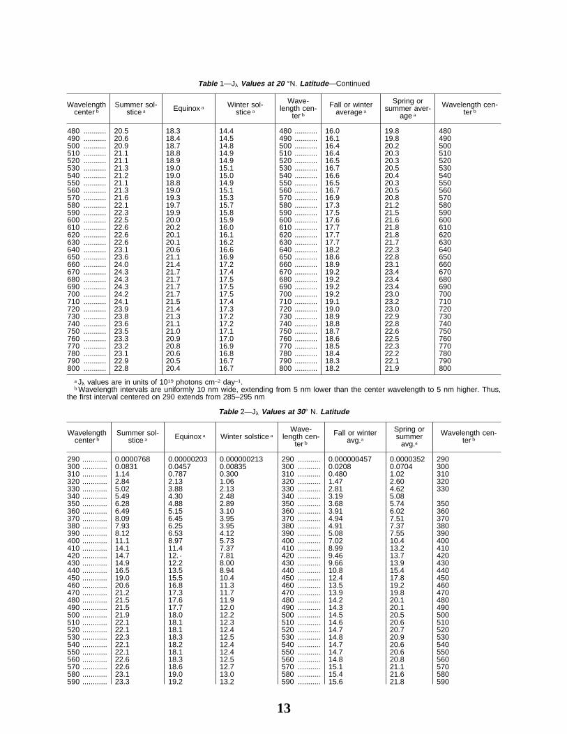
(3) Tables of solar irradianceTable 1—Jλ Values at 20 °N. Latitude
Wavelengthcenter b
Summer sol-stice a Equinox a Winter sol-
stice a
Wave-length cen-
ter b
Fall or winteraverage a
Spring orsummer aver-
age a
Wavelength cen-ter b
290 ........... 0.0000811 0.00000131 0.000000108 290 ........... 0.000000896 0.0000625 290300 ........... 0.0810 0.0611 0.0212 300 ........... 0.0359 0.0769 300310 ........... 1.10 0.9148 0.499 310 ........... 0.663 1.05 310320 ........... 2.74 2.35 1.52 320 ........... 1.855 2.62 320330 ........... 4.82 4.20 2.90 330 ........... 3.42 4.63 330340 ........... 5.27 4.61 3.28 340 ........... 3.82 5.06 340350 ........... 5.94 5.22 3.77 350 ........... 4.36 5.71 350360 ........... 6.22 5.47 4.01 360 ........... 4.61 5.98 360370 ........... 7.76 6.84 5.06 370 ........... 5.79 7.46 370380 ........... 7.60 6.71 5.02 380 ........... 5.71 7.31 380390 ........... 7.77 6.88 5.19 390 ........... 5.88 7.48 390400 ........... 10.6 9.44 7.17 400 ........... 8.10 10.2 400410 ........... 13.5 12.0 9.17 410 ........... 10.3 13.0 410420 ........... 14.1 12.5 9.65 420 ........... 10.8 13.6 420430 ........... 14.3 12.7 9.85 430 ........... 11.1 13.7 430440 ........... 15.8 14.1 11.0 440 ........... 12.2 15.2 440450 ........... 18.2 16.2 12.7 450 ........... 14.1 17.5 450460 ........... 19.7 17.5 13.7 460 ........... 15.3 18.9 460470 ........... 20.2 18.1 14.2 470 ........... 15.8 19.5 470
13
Table 1—Jλ Values at 20 °N. Latitude—Continued
Wavelengthcenter b
Summer sol-stice a Equinox a Winter sol-
stice a
Wave-length cen-
ter b
Fall or winteraverage a
Spring orsummer aver-
age a
Wavelength cen-ter b
480 ........... 20.5 18.3 14.4 480 ........... 16.0 19.8 480490 ........... 20.6 18.4 14.5 490 ........... 16.1 19.8 490500 ........... 20.9 18.7 14.8 500 ........... 16.4 20.2 500510 ........... 21.1 18.8 14.9 510 ........... 16.4 20.3 510520 ........... 21.1 18.9 14.9 520 ........... 16.5 20.3 520530 ........... 21.3 19.0 15.1 530 ........... 16.7 20.5 530540 ........... 21.2 19.0 15.0 540 ........... 16.6 20.4 540550 ........... 21.1 18.8 14.9 550 ........... 16.5 20.3 550560 ........... 21.3 19.0 15.1 560 ........... 16.7 20.5 560570 ........... 21.6 19.3 15.3 570 ........... 16.9 20.8 570580 ........... 22.1 19.7 15.7 580 ........... 17.3 21.2 580590 ........... 22.3 19.9 15.8 590 ........... 17.5 21.5 590600 ........... 22.5 20.0 15.9 600 ........... 17.6 21.6 600610 ........... 22.6 20.2 16.0 610 ........... 17.7 21.8 610620 ........... 22.6 20.1 16.1 620 ........... 17.7 21.8 620630 ........... 22.6 20.1 16.2 630 ........... 17.7 21.7 630640 ........... 23.1 20.6 16.6 640 ........... 18.2 22.3 640650 ........... 23.6 21.1 16.9 650 ........... 18.6 22.8 650660 ........... 24.0 21.4 17.2 660 ........... 18.9 23.1 660670 ........... 24.3 21.7 17.4 670 ........... 19.2 23.4 670680 ........... 24.3 21.7 17.5 680 ........... 19.2 23.4 680690 ........... 24.3 21.7 17.5 690 ........... 19.2 23.4 690700 ........... 24.2 21.7 17.5 700 ........... 19.2 23.0 700710 ........... 24.1 21.5 17.4 710 ........... 19.1 23.2 710720 ........... 23.9 21.4 17.3 720 ........... 19.0 23.0 720730 ........... 23.8 21.3 17.2 730 ........... 18.9 22.9 730740 ........... 23.6 21.1 17.2 740 ........... 18.8 22.8 740750 ........... 23.5 21.0 17.1 750 ........... 18.7 22.6 750760 ........... 23.3 20.9 17.0 760 ........... 18.6 22.5 760770 ........... 23.2 20.8 16.9 770 ........... 18.5 22.3 770780 ........... 23.1 20.6 16.8 780 ........... 18.4 22.2 780790 ........... 22.9 20.5 16.7 790 ........... 18.3 22.1 790800 ........... 22.8 20.4 16.7 800 ........... 18.2 21.9 800
a Jλ values are in units of 1019 photons cm–2 day–1.b Wavelength intervals are uniformly 10 nm wide, extending from 5 nm lower than the center wavelength to 5 nm higher. Thus,
the first interval centered on 290 extends from 285–295 nm
Table 2—Jλ Values at 30° N. Latitude
Wavelengthcenter b
Summer sol-stice a Equinox a Winter solstice a
Wave-length cen-
ter b
Fall or winteravg.a
Spring orsummer
avg.aWavelength cen-
ter b
290 ............ 0.0000768 0.00000203 0.000000213 290 ........... 0.000000457 0.0000352 290300 ............ 0.0831 0.0457 0.00835 300 ........... 0.0208 0.0704 300310 ............ 1.14 0.787 0.300 310 ........... 0.480 1.02 310320 ............ 2.84 2.13 1.06 320 ........... 1.47 2.60 320330 ............ 5.02 3.88 2.13 330 ........... 2.81 4.62 330340 ............ 5.49 4.30 2.48 340 ........... 3.19 5.08350 ............ 6.28 4.88 2.89 350 ........... 3.68 5.74 350360 ............ 6.49 5.15 3.10 360 ........... 3.91 6.02 360370 ............ 8.09 6.45 3.95 370 ........... 4.94 7.51 370380 ............ 7.93 6.25 3.95 380 ........... 4.91 7.37 380390 ............ 8.12 6.53 4.12 390 ........... 5.08 7.55 390400 ............ 11.1 8.97 5.73 400 ........... 7.02 10.4 400410 ............ 14.1 11.4 7.37 410 ........... 8.99 13.2 410420 ............ 14.7 12.· 7.81 420 ........... 9.46 13.7 420430 ............ 14.9 12.2 8.00 430 ........... 9.66 13.9 430440 ............ 16.5 13.5 8.94 440 ........... 10.8 15.4 440450 ............ 19.0 15.5 10.4 450 ........... 12.4 17.8 450460 ............ 20.6 16.8 11.3 460 ........... 13.5 19.2 460470 ............ 21.2 17.3 11.7 470 ........... 13.9 19.8 470480 ............ 21.5 17.6 11.9 480 ........... 14.2 20.1 480490 ............ 21.5 17.7 12.0 490 ........... 14.3 20.1 490500 ............ 21.9 18.0 12.2 500 ........... 14.5 20.5 500510 ............ 22.1 18.1 12.3 510 ........... 14.6 20.6 510520 ............ 22.1 18.1 12.4 520 ........... 14.7 20.7 520530 ............ 22.3 18.3 12.5 530 ........... 14.8 20.9 530540 ............ 22.1 18.2 12.4 540 ........... 14.7 20.6 540550 ............ 22.1 18.1 12.4 550 ........... 14.7 20.6 550560 ............ 22.6 18.3 12.5 560 ........... 14.8 20.8 560570 ............ 22.6 18.6 12.7 570 ........... 15.1 21.1 570580 ............ 23.1 19.0 13.0 580 ........... 15.4 21.6 580590 ............ 23.3 19.2 13.2 590 ........... 15.6 21.8 590

14
Table 2—Jλ Values at 30° N. Latitude—Continued
Wavelengthcenter b
Summer sol-stice a Equinox a Winter solstice a
Wave-length cen-
ter b
Fall or winteravg.a
Spring orsummer
avg.aWavelength cen-
ter b
600 ............ 23.5 19.3 13.3 600 ........... 15.7 22.0 600610 ............ 23.7 19.5 13.4 610 ........... 15.8 22.1 610620 ............ 23.6 19.3 13.6 620 ........... 15.9 22.1 620630 ............ 23.6 19.2 13.7 630 ........... 16.0 22.1 630640 ............ 24.2 19.8 14.0 640 ........... 16.3 22.6 640650 ............ 24.7 20.4 14.2 650 ........... 16.7 23.1 650660 ............ 25.1 20.7 14.4 660 ........... 16.9 23.5 660670 ............ 25.4 21.0 14.7 670 ........... 17.2 23.8 670680 ............ 25.4 21.0 14.7 680 ........... 17.2 23.8 680690 ............ 25.4 21.0 14.8 690 ........... 17.3 23.8 690700 ............ 25.3 21.0 14.8 700 ........... 17.3 23.7 700710 ............ 25.2 20.8 14.7 710 ........... 17.2 23.6 710720 ............ 25.0 20.7 14.6 720 ........... 17.1 23.4 720730 ............ 24.9 20.6 14.6 730 ........... 17.0 23.3 730740 ............ 24.7 20.5 14.5 740 ........... 16.9 23.2 740750 ............ 24.6 20.4 14.5 750 ........... 16.8 23.0 750760 ............ 24.4 20.3 14.4 760 ........... 16.8 22.9 760770 ............ 24.3 20.1 14.3 770 ........... 16.7 22.7 770780 ............ 24.1 20.0 14.3 780 ........... 16.6 22.6 780790 ............ 24.0 19.9 14.2 790 ........... 16.5 22.5 790800 ............ 23.8 19.8 14.2 800 ........... 16.4 22.3 800
aJλ values are in units of 1019 photons cm–2 day–1.b Wavelength intervals are uniformly 10 nm wide, extending from 5 nm lower than the center wavelength to 5 nm higher. Thus,
the first interval centered on 290 extends from 285–295 nm
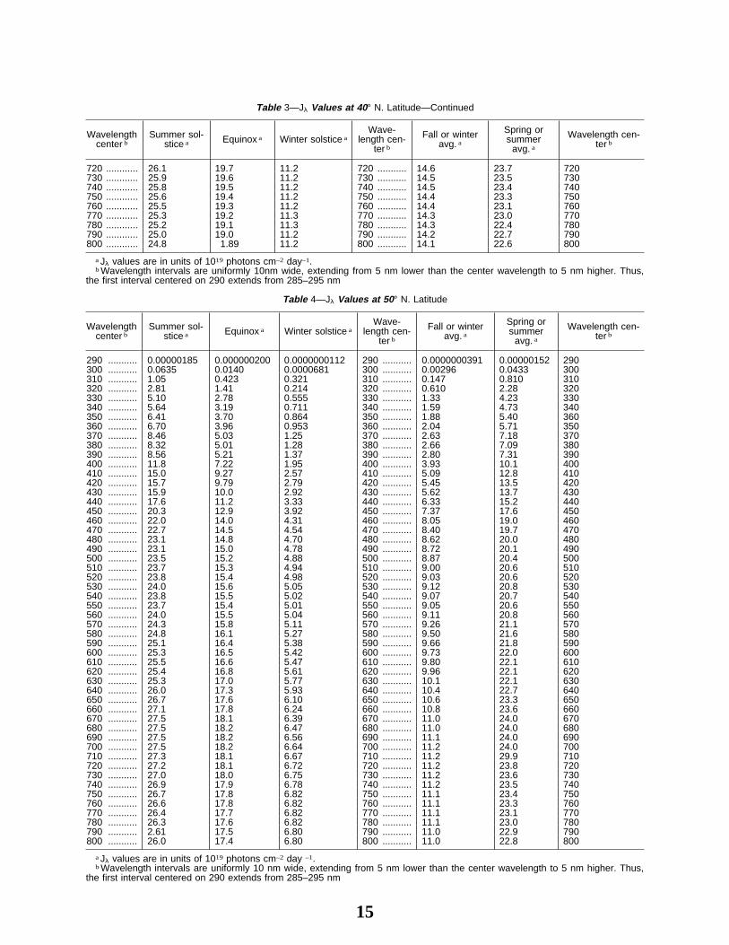
Table 3—Jλ Values at 40° N. Latitude
Wavelengthcenter b
Summer sol-stice a Equinox a Winter solstice a
Wave-length cen-
ter b
Fall or winteravg. a
Spring orsummer
avg. a
Wavelength cen-ter b
290 ............ 1.36 × 10⁻⁵ 1.21 × 10⁻⁷ 6.15 × 10⁻¹⁰ 290 ........... 8.14 × 10⁻⁸ 3.49 × 10⁻⁶ 290300 ............ 0.0769 0.0293 0.00145 300 ........... 0.00939 0.0587 300310 ............ 1.12 0.618 0.132 310 ........... 0.298 0.940 310320 ............ 2.87 1.81 0.591 320 ........... 1.04 2.49 320330 ............ 5.11 3.41 1.31 330 ........... 2.90 4.49 330340 ............ 5.62 3.83 1.58 340 ........... 2.43 4.77 340350 ............ 6.35 4.39 1.88 350 ........... 2.84 5.64 350360 ............ 6.61 4.65 2.05 360 ........... 3.05 5.93 360370 ............ 8.32 5.86 2.64 370 ........... 3.88 7.43 370380 ............ 8.17 5.80 2.67 380 ........... 3.88 7.30 380390 ............ 8.37 5.99 2.82 390 ........... 4.05 7.50 390400 ............ 11.5 8.26 3.97 400 ........... 5.64 10.3 400410 ............ 14.6 10.5 5.15 410 ........... 7.26 13.1 410420 ............ 15.2 11.1 5.51 420 ........... 7.69 13.9 420430 ............ 15.5 11.3 6.69 430 ........... 7.89 15.4 430440 ............ 17.1 12.5 6.41 440 ........... 8.82 17.8 440450 ............ 19.7 14.5 7.47 450 ........... 10.2 19.2 450460 ............ 21.3 15.7 8.15 460 ........... 11.1 19.8 460470 ............ 22.0 16.2 8.51 470 ........... 11.5 20.1 470480 ............ 22.3 16.5 8.74 480 ........... 11.8 20.2 480490 ............ 22.3 16.6 8.83 490 ........... 11.9 20.6 490500 ............ 22.7 16.9 8.99 500 ........... 12.1 20.7 500510 ............ 22.9 17.0 9.07 510 ........... 12.2 20.8 510520 ............ 22.9 17.0 9.14 520 ........... 12.3 21.0 520530 ............ 23.2 17.2 9.24 530 ........... 12.4 21.0 530540 ............ 23.0 17.1 9.18 540 ........... 12.3 20.8 540550 ............ 22.9 17.0 9.15 550 ........... 12.3 20.7 550560 ............ 23.1 17.2 9.23 560 ........... 12.4 20.9 560570 ............ 23.5 17.4 9.38 570 ........... 12.6 21.2 570580 ............ 24.0 17.8 9.62 580 ........... 12.9 21.9 580590 ............ 24.2 18.0 9.79 590 ........... 13.1 21.9 590600 ............ 24.4 18.2 9.85 600 ........... 13.2 22.1 600610 ............ 24.6 18.3 9.93 610 ........... 13.2 22.2 610620 ............ 24.5 18.3 10.2 620 ........... 13.4 22.2 620630 ............ 24.5 18.3 10.2 630 ........... 13.5 22.1 630640 ............ 25.1 18.8 10.5 640 ........... 13.8 22.7 640650 ............ 25.7 19.2 10.7 650 ........... 14.1 23.3 650660 ............ 26.1 19.5 10.9 660 ........... 14.3 23.6 660670 ............ 26.4 19.8 11.1 670 ........... 14.5 24.0 670680 ............ 26.3 19.9 11.1 680 ........... 14.6 24.0 680690 ............ 26.4 19.9 11.2 690 ........... 14.6 24.0 690700 ............ 26.4 19.9 11.3 700 ........... 14.7 24.0 700710 ............ 26.2 19.8 11.2 710 ........... 14.6 23.9 710
15
Table 3—Jλ Values at 40° N. Latitude—Continued
Wavelengthcenter b
Summer sol-stice a Equinox a Winter solstice a
Wave-length cen-
ter b
Fall or winteravg. a
Spring orsummer
avg. a
Wavelength cen-ter b
720 ............ 26.1 19.7 11.2 720 ........... 14.6 23.7 720730 ............ 25.9 19.6 11.2 730 ........... 14.5 23.5 730740 ............ 25.8 19.5 11.2 740 ........... 14.5 23.4 740750 ............ 25.6 19.4 11.2 750 ........... 14.4 23.3 750760 ............ 25.5 19.3 11.2 760 ........... 14.4 23.1 760770 ............ 25.3 19.2 11.3 770 ........... 14.3 23.0 770780 ............ 25.2 19.1 11.3 780 ........... 14.3 22.4 780790 ............ 25.0 19.0 11.2 790 ........... 14.2 22.7 790800 ............ 24.8 1.89 11.2 800 ........... 14.1 22.6 800
a Jλ values are in units of 1019 photons cm–2 day–1.b Wavelength intervals are uniformly 10nm wide, extending from 5 nm lower than the center wavelength to 5 nm higher. Thus,
the first interval centered on 290 extends from 285–295 nm
Table 4—Jλ Values at 50° N. Latitude
Wavelengthcenter b
Summer sol-stice a Equinox a Winter solstice a
Wave-length cen-
ter b
Fall or winteravg. a
Spring orsummer
avg. a
Wavelength cen-ter b
290 ........... 0.00000185 0.000000200 0.0000000112 290 ........... 0.0000000391 0.00000152 290300 ........... 0.0635 0.0140 0.0000681 300 ........... 0.00296 0.0433 300310 ........... 1.05 0.423 0.321 310 ........... 0.147 0.810 310320 ........... 2.81 1.41 0.214 320 ........... 0.610 2.28 320330 ........... 5.10 2.78 0.555 330 ........... 1.33 4.23 330340 ........... 5.64 3.19 0.711 340 ........... 1.59 4.73 340350 ........... 6.41 3.70 0.864 350 ........... 1.88 5.40 360360 ........... 6.70 3.96 0.953 360 ........... 2.04 5.71 350370 ........... 8.46 5.03 1.25 370 ........... 2.63 7.18 370380 ........... 8.32 5.01 1.28 380 ........... 2.66 7.09 380390 ........... 8.56 5.21 1.37 390 ........... 2.80 7.31 390400 ........... 11.8 7.22 1.95 400 ........... 3.93 10.1 400410 ........... 15.0 9.27 2.57 410 ........... 5.09 12.8 410420 ........... 15.7 9.79 2.79 420 ........... 5.45 13.5 420430 ........... 15.9 10.0 2.92 430 ........... 5.62 13.7 430440 ........... 17.6 11.2 3.33 440 ........... 6.33 15.2 440450 ........... 20.3 12.9 3.92 450 ........... 7.37 17.6 450460 ........... 22.0 14.0 4.31 460 ........... 8.05 19.0 460470 ........... 22.7 14.5 4.54 470 ........... 8.40 19.7 470480 ........... 23.1 14.8 4.70 480 ........... 8.62 20.0 480490 ........... 23.1 15.0 4.78 490 ........... 8.72 20.1 490500 ........... 23.5 15.2 4.88 500 ........... 8.87 20.4 500510 ........... 23.7 15.3 4.94 510 ........... 9.00 20.6 510520 ........... 23.8 15.4 4.98 520 ........... 9.03 20.6 520530 ........... 24.0 15.6 5.05 530 ........... 9.12 20.8 530540 ........... 23.8 15.5 5.02 540 ........... 9.07 20.7 540550 ........... 23.7 15.4 5.01 550 ........... 9.05 20.6 550560 ........... 24.0 15.5 5.04 560 ........... 9.11 20.8 560570 ........... 24.3 15.8 5.11 570 ........... 9.26 21.1 570580 ........... 24.8 16.1 5.27 580 ........... 9.50 21.6 580590 ........... 25.1 16.4 5.38 590 ........... 9.66 21.8 590600 ........... 25.3 16.5 5.42 600 ........... 9.73 22.0 600610 ........... 25.5 16.6 5.47 610 ........... 9.80 22.1 610620 ........... 25.4 16.8 5.61 620 ........... 9.96 22.1 620630 ........... 25.3 17.0 5.77 630 ........... 10.1 22.1 630640 ........... 26.0 17.3 5.93 640 ........... 10.4 22.7 640650 ........... 26.7 17.6 6.10 650 ........... 10.6 23.3 650660 ........... 27.1 17.8 6.24 660 ........... 10.8 23.6 660670 ........... 27.5 18.1 6.39 670 ........... 11.0 24.0 670680 ........... 27.5 18.2 6.47 680 ........... 11.0 24.0 680690 ........... 27.5 18.2 6.56 690 ........... 11.1 24.0 690700 ........... 27.5 18.2 6.64 700 ........... 11.2 24.0 700710 ........... 27.3 18.1 6.67 710 ........... 11.2 29.9 710720 ........... 27.2 18.1 6.72 720 ........... 11.2 23.8 720730 ........... 27.0 18.0 6.75 730 ........... 11.2 23.6 730740 ........... 26.9 17.9 6.78 740 ........... 11.2 23.5 740750 ........... 26.7 17.8 6.82 750 ........... 11.1 23.4 750760 ........... 26.6 17.8 6.82 760 ........... 11.1 23.3 760770 ........... 26.4 17.7 6.82 770 ........... 11.1 23.1 770780 ........... 26.3 17.6 6.82 780 ........... 11.1 23.0 780790 ........... 2.61 17.5 6.80 790 ........... 11.0 22.9 790800 ........... 26.0 17.4 6.80 800 ........... 11.0 22.8 800
a Jλ values are in units of 1019 photons cm–2 day –1.b Wavelength intervals are uniformly 10 nm wide, extending from 5 nm lower than the center wavelength to 5 nm higher. Thus,
the first interval centered on 290 extends from 285–295 nm
16
(4) Example of application of methodology. (i) Consider a chemicalplant located in Freeport, Texas, which produces acrolein (CH2=CHCHO)continuously every day of the year. Despite the fact that all acroleinwastes, including vented vapors, are treated in a waste-treatment plant,some acrolein escapes into the atmosphere. The chemical plant is locatedat 29° north latitude. Estimate the maximum sunlight direct photolysis rateconstant and the corresponding minimum half-life in the atmosphere inthe vicinity of the plant for the winter and summer season solstices underclear sky conditions.
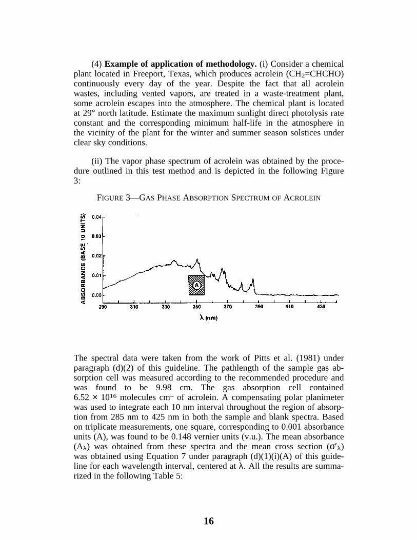
(ii) The vapor phase spectrum of acrolein was obtained by the proce-dure outlined in this test method and is depicted in the following Figure3:
FIGURE 3—GAS PHASE ABSORPTION SPECTRUM OF ACROLEIN
The spectral data were taken from the work of Pitts et al. (1981) underparagraph (d)(2) of this guideline. The pathlength of the sample gas ab-sorption cell was measured according to the recommended procedure andwas found to be 9.98 cm. The gas absorption cell contained6.52 × 1016 molecules cm– of acrolein. A compensating polar planimeterwas used to integrate each 10 nm interval throughout the region of absorp-tion from 285 nm to 425 nm in both the sample and blank spectra. Basedon triplicate measurements, one square, corresponding to 0.001 absorbanceunits (A), was found to be 0.148 vernier units (v.u.). The mean absorbance(Aλ) was obtained from these spectra and the mean cross section (σ′λ)was obtained using Equation 7 under paragraph (d)(1)(i)(A) of this guide-line for each wavelength interval, centered at λ. All the results are summa-rized in the following Table 5:

17
Table 5—Absorbance and Cross Section for Acrolein Vapor 1
Wavelength λ (nm) Wavelength interval (nm) Mean absorbance (Aλ) Mean cross section σ′λ)(cm2 molecule–1)
290 ...................................... 285–295 0.0037 5.69 × 10⁻²¹
300 ...................................... 295–305 0.0066 1.01 × 10⁻²⁰
310 ...................................... 305–315 0.0104 1.60 × 10⁻²⁰
320 ...................................... 315–325 0.0137 2.11 × 10⁻²⁰
330 ...................................... 325–335 0.0156 2.40 × 10⁻²⁰
340 ...................................... 335–345 0.0156 2.40 × 10⁻²⁰
350 ...................................... 345–355 0.0151 2.32 × 10⁻²⁰
360 ...................................... 355–365 0.0096 1.48 × 10⁻²⁰
370 ...................................... 365–375 0.0073 1.12 × 10⁻²⁰
380 ...................................... 375–385 0.0031 4.76 × 10⁻²¹
390 ...................................... 385–395 0.0016 2.46 × 10⁻²¹
400 ...................................... 395–405 0.0004 6.15 × 10⁻²²
410 ...................................... 405–415 0.0003 4.61 × 10⁻²²
420 ...................................... 415–425 0.0000 0.00
1 6.52 × 10¹⁶ molecules cm–3 in a 9.98 cm gas absorption cell
(iii) A sample calculation is given for the wavelength λ = 305 nm,centered over the wavelength interval 345 to 355 nm. For convenience,the area A, corresponding to 100 squares was blocked off in this absorp-tion area and was not integrated with the planimeter. The average vernierreading of the remaining absorption area was 7.2 v.u. Hence,
7.2 v.u./(0.148 v.u./square) = 49 squares
and the total area in the spectrum in the wavelength interval 345 to 355,centered at λ = 350 nm, is 149 squares. This number of squares cor-responds to 0.0149 absorbance units:
(149 squares)(0.001 A/square)/10 = 0.0149 A
From the blank spectrum, the baseline absorbance (Aλ blank) over thisinterval was –0.0001. The sample trace lay at ·0.0001 absorbance unitsrelative to a zero point at 450 nm. The observed sample absorbance isthen equal to 0.0150 (0.0149 + 0.0001). The absolute corrected absorbancefor the sample is given by
Acorrλsample = Aobsλsample – Aλblank
Acorrλsample = 0.0150 – (–0.001) = 0.0151 A
(iv) Using Equation 7 under paragraph (d)(1)(i)(A) of this guidelineand the values for the corrected sample absorbance, l, and C, the meancross section for the wavelength λ = 350 nm, centered over the wavelengthinterval 345–355 nm, is
σ′λ = 0.0151/(6.52 × 1016 molecules cm–3) (9.98cm)
= 2.3 × 10⁻²⁰ cm2molecule–1
(v) Since the plant is located at 29° north latitude, the closest Jλ val-ues are at 30° north latitude. These values are obtained from Table 2 under
18
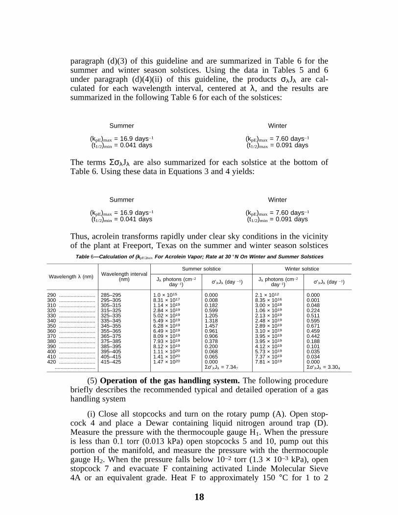
paragraph (d)(3) of this guideline and are summarized in Table 6 for thesummer and winter season solstices. Using the data in Tables 5 and 6under paragraph (d)(4)(ii) of this guideline, the products σλJλ are cal-culated for each wavelength interval, centered at λ, and the results aresummarized in the following Table 6 for each of the solstices:
Summer Winter
(kpE)max = 16.9 days–1 (kpE)max = 7.60 days–1
(t1/2)min = 0.041 days (t1/2)max = 0.091 days
The terms ΣσλJλ are also summarized for each solstice at the bottom ofTable 6. Using these data in Equations 3 and 4 yields:
Summer Winter
(kpE)max = 16.9 days–1 (kpE)max = 7.60 days–1
(t1/2)min = 0.041 days (t1/2)min = 0.091 days
Thus, acrolein transforms rapidly under clear sky conditions in the vicinityof the plant at Freeport, Texas on the summer and winter season solstices
Table 6—Calculation of (kpE)max For Acrolein Vapor; Rate at 30 °N On Winter and Summer Solstices
Wavelength λ (nm) Wavelength interval(nm)
Summer solstice Winter solstice
Jλ photons (cm–2
day–1) σ′λJλ (day –1) Jλ photons (cm–2
day–1) σ′λJλ (day –1)
290 ......................... 285–295 1.0 × 10¹⁵ 0.000 2.1 × 10¹² 0.000300 ......................... 295–305 8.31 × 10¹⁷ 0.008 8.35 × 10¹⁶ 0.001310 ......................... 305–315 1.14 × 10¹⁹ 0.182 3.00 × 10¹⁸ 0.048320 ......................... 315–325 2.84 × 10¹⁹ 0.599 1.06 × 10¹⁹ 0.224330 ......................... 325–335 5.02 × 10¹⁹ 1.205 2.13 × 10¹⁹ 0.511340 ......................... 335–345 5.49 × 10¹⁹ 1.318 2.48 × 10¹⁹ 0.595350 ......................... 345–355 6.28 × 10¹⁹ 1.457 2.89 × 10¹⁹ 0.671360 ......................... 355–365 6.49 × 10¹⁹ 0.961 3.10 × 10¹⁹ 0.459370 ......................... 365–375 8.09 × 10¹⁹ 0.906 3.95 × 10¹⁹ 0.442380 ......................... 375–385 7.93 × 10¹⁹ 0.378 3.95 × 10¹⁹ 0.188390 ......................... 385–395 8.12 × 10¹⁹ 0.200 4.12 × 10¹⁹ 0.101400 ......................... 395–405 1.11 × 10²⁰ 0.068 5.73 × 10¹⁹ 0.035410 ......................... 405–415 1.41 × 10²⁰ 0.065 7.37 × 10¹⁹ 0.034420 ......................... 415–425 1.47 × 10²⁰ 0.000 7.81 × 10¹⁹ 0.000
............................ Σσ′λJλ = 7.347 Σσ′λJλ = 3.304
(5) Operation of the gas handling system. The following procedurebriefly describes the recommended typical and detailed operation of a gashandling system
(i) Close all stopcocks and turn on the rotary pump (A). Open stop-cock 4 and place a Dewar containing liquid nitrogen around trap (D).Measure the pressure with the thermocouple gauge H1. When the pressureis less than 0.1 torr (0.013 kPa) open stopcocks 5 and 10, pump out thisportion of the manifold, and measure the pressure with the thermocouplegauge H2. When the pressure falls below 10–2 torr (1.3 × 10⁻³ kPa), openstopcock 7 and evacuate F containing activated Linde Molecular Sieve4A or an equivalent grade. Heat F to approximately 150 °C for 1 to 2
19
hours under vacuum until the pressure falls to less than 10–2 torr(1.3 × 10⁻³ kPa) as measured on thermocouple gauge H2. Open stopcocks6, 9, and 11 and pump until H2 falls below 10–2 torr (1.3 × 10⁻³ kPa).
(ii) Turn on the diffusion pump (C) and when this pump has reachedoperating temperature, open stopcocks 2 and 3 and close stopcock 4. Pumpon the manifold until the pressure is ≤10–5 torr (1.3 × 10⁻⁶ kPa) as meas-ured by the ionization gauge (I) and zero on the capacitance manometer(G). It should be noted that the ionization gauge (I) should only be usedwhen H2 indicates a pressure less than 10–2 torr (1.3 × 10⁻³ kPa).
(iii) It is good practice, after the gas phase spectrum has been ob-tained, to evacuate the gas absorption cell (K) and the trap (F) prior toshutting down the gas handling system. The gas handling system can beshut down by the following procedure: (A) closing stopcocks 5 to 11;(B) switching off the diffusion pump; (C) closing stopcocks 2 and 3 andopening 4, after the diffusion pump is cool; (D) removing the Dewar fromtrap (D) and allowing it to warm up; (E) then closing stopcock 4 andswitching off the rotary pump; and (F) opening stopcock 1 to admit airto the rotary pump, thus preventing suck-back of the rotary pump oil. Withthis procedure, the vacuum manifold, the trap (D), and the diffusion pumpare left under vacuum. The method of cleaning the liquid reservoir (J)is left to the discretion of the tester. However, as a final step it shouldbe cleaned with reagent grade methanol or dichloromethane as solvent anddried. It is then ready for use. In operating a vacuum system with thediffusion pump working, do not expose the diffusion pump to pressures≥0.1 torr of air (1.3 × 10⁻² kPa) to avoid the degradation of the pumpoil
(e) References. The following references should be consulted for ad-ditional background information on this test guideline:
(1) Environmental Protection Agency. Mill, T. et al., Section 5. Pho-tolysis in Air, by J.E., Davenport, Toxic Substances Process Generationand Protocol Development. Work Assignment 12, Draft final report. (Ath-ens, Georgia, and Washington, DC, 1984).
(2) Mill, T. et al., Laboratory Protocols for Evaluating the Fate ofOrganic Chemicals in Air and Water. Chapter 5. EPA 600/3–82–022(1982).
(3) Pitts, J.N., Jr. et al., Experimental Protocol for Determining Ab-sorption Cross Sections of Organic Chemicals, EPA Report No. 600/3–81–051 (1981).