8 Tutorial: The Slider Crank Mechanism - UPV Crank Mechanism.pdf · After clicking OK the geometry...

181

Slider Crank Mechanism (Rigid)

8 Tutorial: The Slider Crank Mechanism

Multi-Body Simulation With MotionView / MotionSolve 12.0

written by Dipl.-Ing. (FH) Markus Kriesch and Dipl.-Ing. (FH) André Wehr, Germany

Note: Some MBD fundamentals described in the tutorial are mentioned in other chapters too. Nevertheless, we deliberately kept these redundant “paragraphs” in here, as it gives you the opportunity to cross-check what you have learned so far.

Overall, please note that the model and assumptions made are conceptual!

182


Introduction

Multi-Body simulation (MBS) is a branch of mechanics. It solves three fundamentally different problems:

• Kinematics, where the geometrical processes of the motion and the deviated factors, like velocity and acceleration, are analyzed, and,

• Dynamics, which is the study of motion due to applied forces and motions acting on the system. Dynamics in turn can be subdivided into statics and kinetics.

Figure 1 below shows this classification of multi-body simulation.

Figure 1: Boundary Of Multi-Body Dynamics Within The Mechanics

While many of the mathematical principles of kinematics and dynamics were developed between the 16th and 18th century, multi-body simulation was first applied in aeronautics only as recently as 1960. There was a simple reason: Trial and error under real operating conditions was simply impossible.

Besides the mechanical engineering and the aeronautics sectors, MBD-simulation is widely used in diverse areas like automotive, sports and medicine. Today, due to the widespread of CAE tools, MBD is used in virtually every industry sector.

Figure 2, below, shows some typical applications in a few select industries.

Figure 2: Application Ranges Of Multi-Body Dynamics [5]

Today, industry is required to have an efficient product development cycle. Conventional static

183


FE analysis is not adequate, especially for systems that move. One needs to understand the behavior of the motion in order to improve its behavior. [1]

The objective of multi-body simulation is to replace costly physical experiments with “virtual experiments” and get a better understanding of product behavior. The trend today is to solve multi-disciplinary problems – each discipline has its own set of governing equations. Design optimization can start with multi-body simulation is shown in Fig. 03 with the arm of a construction machine and end with a finite element analysis for stresses or fatigue. [2]

Figure 3: Multi-Disciplinary Simulation Of A Construction Machine

The Austrian Federal Railways (OBB) commissioned an investigation to understand how the number of wagons in a train influences the forces on a buffer when the engine crashes into it. A multi-body simulation was used to replace the complex and cost intensive physical tests. [3]

Figure 4: Schematic Diagram Of The Experiment

The simulations showed that the intuitive rule of thumb “the longer the train, the greater the forces” leads to totally wrong results.

Figure 5: Evaluation Of The Simulation Results [3]

The simulations showed that the maximal forces are behind wagon four and the forces at the buffer are independent of the length of the train. This result cannot be predicted analytically. It also shows convincingly that complex motion processes can be easily understood by using a numerical simulation. [3]

184


Underlying Principles

As mentioned before, the motion of a body is defined by its kinematic or dynamic behavior. A system, all of whose degrees of freedom are constrained by connections or motions, is referred to as a kinematic model. Dynamic behavior of a system is characterized in a way that the motion is a result of the applied force. [2]

The theory of the multi-body simulation is based on the three laws of motion of Isaac Newton:

1. Law Of Inertia: “A body remains in a state of rest or of uniform movement as long as no external force is applied to it.”

2. Principle Of Action: “The change of motion is proportional to the effect of the moving force and happens in the direction of that straight line of this force.”

F = m•a [F = force, m=mass, a=acceleration] (1)

consequently:

[ = velocity] (2)

[ = displacement] (3)

3. Principle Of Reaction: “Forces always appear in pairs. If a body A exerts a force onto a body B (action), then there acts an equal and opposite reaction force from body B onto body A (reaction).” [7]

Generally, models are built in a graphical pre-processor. The preprocessor sends the model to a solver, which develops the underlying equations of motion and solves these numerically. [1]

The basic form of the differential equation is [1]:

(4)

where

m = mass

c = damping coefficient

k = stiffness

= acceleration, velocity, displacement

f(t) = external force

To solve the equation of motion the following numerical solution methods are commonly used:

One-step procedure (Euler, Runge-Kutta)

Multi-step procedure (Adams-Moulton)

Stiff method (Gear)

185


The definition of the degrees of freedom of a system is the number of independent ways it can move. Every rigid body has six degrees of freedom. Joints and motions constrain (remove) degrees of freedom.

A system’s number of degrees of freedom can be defined by the Grübler equation [1]:

(5)

with

186


MotionView / MotionSolve

The Altair HyperWorks product MotionView offers the option to create and modify multi-body systems graphically. MotionSolve is the solver. It calculates the motion of the system provided to it by MotionView. Both MotionView and MotionSolve support flexible bodies – these bodies are not rigid; they deform while undergoing motion. Thus it is possible to validate the behavior of complex systems. MotionView / MotionSolve offers the following analysis types [4]:

Figure 6: Analysis Types With MotionView / MotionSolve

Dynamic Analysis

The dynamic analysis is typically the most complex and the most CPU-intensive type of simulation. This type of analysis has one or more degrees of freedom and is used for large motions, as well as, for motion and loading studies in a broad range of applications.

Kinematic Analysis

A multiple-body model without degrees of freedom is defined as kinematic. Position, velocity and accelerations can be computed algebraically from the system constraints. Motion is independent of forces. If system mass and inertia are also defined, MotionSolve can compute, algebraically, the joint reaction forces required to support the applied motions. Since only algebraic equations are solved, solutions are very fast and accurate. Kinematic analysis is widely used in the field of robotics to understand how they move.

Quasi-Static Analysis

This type of analysis physically describes a system that moves extremely slowly. The transience introduced by the slow motion input is not of interest. From a mathematical point of view the quasi-static simulation is a sequence of static simulations in a specified time. Starting with an initial description the system, equilibrium configurations are calculated at each point in time. The application areas range from suspension design to stability analysis (tilting table) and stationary analysis.

Linear Analysis

MotionSolve can also perform linear analysis. The solver linearizes the model at an operation point to generate the mass, damping and stiffness matrices. Subsequently it performs an eigenvalue analysis to calculate the system natural frequencies and vibration mode shapes. Linear analysis in multi-body simulations often provides insight into the system stability. A negative modal damping is an indication of an unstable system.

187


The simulation process with MotionSolve/MotionView and HyperWorks is summarized in the following figure. [4]

Figure 7: Multi-Body Simulation Process

MotionView also provides FlexPrep, a tool that allows you to import flexible bodies into a system description. The flexible body is created with a finite element representation. Flexible bodies in MotionView are required to show linear deformation behavior—thus they must be isotropic and be limited to small deformations.

188


A system composed of both rigid and flexible bodies is called a hybrid multi-body system. Such systems are created to closely mimic the physical system being analyzed. Hybrid multi-body systems encourage a crawl-walk-run approach to model building. A completely rigid body model is first built and analyzed. When this is validated, one or more rigid bodies are converted to being flexible and the analysis redone. Flexible bodies in MotionView/MotionSolve represent deformations in the modal domain. Component mode synthesis is commonly used to create such representations. The number of modes used in flexible body is governed by the frequency of the phenomenon being studied. [6]

MotionSolve supports a wide variety of modeling elements – this enables you to create an almost infinite variety of mechanical or mechatronic systems. The most common modeling elements are summarized in the following figure.

Figure 8: Modeling Elements In MotionView / MotionSolve

189


Now, let us build the model in MotionView.

Preprocessing Using Rigid Bodies

Step 1: Import geometry

After launching MotionView, the geometry of a crank mechanism is first imported. For the purposes of this example, assume that the geometry of a single body has already been defined in HyperMesh.

Figure 9: Import Geometry

The yellow and black icon is used to create bodies. Geometry can be associated with these bodies.

The import-menu at Import Options allows you to import geometry. This causes the dialog shown below to pop-up. The HyperMesh Input File “crank_mechanism_start.hm” is selected.

Figure 10: Import CAD Or FE. Note, That The Output Graphic File (h3d file) Will Be Created During The Import.

190


After clicking OK the geometry data in the HyperMesh-file is imported. Before finishing the import the system Units are defined. In this tutorial the previous input length Millimeter shall be used.

Figure 11: Import CAD. Don’t Miss To Define The Input File Length

After the import one can see the added bodies, graphics as well as centers of gravity (CG) of the bodies within the model tree in the column Project on the left.

Figure 12: Imported Geometry

191


Step 2: Create Points

Points are used to define locations of interest in the geometry. These are similar to “interface nodes” in finite elements. Click on the Point icon shown below.

This will launch the Add Point or PointPair dialog. In the Points dialog, shown below, a Label for the point should be provided. Furthermore a type has to be chosen as well, and in this case (tutorial) it is “Single”. For symmetric systems a point “Pair” can be created.

Note: In here we adopt the syntax that the Variable definition is p_Label. For, instance, Label: UDC_piston; Variable: p_UDC_piston

Figure 13: Create Points

A point is created when the OK button is pressed. At this point a Points panel appears at the bottom of the screen, as shown in the figure below. You can specify various attributes for each point; the most important of these is it location (x-, y- and z-coordinate).

Figure 14: Define Coordinates Of Points

For the simulation you will need to create the following four (4) points:

Label X Y Zjoint_piston_con-rod 0 0 26joint_con-rod_crankshaft 0 0 -74joint_crankshaft_ground 0 0 -99UDC_piston 0 0 34.6798

Table 1: Coordinates Of Points

192


Step 3: Create Joints

After creating the points, joints connecting the various bodies, will be created. In the toolbar click on the Joints icon.

This will cause the Add Joint or JointPair dialog to pop-up. As with Points, specify a label for each joint you will create.

Figure 15: Create Joints

Clicking OK in this dialog will create the joint. The joints panel will be displayed at the bottom of the screen. You now have to complete the joint definition by specifying (A) The bodies it connects (Body 1 and Body 2), the type of the joint, its location of the joint (Origin) and orientation (Alignment axis). See the figure below.

Clicking on the yellow buttons labeled Body1 or Body2, pops yet another dialog containing all the bodies that are currently defined in the system. You can select the body you want from this dialog. See the figure below.

193


Figure 16: Define Joint Connectivity

Similar to the first assigned body, the steps of Figure 16 are executed for the second body, the origin, and for the Alignment axis.

For the simulation the following joints shall be created:

Label Body 1 Body 2 Origin A l i g n m e n t axis

trans_piston_ground piston ground body piston CG Global Z rev_piston_conrod piston con-rod joint_piston_con-rod Global X inline_conrod_crankshaft con-rod crankshaft joint_con-rod_crankshaft Global X rev_crankshaft_ground crankshaft ground body joint_crankshaft_ground Global X

Table 2: Joints for crank mechanism. Recall: The Inline Joint is a joint primitive that requires that a point on Body 1 (Origin 1) translate along the axis represented by the line connecting Origin 1 and Origin 2. All rotations are allowed.

Step 4: Create A Motion

Now a motion shall be applied to the model. In this tutorial the motion is applied to the revolute joint between crankshaft and ground body in order to use the “engine rotational speed” as possible regulating variable. Click on the Motion icon to pop-up the Add Motion or MotionPair dialog. See figure below.

Provide a brief description in the Label field, and select Type “Single” for the joint to be created. Pressing OK causes a Motion to be created. See figure below.

194


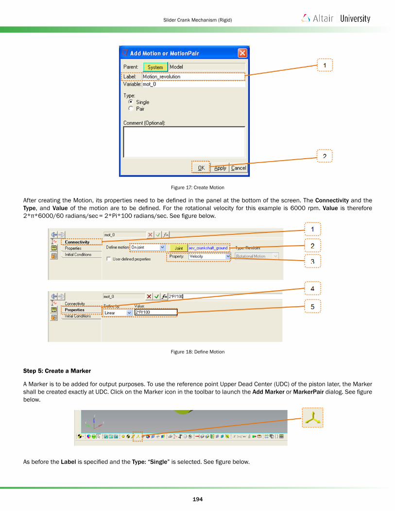
Figure 17: Create Motion

After creating the Motion, its properties need to be defined in the panel at the bottom of the screen. The Connectivity and the Type, and Value of the motion are to be defined. For the rotational velocity for this example is 6000 rpm. Value is therefore 2*π*6000/60 radians/sec = 2*Pi*100 radians/sec. See figure below.

Figure 18: Define Motion

Step 5: Create a Marker

A Marker is to be added for output purposes. To use the reference point Upper Dead Center (UDC) of the piston later, the Marker shall be created exactly at UDC. Click on the Marker icon in the toolbar to launch the Add Marker or MarkerPair dialog. See figure below.

As before the Label is specified and the Type: “Single” is selected. See figure below.

195


Figure19: Create Marker

To define the Marker further, as Parent, the piston should be chosen and as an Origin the point “UDC_piston”, which was created before, shall be used. You have additional options to specify the orientation of the Marker.

Figure 20: Define Marker

Step 6: Create Outputs

In this step the outputs, which should be evaluated, shall be created and defined using the Marker that was created in Step 5. We are interested in the displacement, velocity and the acceleration of the piston as calculated in the coordinate system of Marker_UDC_piston. So we will create these outputs.

Click on the Output icon shown below.

196


This will cause the Add Output dialog to pop-up. As with all other entities, specify a descriptive name in the label field.

Figure 21: Create Output

Clicking OK creates the output and the Output panel shows up at the bottom of the screen.

Four attributes are to be specified for each output:

• The output type – valid types are displacement, velocity, acceleration and force

• The two bodies between which the output is desired

• The points on each body

• The coordinate system in which the results are calculated

The Output panel allows you specify these. See figure below.

Figure 22: Define Marker

197


“Piston_velocity” and “Piston_acceleration” shall be created with the same Bodies, Points on the Bodies and the Reference Marker. The only modification is the type of the output within the dropdown menu (Fig. 22, # 1) by using Velocity and Acceleration respectively.

Hint: As an alternative to the creation of three outputs, subsequent post-processing allows you to manually calculate the velocity and the acceleration by differentiation of the displacement outputs. With this approach only the output for the displacement is necessary.

Step 7: Set The Simulation Parameters

In this step the MotionSolve run file and the Simulation Parameters are defined. Click on the Run icon in the toolbar. The Run Panel is displayed at the bottom of the screen. See figure below.

Select the Main tab, and click on the Folder icon next to Save as.

This will launch the file dialog as shown below. Choose the correct folder to save your results, and click OK as shown below.

198


Figure 23: Set Simulation Parameters

Finally specify the end time and print interval. We will choose a Print Interval of “0.0001s”. 100 output steps (0.01/0.0001) are generated in the simulation

Step 8: Check The Model

The model is now complete, and the next step is to check the model to make sure there are no errors. The model checker can be found in menu at Tools > Check Model. See figure below.

Selecting Check Model launches the Check Model window. MotionView will tell you some of the properties of the system you have defined. See figure below.

199


Figure 24: Check Model

Note: To see the Check Model summary as above you may first need to define the kind of model check to be pursued. Go to: Tools > Options > Check Model to configure the check model

It can be shown that the system had 18 degrees of freedom at the beginning, 17 of which were removed by joints and one by the rotational motion. Hence, according to the Grübler equation (Chapter 1.2) and consistent with MotionView calculations, the system has zero degrees of freedom. You have just created a kinematic model.

If one discovers that the sum of the DOF is negative during the model check, the chosen joints will have to be checked again and to be modified. A negative count for DOF implies that some of the constraints are redundant. MotionSolve will release the necessary constraints to obtain a determinate system. However, this may not be what you want.

Solver Run

The model is now ready for simulation. Click Run in the run panel. See figure below.

The solver run is initiated and the Solver window, shown below, appears. All Solver output is seen in real time in this window. Do not worry if the data scrolls by too quickly. You can always look at the solver log file more leisurely, using the editor of your choice.

200


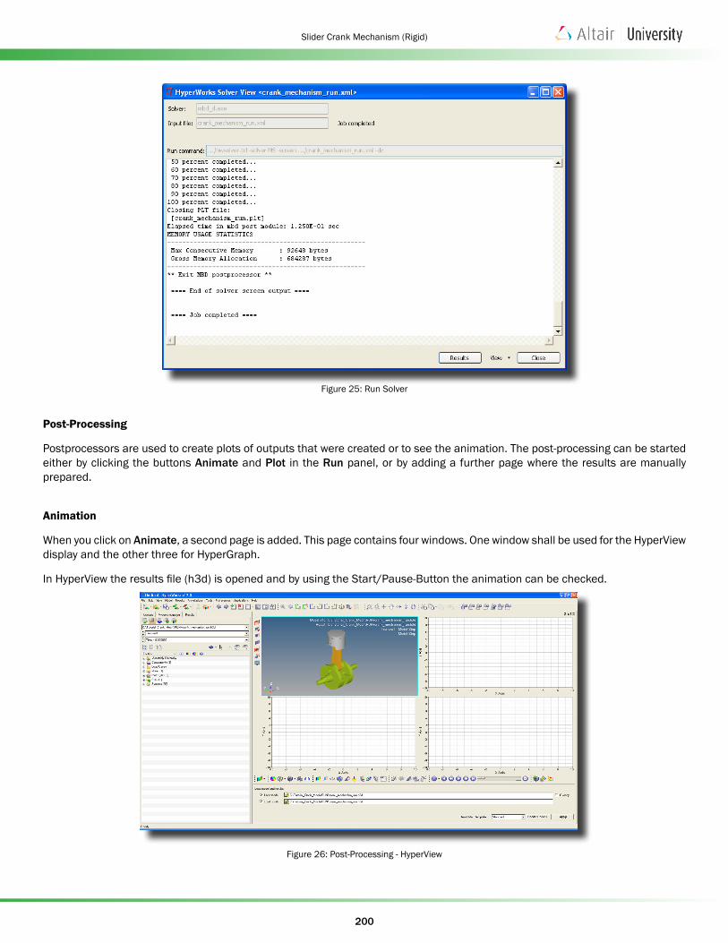
Figure 25: Run Solver

Post-Processing

Postprocessors are used to create plots of outputs that were created or to see the animation. The post-processing can be started either by clicking the buttons Animate and Plot in the Run panel, or by adding a further page where the results are manually prepared.

Animation

When you click on Animate, a second page is added. This page contains four windows. One window shall be used for the HyperView display and the other three for HyperGraph.

In HyperView the results file (h3d) is opened and by using the Start/Pause-Button the animation can be checked.

Figure 26: Post-Processing - HyperView

201


Plotting

Results may be plotted in HyperGraph. The HyperGraph windows can plot the displacement, velocity and acceleration outputs versus the rotation angle, Phi [deg].

One possible way to prepare the results in HyperGraph is shown below. This is a two-step process.

• Click on the Define Curves toolbar

• Click on the Add button to add curves

• Specify the X axis of the plot: abf-result file Time

• Specify the Y axis of the plot: Select Math radio button and define y = x

Figure 27a: Post-Processing – HyperGraph Define Curves Panel

• Now turn off Curve 1 in the Plot Manager. Create a second curve, Curve2 as shown below.

• Specify the X axis of the plot: Math = [Y-value of Curve 1]*36000

• Specify the Y axis of the plot: abf-result DZ_piston_displacement_with_respect_to_ground

Figure 27b: Post-Processing – HyperGraph Define Curves Panel

Now change the Axis Scale (0 to 360) and Text adjust manually (Figure 28)

Figure 28: Post-Processing – HyperGraph Set Axis

202


You can follow the same process for plotting velocity and acceleration results. Once all the plots are inserted, your screen should look like the screen shot below.

Figure 29: Post-Processing – Results

Validation

Piston distance to upper dead center (UDC)

203


The detailed calculation (editable) is in the Excel sheet below.

Figure 30: Validation – Excel Calculation

Figure 31: Validation – Analytical (Left) Vs. MBD-Simulation (right)

204


Hint: If one wants to get into the process in any position and load an existing model, then it is possible because of user-based file movements that the graphic output file cannot be found. Thus the bodies have to be assigned manually to this file again.

This procedure shall be shown for the crank-shaft model.

Figure 32: Load Model – Graphics Missing

Clicking on Graphics > Crankshaft shows, that the Graphical source is missing. Then one should reference as in Figure 33 shown the needed graphic for every single body by using the defined Output Graphic File.

Figure 33: Re-Organizing Graphical Source

8 Tutorial: The Slider Crank Mechanism - UPV Crank Mechanism.pdf · After clicking OK the geometry...

Documents

Transcript of 8 Tutorial: The Slider Crank Mechanism - UPV Crank Mechanism.pdf · After clicking OK the geometry...