7000514 IEEE JOURNAL OF SELECTED TOPICS IN QUANTUM ELECTRONICS, VOL. 20, NO. 2, MARCH/APRIL 2014

Modeling Light Scattering in Tissue as ContinuousRandom Media Using a Versatile Refractive

Index Correlation FunctionJeremy D. Rogers, Andrew J. Radosevich, Ji Yi, and Vadim Backman

(Invited Paper)

Abstract—Optical interactions with biological tissue providepowerful tools for study, diagnosis, and treatment of disease. Whenoptical methods are used in applications involving tissue, scatteringof light is an important phenomenon. In imaging modalities, scat-tering provides contrast, but also limits imaging depth, so modelshelp optimize an imaging technique. Scattering can also be usedto collect information about the tissue itself providing diagnos-tic value. Therapies involving focused beams require scatteringmodels to assess dose distribution. In all cases, models of lightscattering in tissue are crucial to correctly interpreting the mea-sured signal. Here, we review a versatile model of light scatteringthat uses the Whittle–Matern correlation family to describe the re-fractive index correlation function Bn(rd). In weakly scatteringmedia such as tissue, Bn(rd) determines the shape of the powerspectral density from which all other scattering characteristics arederived. This model encompasses many forms such as mass fractaland the Henyey–Greenstein function as special cases. We discussnormalization and calculation of optical properties including thescattering coefficient and anisotropy factor. Experimental methodsusing the model are also described to quantify tissue properties thatdepend on length scales of only a few tens of nanometers.

Index Terms—Biophotonics, continuous random media, massfractal, scattering, tissue optics.

I. INTRODUCTION

IN BIOLOGY and medicine, optical techniques enable non-invasive measurements of living tissue. Microscopy is par-

ticularly ubiquitous because it enables visualization of individ-ual cells and even organelles. There is a continuous effort toresolve ever finer detail to assess the most fundamental proper-ties of living organisms. However, resolution in optical imaging

Manuscript received June 19, 2013; revised August 8, 2013; accepted Au-gust 26, 2013. Date of publication September 6, 2013; date of current versionOctober 25, 2013. This work was supported by the National Institutes of Healthunder Grant R01CA128641, Grant R01CA155284, and Grant R01EB003682,and the National Science Foundation under Grant CBET-1240416. The workof A. J. Radosevich was supported by a National Science Foundation GraduateResearch Fellowship under Grant DGE-0824162.

J. D. Rogers is with the Department of Biomedical Engineering, Universityof Wisconsin, Madison, WI 53706 USA (e-mail: jdrogers5@wisc.edu).

A. J. Radosevich, J. Yi, and V. Backman are with the Department ofBiomedical Engineering, Northwestern University, Evanston, IL 60208 USA(e-mail: andrewradosevich2014@u.northwestern.edu; ji-yi@u.northwestern.edu; v-backman@northwestern.edu).

Color versions of one or more of the figures in this paper are available onlineat http://ieeexplore.ieee.org.

Digital Object Identifier 10.1109/JSTQE.2013.2280999

systems poses a challenge to studying length scales less thanthe diffraction limit (about half the wavelength). Some veryclever techniques have been developed to sidestep this issue,including STED, STORM, and other super resolution meth-ods [1]. These methods enable imaging or reconstruction ofextraordinary detail, but typically require contrast agents andcareful tissue preparation. Therefore, a niche remains availablefor additional methods of quantifying fine length scales. Sev-eral methods with potential to fill that niche rely on analysis ofscattering.

Many applications are critically affected by light scatteringin tissue. Sometimes scattering is considered a nuisance, andresearch has been devoted to optical clearing of tissue [2]. Atthe same time, in many imaging techniques, scattering providesthe image contrast, for example, in confocal microscopy or op-tical coherence tomography (OCT). Diffuse optical tomogra-phy is perhaps the best example of using measurement of lightpropagation in tissue to reconstruct tissue features that cannototherwise be imaged and relies on reconstructing tissue prop-erties based on transport theory due to multiple scattering [3].Models of scattering are also important in treatment methodssuch as photodynamic therapy where carefully controlling thedistribution of energy is crucial for successful treatment [4].

Clearly, methods of modeling radiative transport in tissue areneeded for a wide range of applications including treatment ortherapy, imaging, and characterization or diagnosis. One of themost widely used modeling methods is to numerically solve theradiative transport equation using Monte Carlo (MC) simula-tions. MC works by simulating a large number of rays as theypropagate by sampling two probability distribution functions:1) The path length traveled between scattering events is de-scribed by a decaying exponential associated with mean freepath (Beer–Lambert law). 2) The angular distribution of scat-tered light for a single scattering event is called the phase func-tion. The shape of the phase function is highly dependent on thescattering model. While MC is a powerful simulation method,the results are only as good as the model it is based on.

In this paper, we describe the use of a particularly flexiblechoice for modeling tissue scattering. The model assumes thattissue can be described as a continuous random media ratherthan discrete particles, which agrees with observations of ma-terial distribution such as electron microscopy. The model isbased on the Whittle–Matern (WM) correlation family and ishighly flexible, encompassing several other models previously

1077-260X © 2013 IEEE. Personal use is permitted, but republication/redistribution requires IEEE permission.See http://www.ieee.org/publications standards/publications/rights/index.html for more information.

ROGERS et al.: MODELING LIGHT SCATTERING IN TISSUE AS CONTINUOUS RANDOM MEDIA 7000514

used to describe tissue including mass fractals and the Henyey–Greenstein (HG) phase function. While direct measurements ofthe refractive index correlation function would provide the bestmodel of tissue, such measurements are currently not possiblewith the necessary resolution of a few tens of nanometers. In themeantime, the WM provides a good alternative. We summarizethe choices to make within this model and show how opticalproperties are calculated. Finally, we demonstrate several tech-niques where this model provides both excellent agreement withdata and also a means to quantify the distribution of length scaleswell below the diffraction-limited resolution.

II. TISSUE, STRUCTURE, AND REFRACTIVE INDEX

Tissue is made up of many interconnected, arbitrarily shapedstructures that span a wide range of length scales. Many textscan provide an overview of the components of cells or tissue [5].For example, the extracellular matrix (ECM) is composed pri-marily of collagen and elastin fibers ranging in size from 10to 500 nm in diameter. Cells themselves are of various shapesand sizes on the order of tens of micrometers. Cells are in turncomprised of smaller structures such as membranes (10 nm)and organelles including the nucleus (5–10 μm), mitochondria(0.2–2 μm), and many others. Cells also contain a cytoskeletonmade of filaments from 7 to 25 nm in diameter. The nucleus con-tains nucleoli (0.5–1.0 μm) and DNA in the form of chromatin.The organization of chromatin is the subject of active research,but electron microscopy reveals that chromatin is found in theform of heterochromatin and euchromatin and appears to havedifferent densities. These form globules with length scales ofhundreds of nanometers.

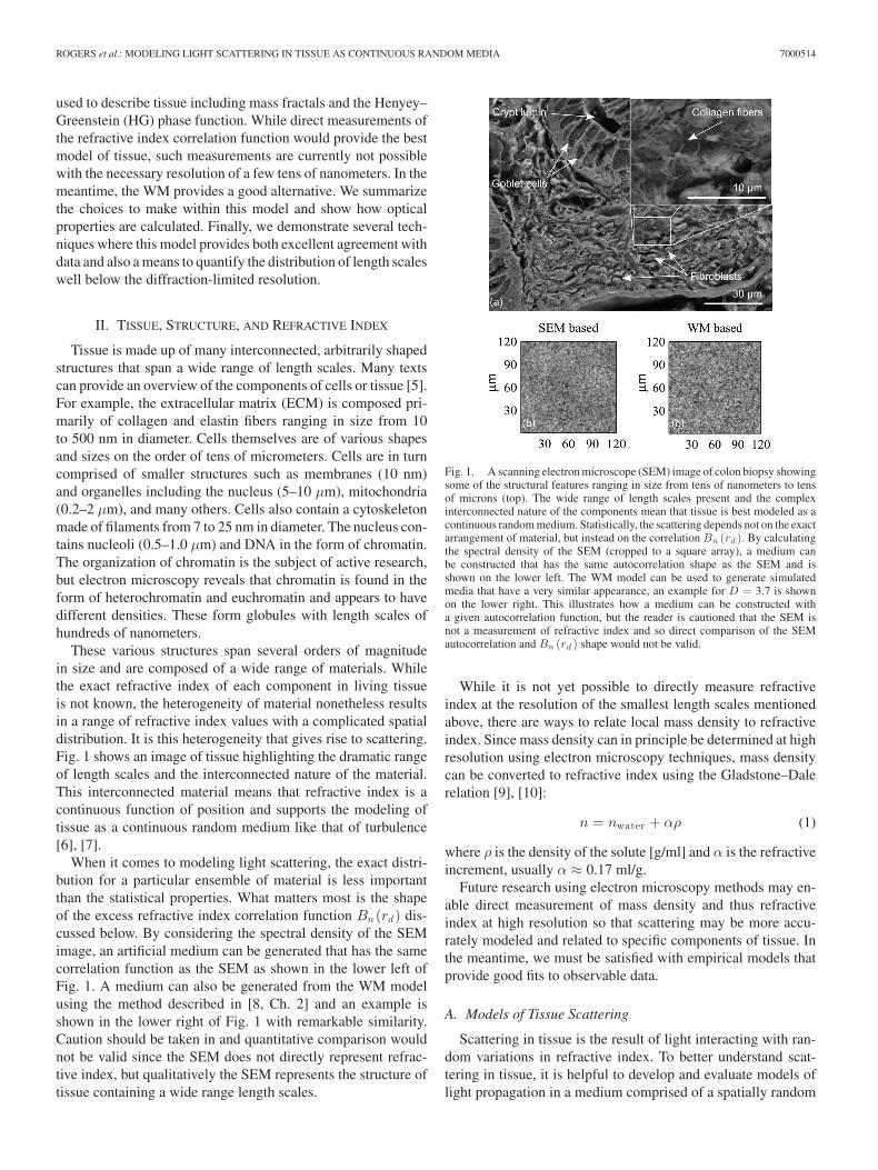
These various structures span several orders of magnitudein size and are composed of a wide range of materials. Whilethe exact refractive index of each component in living tissueis not known, the heterogeneity of material nonetheless resultsin a range of refractive index values with a complicated spatialdistribution. It is this heterogeneity that gives rise to scattering.Fig. 1 shows an image of tissue highlighting the dramatic rangeof length scales and the interconnected nature of the material.This interconnected material means that refractive index is acontinuous function of position and supports the modeling oftissue as a continuous random medium like that of turbulence[6], [7].

When it comes to modeling light scattering, the exact distri-bution for a particular ensemble of material is less importantthan the statistical properties. What matters most is the shapeof the excess refractive index correlation function Bn (rd) dis-cussed below. By considering the spectral density of the SEMimage, an artificial medium can be generated that has the samecorrelation function as the SEM as shown in the lower left ofFig. 1. A medium can also be generated from the WM modelusing the method described in [8, Ch. 2] and an example isshown in the lower right of Fig. 1 with remarkable similarity.Caution should be taken in and quantitative comparison wouldnot be valid since the SEM does not directly represent refrac-tive index, but qualitatively the SEM represents the structure oftissue containing a wide range length scales.

Fig. 1. A scanning electron microscope (SEM) image of colon biopsy showingsome of the structural features ranging in size from tens of nanometers to tensof microns (top). The wide range of length scales present and the complexinterconnected nature of the components mean that tissue is best modeled as acontinuous random medium. Statistically, the scattering depends not on the exactarrangement of material, but instead on the correlation Bn (rd ). By calculatingthe spectral density of the SEM (cropped to a square array), a medium canbe constructed that has the same autocorrelation shape as the SEM and isshown on the lower left. The WM model can be used to generate simulatedmedia that have a very similar appearance, an example for D = 3.7 is shownon the lower right. This illustrates how a medium can be constructed witha given autocorrelation function, but the reader is cautioned that the SEM isnot a measurement of refractive index and so direct comparison of the SEMautocorrelation and Bn (rd ) shape would not be valid.

While it is not yet possible to directly measure refractiveindex at the resolution of the smallest length scales mentionedabove, there are ways to relate local mass density to refractiveindex. Since mass density can in principle be determined at highresolution using electron microscopy techniques, mass densitycan be converted to refractive index using the Gladstone–Dalerelation [9], [10]:

n = nwater + αρ (1)

where ρ is the density of the solute [g/ml] and α is the refractiveincrement, usually α ≈ 0.17 ml/g.

Future research using electron microscopy methods may en-able direct measurement of mass density and thus refractiveindex at high resolution so that scattering may be more accu-rately modeled and related to specific components of tissue. Inthe meantime, we must be satisfied with empirical models thatprovide good fits to observable data.

A. Models of Tissue Scattering

Scattering in tissue is the result of light interacting with ran-dom variations in refractive index. To better understand scat-tering in tissue, it is helpful to develop and evaluate models oflight propagation in a medium comprised of a spatially random

7000514 IEEE JOURNAL OF SELECTED TOPICS IN QUANTUM ELECTRONICS, VOL. 20, NO. 2, MARCH/APRIL 2014

distributions of refractive index. This distribution could be inthe form of a continuous function of refractive index (like at-mospheric turbulance) or in the form of discrete particles. Manymodels of tissue scattering approximate tissue as a collection ofrandomly placed spheres or spheroids [11]–[13]. This is plau-sible considering that organelles such as nuclei, mitochondria,lysosomes, vacuoles, and even whole cells are approximatelyspherical (or spheroidal) in shape. The scattering from such iso-lated particles can be analytically described by the Mie solutionto scattering from spheres [14], [15]. Scattering from a randommedium made up of many such spheres (i.e., a cloud of rain-drops) is calculated by then incoherently summing the scatteringfrom many spheres according to the number density. However,in many cases, it is hard to argue that the shape is spherical soMie theory is inherently limited.

Another ubiquitous model of tissue scattering is basedon the empirical observation that tissue scattering is usuallyanisotropic. That is, a very small volume of tissue scatters morelight in the forward direction at small angles than in the back-ward direction. A simple model of such anisotropic scatteringwas developed by Henyey and Greenstein to describe scatteringof interstellar dust and is now referred to as the HG phase func-tion [16]. Counterintuitively, the phase function has little to dowith the phase of a scattered ray. Instead, the term is historicaland refers to the apparent brightness of celestial bodies such asthe moon or planets as they pass through their phases. The func-tion is a normalized intensity as a function of the angle betweenincident and scattered direction.

Observing tissue scattering using methods such as goniome-ter and integrating sphere, Jacques et al. found the HG functionprovided a good model to match their observations [17]. It hassince become one of the most common models of tissue scat-tering. However, this model is limited in that it does not includethe dipole factor (discussed in Section IV-A) that leads to anonmonotonically decreasing function of angle that is typicallyobserved in scattering [11], [18] and it does not provide a phys-ical connection to the structures which generated it.

Other models of tissue scattering have been put forth and usedwith success and include delta-Eddington proposed by Josephet al. [19] and discussed in detail by Prahl [20] that uses thesum of a Dirac-δ function and cos θ dependence to describe thephase function, and the P3-approximation [21] that takes thefirst three terms in an expansion of the solution to the radiativetransport equation.

In choosing a model for tissue scattering, it is a good idea touse the simplest model that matches the experimental methodemployed to avoid over fitting. For example, when using an in-tegrating sphere and the inverse adding doubling (IAD) method[20], the experimental data are well modeled by the HG func-tion. However, as experimental methods evolve, some measure-ments cannot be explained with such a simple model, and it isnecessary to invoke a more complex model of scattering.

B. As New Methods Emerge, Better Models Are Needed

One challenge facing those wishing to model tissue scatteringis determining what model to use. Any model of scattering will

Fig. 2. Example of experimental data that cannot be explained using the HGfunction. Radiative transport in rat lung tissue is measured with EBS to producea probability distribution P (rs ) of the entrance/exit separation of rays scatteredin the tissue and eventually exiting. Two best fit models of P (rs ) computednumerically using MC are also shown based on WM (blue solid) and the specialcase of D = 3 which is equivalent to the HG phase function commonly used tomodel tissue. Fitting with a two parameter HG function produces a poor fit tothe small rs , while a three-parameter WM-based model results in an excellentfit to the experimental.

inherently contain approximations. Choosing the right model isall about choosing the most appropriate set of approximations.

Fig. 2 shows an example where a simple model of scatteringbased on the HG function is not sufficient to explain the exper-imental data. In these data, radiative transport is measured withenhanced backscattering (EBS) at length scales ranging frommuch less than the transport mean free path l′s to much greaterthan l′s , which for this tissue is about 200 μm. EBS measuresthe probability distribution P (rs) of ray exit distances relativeto the point of entry in a scattering medium, in other words thespatial impulse response of diffuse reflectance [22].

Most methods that measure radiative transport via backscat-tering are only sensitive to separations larger than l′s where thepropagation of light can be accurately modeled using the dif-fusion approximation [23]. The figure shows that the differentmodels tend to converge at these larger length scales, whilesmall distances exhibit more significant differences because inthis region, P (rs) is dominated by low order scattering and is,therefore, more sensitive to the shape of the phase function. Themodel curves are calculated by using the scattering model in MCsimulations of scattering to build a catalog of curves for rangesof parameters. Fits to experimental data are obtained by inter-polating the model simulation space to produce a lookup table.The dashed red line corresponds to the best fit obtained usingthe HG phase function, while a much better fit is obtained usingthe WM model with D = 3.75 highlighting the need for morea more advanced model for measurement methods that are ca-pable of discriminating between different correlation functionalforms.

III. RAYLEIGH–GANS–DEBYE APPROXIMATION

One of the most useful approximations that can be made inscattering from biological tissue is that of “weak” scattering. Inthis approximation, it is assumed that the scattered field is muchless significant than the incident field. This approximation is

ROGERS et al.: MODELING LIGHT SCATTERING IN TISSUE AS CONTINUOUS RANDOM MEDIA 7000514

also known as Rayleigh–Gans–Debye (RGD) scattering, the firstBorn approximation, or single scattering approximation. Here,we will use “RGD scattering” for brevity. This approximationcan be used to describe discrete particles as well as continuousmedia and has been extensively investigated by Ishimaru forother refractive index correlation functions, so we will followhis derivation for continuous random media [24]. Excellent dis-cussions of RGD scattering in particles are provided by Hulstand van de Hulst [25] as well as Bohren and Huffman [15].

A brief conceptual summary of the RGD approximation isas follows: When a plane wave traveling in free space passesthrough a particle, the dipoles that make up the particle are ex-cited and begin to oscillate reradiating electromagnetic energyaccording to the Rayleigh or dipole radiation pattern [26]. Inthe RGD approximation, the scattered field is insignificant rel-ative to the incident field, so secondary scattering events can beignored. This is equivalent to saying that the electric field arriv-ing at any point inside the particle is approximately the sameas the incident field. In other words, there is no phase delay orrefraction inside the particle. The phase of each dipole is thendetermined by its position along the z-axis (direction of incidentwave). The total effect of all the dipoles can then be treatedby coherently summing the field from each dipole to obtain thescattering amplitude function f(θ, φ). This summation can bemathematically written as an integral of relative excess refrac-tive index as a function of position nΔ(�r) = (n(�r) − 〈n〉)/〈n〉,where 〈n〉 is the expected value or average refractive index.The spherical wave can be written as a complex exponentialso that the operation takes the form of a Fourier transform. Weare typically interested in the intensity of scattering, since thisis the observable quantity. The intensity is proportional to thesquare of the amplitude scattering function, which is the Fouriertransform of nΔ(r). By applying the Wiener–Khinchin theorem,we see that the scattered intensity per unit volume as a func-tion of angle (known as the differential scattering cross sectionσ(θ, φ)) is proportional to the spectral density Φs(ks), whichis the Fourier transform of the autocorrelation of the excessrefractive index Bn (rd):

Φs(�ks) =1

(2π)3

∫∫∫Bn (�rd)e−i �ks · �rd d�rd (2)

where �rd is a displacement vector between any two points inthe medium. When the medium is statistically isotropic, Bn (�rd)is radially symmetric and can be represented as a 1-D functionof scalar displacement rd . The result simplifies to the productof a dipole factor 1 − sin2(θ) cos2(φ) multiplied by the spec-tral density evaluated at ks = 2〈n〉k sin(θ/2), where k is thefreespace wavenumber:

σ(θ, φ) = 2π(〈n〉k)4 (1 − sin2(θ) cos2(φ)

)Φs(ks)

= 2π(〈n〉k)4 (1 − sin2(θ) cos2(φ)

)1

(2π)3

∫ ∞

0Bn (rd)

4π sin (2〈n〉k sin(θ/2)rd)2〈n〉k sin(θ/2)

rddrd. (3)

Note that this relation works for a suspension of particlesas well as continuous media. For particles, the weak scatteringapproximation is valid when | n

〈n〉 − 1| � 1 and 2ka| n〈n〉 − 1| �

1, where a is the particle radius. That is to say, the excessrefractive index must be small and the phase delay as the wavetraverses the particle must be much less than the wavelength.

It is important to note that while the RGD scattering approx-imation is often referred to as the single scattering approxima-tion, this does not mean that it cannot be used to model largevolumes such as clouds or tissue where multiple scattering takesplace. What is required in the case of a particle is that single scat-tering is valid for a single particle. When a medium is composedof many such particles, light transport can be very accuratelycomputed numerically by methods such as MC [27]. The key isto accurately compute the angular probability for each scatter-ing event and then propagate rays according to mean free pathwith subsequent scattering events. Interestingly, the same is truefor continuous media.

The RGD approximation should, therefore, not be used tomodel an entire region of tissue, but rather to statistically modela representative volume just large enough to cause one scatter-ing event. Multiple scattering can then be treated as decoupledevents that can be summed according to the mean free pathand scattering function using computational methods like MC.Such simulations can be made even more accurate by using theExtended Huygens–Fresnel principle to account for the propa-gation of coherence in the case of multiple scattering, and anexcellent review of such treatment developed by Anderson andThrane is provided in [28, Ch. 17].

A. Validity of the RGD Approximation for Continuous Media

Unlike a particle, there is no clear boundary in continuousmedia over which the concept of single scattering can be ap-plied. Instead, in continuous media, the single scattering ap-proximation must be valid for a representative small volume ofmaterial. By representative, we mean that the volume must belarge enough to represent statistical ensemble of the medium,but small enough that single scattering approximation holds. Aslong as the volume can be defined for which small changes in thevolume result in the same differential scattering cross section perunit volume, the RGD approximation is valid. One could alsosay that ls > Ln must be true, where ls is the mean free path andLn is the outer length scale of the correlation beyond which themedium is not significantly correlated. In other words, a wave ofpropagating light must, on average, pass through enough mediato be statistically representative before being scattered. This wasrigorously investigated using finite-difference time domain andthe validity criterion can be written as σ2

n (〈n〉kLn )2 � 1 [29].

B. An Illustrative Example: Suspension of Spheres

While we are most interested in modeling continuous mediain this paper, it is instructive to follow through an example usinga suspension of spheres. We can then compare the resultingscattering functions to those obtained with the Mie solution.Incidentally, it is just such media in the form of polystyrenemicrosphere suspensions that are often used as tissue phantomsin research labs.

To begin, we must consider Bn (rd) for a suspension ofspheres. For a sphere of radius a, the autocorrelation function

7000514 IEEE JOURNAL OF SELECTED TOPICS IN QUANTUM ELECTRONICS, VOL. 20, NO. 2, MARCH/APRIL 2014

Fig. 3. Comparison of the Mie solution for a suspension of microspheres to σ(θ, φ) calculated using the RGD approximation. The top two panels show thecalculation for polystyrene microspheres in water and while the 100 nm diameter spheres (upper left) show good agreement, the approximation breaks down for400 nm spheres (upper right). However, when the index contrast is low n1/n0 = 1.02 as in the bottom row, the agreement holds for 400 nm spheres (lower left)and even for large spheres of 3.0 μm (lower right). Calculations used a wavelength of 500 nm.

can be computed analytically, so Bn (rd) is simply scaled by thevariance of the refractive index:

B(sphere)n (rd) =

⎧⎨⎩

σ2n

(2a − rd)2(4a + rd)16a3 , where rd ≤ a

0, where rd > a.(4)

We must next calculate the expected value of refractive index〈n〉 and the variance σ2

n of the relative excess refractive indexnΔ = n/〈n〉 − 1. These values depend on the refractive indexof the spheres ns , surrounding medium nm , and the volumefraction Cv occupied by spheres

〈n〉 = Cvns + (1 − Cv )nm (5)

σ2n = Cv

(ns

〈n〉 − 1)2

+ (1 − Cv )(

nm

〈n〉 − 1)2

. (6)

The Fourier transform of this function can be calculated ana-lytically

Φs(ks) =3(1 − Cv )Cv (nm − ns)2

2π2(Cvnm − nm − Cvns)2a3k6s

× (ksa cos(ksa) − sin(ksa))2 (7)

and substituted into (3) to calculate the differential scatteringcross section. If we plot the results and compare to the Miesolutions as in Fig. 3, we can see excellent agreement for verysmall particles (top left) or very small refractive index contrast(bottom left). The accuracy begins to decrease as particle size

increases a little (top right). For weaker refractive index contrast,the particle size can get much larger before the agreement breaksdown (bottom row). This is consistent with the requirements ofthe single scattering approximation described in Section III-A.

IV. QUANTIFYING STRUCTURE WITH A REFRACTIVE

INDEX CORRELATION FUNCTION

Scattering from a medium can be computed analytically ornumerically for a known distribution of dipoles or, equivalently,a known distribution of refractive index. This is rarely if ever thecase for biological tissue. It is, therefore, of interest to determinestatistical average scattering from a random medium where theexact distribution of index is unknown, but the statistical prop-erties are known, or can be approximated. One way to describethe average scattering properties of a random medium is to de-scribe the average shape of differential scattering cross sectionfrom a small representative volume of material. As seen in Sec-tion III, an expected value of the differential scattering crosssection σ(θ, φ) can be directly calculated from the refractiveindex correlation function Bn (rd).

A. WM Correlation Family

The best model of tissue scattering would be based on a di-rect measurement of refractive index correlation over the entirerange of lengths scales to which scattering is sensitive. This iscurrently not possible, and so lacking a catalog of refractive

ROGERS et al.: MODELING LIGHT SCATTERING IN TISSUE AS CONTINUOUS RANDOM MEDIA 7000514

Fig. 4. Examples of the WM function for different values of D normalizedsuch that Bn (rd = Ln ) = 1. Inset shows the same functions on a log–logscale.

index correlation functions in tissue, we can choose to modelthe correlation function using a functional form to approximatethe actual statistical correlation function.

Several correlation functions have been used to model con-tinuous random media. Chapter 16 in Ishimaru’s text describesexponential correlation that leads to the Booker–Gordon for-mula, the Gaussian model, and the Kolmogorov spectrum alsoknown as the von Karman spectrum which is based on a powerlaw with a specific power [24], [30]. A number of papers haveproposed a fractal model for tissue [6], [7]. Mass fractals arecharacterized by power law correlation functions where the massfractal dimension is related to the power. Interestingly, all ofthese models as well as the HG function can be described by theWM correlation family [30], which is the product of a powerlaw and a modified Bessel function of the second kind of order(D − 3)/2,

Bn (rd) = An

(rd

Ln

)(D−3)/2

KD −32

(rd

Ln). (8)

The fact that the WM family of correlation functions is soflexible and encompasses many other models makes it an attrac-tive choice. The parameter D controls the shape of function andcan be used to represent a wide range of plausible correlationsincluding:

1) Gaussian: D → ∞;2) exponential: D = 4;3) stretched exponential: 3 < D < 4;4) Kolmogorov/von Karman: D = 11/3;5) HG: D = 3;6) power law: D < 3.Examples of the functional form for several values of D are

shown in Fig. 4. Note that when D < 3, the medium can beconsidered a mass fractal and the parameter D takes on thespecial meaning of mass fractal dimension.

Fig. 5 shows an example of the differential scattering crosssection σ(θ, φ) (3) calculated for vertically polarized light andD = 3. For this case, the shape around the equator at σ(θ, φ =90◦) corresponding to the shape of the HG phase function.However, an important difference is the inclusion of the dipolefactor. When incident light is unpolarized, the phase function can

Fig. 5. An example of the differential scattering cross section σ(θ, φ) for leftto right propagating vertically polarized light. This example is computed usingthe WM function discussed below with parameter D = 3 in which case theshape around the equator (φ = 90◦) corresponds to the HG phase function. Thedipole factor produces the dimples oriented in the plane of the electric fieldpolarization.

be calculated by averaging over φ resulting in a phase functionwith a minimum at θ = 90◦ [31]. This extension of the HGphase function more accurately reflects physical measurements.For example, Mourant reported goniometer measurements oftissue along with fitting of the HG function, but the HG phasefunction could not match the measurements in the backscatteringdirection [11], [18].

B. Normalization

The WM correlation family is useful because it can takeon so many different functional forms. This does, however,create some challenges in terms of normalizing the function. Theconvention typically used in signal processing is that correlationfunctions are normalized such that the value at the origin (rd =0) is equal to 1, while in statistical disciplines, it is equal to thevariance—in our case, the variance of excess refractive indexσ2

n . However, since power laws are unbounded at the origin, thisconvention is impossible to implement for D < 3. Therefore,no single normalization can be used to satisfy convention in thebounded case D > 3 and the unbounded case D < 3.

The WM function has three parameters: D, An , and Ln . Theshape is determined by D, while the latter two can be thoughtof as scaling parameters. Ln scales the horizontal axis, whileAn scales the vertical axis. Ln also represents a transition pointbeyond which the function decays as an exponential. There areseveral options for the normalization coefficient An , and eachhas advantages and disadvantages.

It should be noted that these normalization options only af-fect the interpretation of the coefficient σ2

n as the variance ofrefractive index. The function Bn (rd) is not arbitrary and ac-tually represents a physical function that could, in principle, bephysically measured. In media where the best fit of Bn (rd) isfor D ≤ 3, the actual physical value of σ2

n is still finite, but thepower law only extends down to some small length scale belowwhich the shape is irrelevant. This is sometimes called the innerscale of turbulence. When this inner scale is much smaller thanthe wavelength, the error in Φs between the unbounded modelfunction and the actual refractive index correlation function issmall [31]. Nevertheless, it is useful to explore several optionsfor normalizing Bn (rd).

7000514 IEEE JOURNAL OF SELECTED TOPICS IN QUANTUM ELECTRONICS, VOL. 20, NO. 2, MARCH/APRIL 2014

1) Whittle and Matern Normalization: Bn (0) = 1 for D >3: A brief description of the history of the WM function andsome closely related functions used in modeling atmosphericturbulence is provided by Guttorp and Gneiting [30]. Theseauthors describe the normalization that Whittle and Matern used.In this case, the function is normalized to 1 (or σ2

n ) at rs = 0for values of D > 3 that result in a bounded function. In otherwords, σ2

n is the variance for D > 3, and just a parameter forD < 3:

An = σ2n

25−D

2

|Γ(D−32 )|

for D > 3. (9)

The advantage of this normalization is that it is normalizedat the origin when it is bounded, as any actual correlation func-tion should be. The disadvantage is that as D gets smaller andapproaches 3, the narrow shape of the function forces the magni-tude to zero at any finite value of rd . This, in turn, results in thetotal scattering cross section collapsing to zero. Additionally,the function is identically zero for D = 3, and so we lose theability to model the HG function. Guttorp and Gneiting arguethat (D − 3)/2 must be greater than 0 for this correlation to bevalid (eliminating the need for the absolute value of the gammafunction). This is true in that σ2

n cannot be defined when D ≤ 3,but many interesting cases occur for these values of D, includ-ing a power law corresponding to mass fractals. When D ≤ 3,the function Bn (rd) approaches a power law for small rd andso is infinite at the origin.

2) Normalized at a Minimum Length Scale: Bn (rmin) = σ2n :

One possible normalization is to attempt to mimic reality. WhenD < 3, Bn (rd) approximates a power law corresponding to amass fractal organization of material. In nature, fractals occurthat exhibit self-similarity over a range of scales and, therefore,are described by a power law correlation function. However, therange of scales over which the true function closely follows apower law is not infinite. For example, in tissue, one may observelength scales corresponding to the size of a cell. Zooming in,one observes a similar organization in organelles, but at a lengthscale an order of magnitude smaller. Zooming in yet further, onemight observe globule organization of macromolecules. Thisapproximate self-similarity over several magnitudes of lengthscales is what gives rise to a power law correlation function.However, this power law cannot extend to infinitely small lengthscales. At some small scale, only molecules are left and the verydefinition of refractive index becomes difficult to interpret. Ifthe actual correlation function were known, the mode could befit by defining a minimum length scale rmin and normalize thefunction at this value:

An = σ2n

(rmin

Ln

)(3−D )/2 /KD −3

2

(rmin

Ln

). (10)

Provided that rmin is chosen correctly, the value of the modelfunction at rmin can be close to the true value σ2

n . The advantageof this normalization is that there is an intuitively satisfyingnotion that the correlation always starts at σ2

n for some arbitrarilysmall value regardless of the value of D. One problem with thisnormalization is that it introduces a fourth parameter rmin thatmust be arbitrarily chosen. Since rmin is arbitrary, the value of

σ2n is also arbitrary which makes interpretation of σ2

n difficultsince it is no longer a material property but depends on thechosen rmin . For a power law, a small change in the chosenvalue of rmin could result in a large change in the model’svalue of σ2

n and it does not necessarily correspond to the actualvariance of the real medium.

3) Normalized to Value c at rd = Ln : Since the previousnormalization can lead to a misinterpretation of the meaning ofσ2

n , one alternative is to simply normalize the model at a finitevalue of rd that is already defined in the model, namely Ln .The normalization constant c is not interpreted as variance ofrefractive index; it is simply the value that scales the model tomatch the actual medium:

An =c

KD −32

(1). (11)

This normalization has the advantage that the it is well behavedfor all values of D. Of course, the function is infinite at rd = 0for value of D ≤ 3 as expected. When D > 3, the function isindeterminate at rd = 0, but the limit is bounded, so this posesno problem for modeling scattering. The disadvantage is thatrelating this scaling parameter to σ2

n requires an extra step, butthis can be easily dealt for values of D > 3:

c = σ2n

25−D

2

Γ(

D−32

)KD −32

(1). (12)

When D ≤ 3, σ2n could be determined for the actual medium,

but is not explicitly part of the model.These first three choices do not depend on scattering: they

simply describe the properties of a medium. There are, how-ever, a few additional options for normalization that amountto normalizing the spectral density independent of the scale ofBn (rd). These retain the dependence on the shape of Bn (rd),but not the magnitude.

4) Normalized Spectral Density:∫ ∞

0 Φs(ks)dks = 1: An-other option is to normalize the spectral density Φs such that∫ ∞

0 Φs(ks)dks = 1. In this case, the function takes the form ofa Pearson distribution type VII:

An =2π

L2n (D − 3)

25−D

2

Γ(D−32 )

. (13)

The advantage is that the spectral density is never unboundedfor any value of D. One disadvantage is that because Φs isa probability function, it has no dependence on the varianceof refractive index σ2

n . This choice of normalization requiresD > 1 and has zeros, singularities, or is indeterminate at rd = 0for values of D = 2, 3, 4.

5) Rayleigh Scattering Normalized:

An =σ2

n

√2/π

2(D/2−2)Γ(D/2). (14)

Another option is to normalize such that the scattering coef-ficient μs converges to the same value for any value of D inthe Rayleigh limit where Ln � λ. This is appealing in that asthe correlation function becomes much smaller than the wave-length, there should not be any dependence of the shape of

ROGERS et al.: MODELING LIGHT SCATTERING IN TISSUE AS CONTINUOUS RANDOM MEDIA 7000514

the correlation function (or particle). This normalization is thenequivalent to saying that all small particles look the same tolong waves and scattering depends only on the mean free pathindependently of the shape of the correlation function. The dis-advantage is that the scattering coefficient is indeterminate forvalues of D = 2, 4.

V. CALCULATING OPTICAL PROPERTIES FROM DIFFERENTIAL

SCATTERING CROSS SECTION

Armed with a method to calculate the differential scatter-ing cross section per unit volume σ(θ, φ), we can calculatethe optical parameters typically used to characterize a scatter-ing medium. These parameters include the scattering coefficientμs = 1/ls which is the inverse of mean free path ls . The scatter-ing coefficient is equal to the total scattering cross section perunit volume and is easily obtained by integrating,

μs =∫ 2π

φ=0

∫ π

θ=0σ(θ, φ) sin θdθdφ. (15)

The anisotropy coefficient g = 〈cos θ〉 is the average of thecosine of the scattering angle,

g =

∫ 2π

φ=0

∫ π

θ=0 σ(θ, φ) cos θ sin θdθdφ∫ 2π

φ=0

∫ π

θ=0 σ(θ, φ) sin θdθdφ. (16)

Anisotropy determines the degree to which scattering is for-ward directed where g = 1 corresponds to completely forwardscattering, 0 < g < 1 corresponds to scattering that is forwarddirected, and g = 0 corresponds to isotropic scattering. Anotherparameter commonly used to describe media such as tissue thatare typically strongly forward scattering with values of g ≈ 0.9is the reduced scattering coefficient,

μ′s = μs (1 − g) . (17)

Also of interest is the backscattering coefficient,

μb = 4π · σ(θ = π). (18)

When the WM model is used, these relationships can be cal-culated analytically in terms of the model parameters. This wasshown by Sheppard [32] and later extended by Rogers et al. toinclude the effect of the dipole factor [31]. What is particularlyinteresting is the spectral relationship of the optical propertiesthat can be readily measured. For example, the spectral depen-dence of μ′

s(k) can be measured and then related to the modelparameter D. For example, in biological tissue, the fact that gis large indicates that the medium contains structure large com-pared to the wavelength, or kLn � 1. In this regime, μ′

s ∝ λD−4

for D < 4.

VI. EXPERIMENTAL METHODS FOR QUANTIFICATION

OF MODEL PARAMETERS

There are a number of experimental methods capable ofmeasuring scattering properties of tissue, for example, Go-niometer, integrating sphere (with the IAD method), Confocal,OCT/ISOCT, and P (rs)/EBS. Of these, the first two require sig-nificant tissue preparation to create a thin uniform slab of tissue

that is then measured in transmission and reflection. AlthoughHall et al. showed that thicker tissue samples can be used ifmultiple scatting is corrected using MC [33], prepared tissueis still required. The remaining methods are attractive becausethey can be used in reflection and so have potential to be usedin vivo. Jacques et al. recently demonstrated quantification ofproperties including μ′

s and anisotropy g using confocal andOCT methods [34]. As illustrated in Fig. 2, some methods suchas EBS are particularly sensitive to the shape of σ(θ, φ) and,therefore, enable measurement of parameter D.

While EBS measurement of P (rs) provides an excellentquantification of tissue properties and demonstrates the advan-tages of a more complex 3 parameter model, one limitation isthe assumption that the medium is statistically homogeneous.We know that tissue is often a layered medium, so methodscapable of quantifying the optical properties locally at differentpositions and depths would be of great utility. One such methodis based on OCT and allows assessment of properties in an imag-ing modality, a technique referred to as inverse spectroscopicOCT (ISOCT).

The unique advantage of ISOCT is that it is capable of imag-ing tissue structures in 3-D space, while simultaneously pro-viding complete quantification of the optical properties and (byassuming the WM model) the correlation functional form [35],[36]. The depth resolving capability in OCT is realized by inter-ferometry between the reference field and the sample scatteringfield. The primary contrast is the coherent elastic scattering fromthe tissue heterogeneity on which the WM scattering model ap-plies. In addition, OCT requires a broadband source to eliminatethe 2π ambiguity, providing an opportunity to analyze the scat-tering spectrum from a scattering medium such as tissue.

The signal in OCT can be approximated to be proportionalto the backscattering coefficient μb [see (18)]. Also the signaldecay along the penetration depth is exponential and scales withμs . Thus, the OCT image intensity can be modeled as [35]

I2(z) = rI20μb(z)4π

Le−μs ·2〈n〉z (19)

where I0 is the illumination intensity, r is the reflectance of thereference arm, L is the temporal coherence length of the source,z is the penetration depth, and the mean refractive index ofthe medium is 〈n〉 ≈ 1.38. Further, a short-time Fourier trans-form (STFT) can be performed to obtain the spatially resolvedspectra, and thus, the wavelength dependence of μb and μs canbe obtained. By combining the power law dependence of μb

with the absolute values of μb and μs , the three parameters ofthe model An , D, and Ln can be determined [35]. This allowscalculation of anisotropy factor g from (16).

Fig. 6 shows an example of imaging optical and physicalproperties in a stratified tissue. Fig. 6(a) shows a traditionalOCT image of rat buccal tissue. Three distinct layers can beidentified: keratinized epithelium, stratified squamous epithe-lium, and submucosa. For each layer, we assume a statisticallyhomogeneous scattering medium and then applied the ISOCTalgorithm on each layer. Fig. 6(c) and (d) shows the capabilityof imaging D, the ratio of μb and μs , and the anisotropy factorg in a spatially resolved 3-D volume.

7000514 IEEE JOURNAL OF SELECTED TOPICS IN QUANTUM ELECTRONICS, VOL. 20, NO. 2, MARCH/APRIL 2014

Fig. 6. An example application of the model: The ISOCT method uses themodel to quantify optical and ultrastructural properties in an image map fromex vivo rat buccal sample (adapted with permission from [35]). (a) Conven-tional OCT images. Three layers were labeled as (1) Keratinized epithelium,(2) stratified squamous epithelium, and (3) submucosa. (b)–(d) PseudocolorISOCT images encoded with D, μb /μs , and g. Bar = 200 μm.

The advantage of ISOCT lies in the fact that the spatiallyresolved spectrum reflects the random interference of the scat-tering field within the resolution volume, even though the axialresolution was sacrificed by performing STFT due to the trade-off between the spectral bandwidth and temporal resolution. Therandom interference gives rise to the granular “speckle” patternin the OCT B-scan image. On one hand, many treat OCT speckleas an artifact and developed various ways to eliminate it. On theother hand, speckle can be informative because the random in-terference can be modeled by Bn (rd) for structures even belowthe image resolution limit.

Consider a simple example where there are two reflectivesurfaces along the axial direction with position of zs and zs +Δz; the combined reflected field from these surfaces (E1 + E2)interferes with the reference field (Er ) which is reflected by amirror located at zr . For simplicity, we arbitrarily set all thereflectance values to unity. Thus, the interference part of thespectral intensity is written as

I(k) = 2Re(Er · E∗1) + 2Re(Er · E∗

2)

= 2 cos (2k(zr − zs)) + 2 cos (2k(zr − zs − Δz))

= 4 cos (2k(zr − zs − Δz/2)) cos(kΔz) (20)

where k is the wave number, Re(·) indicates the real part of acomplex number, and superscript ∗ indicates the complex conju-gate. The equation shows that interference between a referenceand two reflections separated by a small phase difference (smallz) creates spectral oscillations modulated by a beat frequencydetermined by the two surface separation. When the separationis within the axial resolution, the OCT intensity profile cannotdifferentiate (resolve) any slight changes in separation. How-ever, a change in the separation that is not resolved does changethe spectra. In this way, spectral analysis provides more infor-mation about the statistical separation, which of course for arandom medium is related to the correlation function Bn (rd).

Fig. 7 illustrates the concept by simulating OCT and ISOCTfor the two surfaces. In one case, two surfaces were located50 μm apart from the reference and separated by 100nm; inthe second case, the separation was enlarged to 300 nm [seeFig. 7(a)]. The interference spectrum is simulated from 630 to850 nm and the OCT A-line signal is reconstructed in Fig. 7(b).

Fig. 7. Illustration of the advantage of spectral analysis in ISOCT. (a) One-dimensional two surface reflectance located at 50 μm from the reference. Case1 (red): two surface separation is 100 nm. Case 2 (blue): two surface separationis 300 nm. (b) Simulated OCT A-line intensity from two surface separation.(c) Spectral profile extracted at z = 50 μm by ISOCT (squares and triangles),and beating spectra from two surfaces in solid line.

Further, the ISOCT spectra at z = 50 μm is numerically ex-tracted by STFT and compared for the two cases in Fig. 7(c).It is clear that the conventional OCT A-line signal in Fig. 7(b)has almost identical form, while the beating spectra obtainedin ISOCT shows the difference in these two cases. While thedetails for continuous media are more complex, this simple ex-ample illustrates the basic concept that small length scales neednot be resolved to be quantified spectroscopically.

VII. STRUCTURAL LENGTH-SCALE SENSITIVITY

One of the advantages of performing tissue characterizationusing optical spectroscopy is the ability to detect and quantifystructures smaller than the diffraction limit, even though suchstructures cannot be resolved using conventional microscopy.This ability arises from the fact that scattering contrast is largelydependent on the spatial distribution of refractive index at struc-tural length-scales smaller than the diffraction limit. Still, thequestion arises: which range of structural length-scales can op-tical spectroscopy sense?

While this problem appears straight-forward, the answer iscomplicated in part by the fact that there is a nonlinear rela-tion between the spatial refractive index distribution nΔ(�r) andσ(θ). As a result, it is not possible to independently assess thecontribution of different structural length-scales to σ(θ) in orderto determine the sensitivity range. Instead, it becomes necessaryto consider the interaction between structural length-scales ofall sizes at once.

ROGERS et al.: MODELING LIGHT SCATTERING IN TISSUE AS CONTINUOUS RANDOM MEDIA 7000514

One way to approach such a problem is through the perturba-tion study first presented in [37]. Under this approach, we beginwith a continuous random media specified by the WM model(other models or actual data can easily be considered as well).We then perturb the medium by convolving with a 3-D Gaus-sian function in order to remove small structural length-scalesand observe how the scattering characteristics change in theperturbed medium. This approach treats a medium as “blurred”below a particular length scale and then determines the lengthfor which a notable change in optical properties occurs.

Mathematically, the volume normalized Gaussian functioncan be expressed as

G(�r) =(

16πln(2)W 2

)3/2

· exp(−4ln(2)

W 2 �r2)

(21)

where W is the full-width at half-maximum. Conceptually, G(�r)represents some process (e.g., drug treatment, carcinogenesis,etc.) which transforms the original medium by removing struc-tures smaller than W .

Applying the convolution theorem, the modified medium canbe expressed as

nlΔ(�r) = F−1 [F [nΔ(�r)] · F [G(�r)]] (22)

where F indicates the Fourier transform operation and the su-perscript l indicates that lower spatial frequencies are retained.The autocorrelation of nl

Δ(�r) is then [37]

Bln (rd) = F−1 [

|F [nΔ(�r)]|2 · |F [G(�r)]|2]

= 4π

∫ ∞

0Φl

s(ks)ks sin(ksr)

rdks, (23)

where Φls(ks) is the power spectral density for nl

Δ(�r) and canbe expressed analytically as

Φls(ks) =

Anl3c Γ(D2 )

π3/22(5−D )/2 ·exp

(−k 2

s W 2l

8ln(2)

)

(1 + k2s l2c )D/2 . (24)

While (23) has no closed-form solution, it can be evaluatednumerically in order to observe the functional form.

Similarly, the upper bound of sensitivity can be determinedby filtering larger structural length-scales. However, the upperbound is highly dependent on the shape of the correlation func-tion, for example, on D in this model. Conceptually, the upperbound is related to the point at which the value of the corre-lation function is insignificant in the presence of the rest ofthe correlation function. This point depends on the magnitudeof the function at small length scales. Further, introduction oflarge length scales that scatter significantly will always affectthe scattering measurements, but their presence will also changethe correlation function at all smaller length scales, and so can-not be considered a perturbation. It is therefore not particularlymeaningful to characterize the upper limit.

A. Length Scale Sensitivity of EBS

As a demonstration of the shape of the functions describedby (23) and (24), we begin with a general approximation of tis-sue structure using D = 3 (i.e., HG case) and Ln = 0.452 μm

Fig. 8. Structural length-scale perturbation analysis for D = 3.0 and Ln =0.452 μm (chosen such that g = 0.9 at λ = 0.550 μm with 〈n〉 = 1.38).(a) Bl

n (rd ). (b) Φls (ks ). Arrows indicate direction of increasing Wl .

Fig. 9. % change in the scattering coefficients under the structural length-scaleperturbation analysis for D = 3.0 and Ln = 0.452 μm at λ = 0.550 μm with〈n〉 = 1.38. The dotted line indicates the 5% change threshold.

(chosen such that g = 0.9 at λ = 0.550 μm with 〈n〉 = 1.38).After perturbing this medium with Gaussian’s of different width,Fig. 8 shows the resulting change in shape of Bl

n (rd) andΦl

s(ks).Under the structural length-scale perturbation analysis, we see

a reduction in Bln (rd) at smaller values of rd as the width of G(�r)

widens [see Fig. 8(a)]. The location at which Bln (rd) diverges

from Bn (rd) occurs at ∼ Wl . Conceptually, this indicates aloss of correlation at structural length-scales smaller than Wl .After Fourier transformation of Bl

n (rd) to obtain Φls(ks), this

loss of short structural length-scales correlation corresponds toa reduction in scattered power at higher spatial light frequencies[see Fig. 8(b)].

In order to relate the curves in Fig. 8 to observable lightscattering characteristics, we first evaluate σ(θ, φ) according to(3) and then calculate μs , μb , g, and μ′

s according to (15)–(18).Fig. 9 shows the percent change in the four optical propertiesunder the structural length-scale perturbation analysis. Defininga 5% change level as the threshold for detecting an alteration inthe measured optical properties, we find that μs is sensitive to

7000514 IEEE JOURNAL OF SELECTED TOPICS IN QUANTUM ELECTRONICS, VOL. 20, NO. 2, MARCH/APRIL 2014

Fig. 10. Change in the shape of P (rs · μ′s ) under the structural length-scale

perturbation analysis for D = 3.0 and Ln = 0.452 μm at λ = 0.550 μm with〈n〉 = 1.38. Arrows indicate the direction of increasing Wl .

TABLE ISTRUCTURAL LENGTH-SCALE SENSITIVITY OF VARIOUS SCATTERING

CHARACTERISTICS IN CONTINUOUS RANDOM MEDIA

length scales above 0.082 μm, μ′s is sensitive above 0.029 μm,

and μb is sensitive above 0.017 μm.Next, we extend this analysis to quantify the sensitivity of

the shape of P (rs). In order to do this, we performed a seriesof MC simulations using the open source code detailed in [38].For these simulations, we implemented the modified scatteringphase functions described by Φl

s(ks) and tracked the reflectedintensity in bins from rs · μ′

s = 0.005 to 5 with 0.005 resolution.Fig. 10 shows the shape of P (rs · μ′

s) calculated under thestructural length-scale perturbation analysis. The curves areplotted as a function of the unitless rs · μ′

s in order to isolate thechange in shape from the change in μ′

s . There is a prominentchange in the shape of P (rs · μ′

s) for values of rs · μ′s less than 1.

It is well known that within this regime P (rs · μ′s) is extremely

sensitive to the shape of the phase function [39]. We determinethe structural length-scale sensitivity limit of P (rs · μ′

s) by find-ing the values of Wl for which the value of P (rs · μ′

s) at anyrs · μ′

s changes by more the 5%. Using this criterion, P (rs · μ′s)

is sensitive to length scales above 0.018 μm.A summary of the structural length-scale sensitivity of var-

ious scattering characteristics is shown in Table I. Assumingthe best-case scenario of conventional optical microscopy withviolet wavelength illumination (λ = 0.400 μm), the diffractionlimit is at ∼λ/2 = 0.200 μm. In each case, quantification of thevarious scattering characteristics provides sensitivity to struc-tures smaller than the diffraction limit.

To visualize the meaning of the length scale sensitivity, acontinuous random medium that has a desired Bn (rd) can begenerated using the method described by Capoglu [8]. Sinceconventional microscopy is diffraction limited, the microscopi-

Fig. 11. Rendering the continuous random media used in the structural lengthscale sensitivity analysis. (a) Medium realization with 1.4 NA microscope res-olution at λ = 0.4 μm. (b) Medium realization corresponding to the sensitivityrange of P (rs , μ′

s ) (where pixel size corresponds to the sensitivity limit).

cally measured medium would at best result in a blurred versionof the actual medium with features on the order of λ/2. Fig. 11(a)provides a demonstration of the range of length scales that aconventional microscope would visualize for a single randommedium realization. For this same realization, Fig. 11(b) showsthe range of length scales that the EBS method would detectusing a spatial resolution corresponding to the lower sensitivityof P (rs, μ

′s). While the EBS method does not directly resolve

the smallest length scales, changes in the shape of P (rs, μ′s)

nonetheless provide a means to quantify fine structure that isnot possible with standard imaging methods.

We note that the sensitivities provided in this section assumethat the experimental instrument used to measure such scatteringcharacteristics has sufficiently high signal-to-noise ratio to dis-tinguish a 5% change in value. Given a specific instrument noiselevel, the analysis presented in this section can be repeated with adifferent threshold value to determine the structural length-scalesensitivity of that particular instrument.

In the above numerical analysis, we used a particular oper-ation by convolving the medium with 3-D Gaussian functionto smooth window. The rationale is that suppression of smalllength scales without otherwise altering the correlation func-tional form provides a reasonable comparison. However, it isnot be the only way to introduce the perturbation. Other meth-ods such as adding random noise or changing the functionalshape may be more appropriate depending on the applicationand can be performed to assess the length scale sensitivity.

Experimental confirmation of the sensitivities provided in thissection is dependent on the fabrication of a continuous mediummodel whose distribution of length-scales is well controlled.Such phantoms have proven difficult to construct. As such, inthe following section, we use a superposition of polystyrenemicro-spheres to simulate a power-law distribution of length-scales.

B. Length Scale Sensitivity of ISOCT

ISOCT can be used to measure the value of D by determiningthe power law dependence of μb on wavelength. In this case,the length scale sensitivity is not exactly the same as that of

ROGERS et al.: MODELING LIGHT SCATTERING IN TISSUE AS CONTINUOUS RANDOM MEDIA 7000514

Fig. 12. Sensitivity analysis for the dependence of the measured value of Don changes at subdiffractional length scales. Phantoms were made by mixinga suspension of microspheres spanning a range of diameters. (a) The volumefraction of each sphere size present in the suspension forms a power law relativeto the diameters. (b) The measured value of D for each phantom is plottedagainst the value of the smallest sphere diameter present in that phantom. Errorbars indicate standard error of measurements for each phantom. Value predictedusing Mie theory is also shown. Adapted with permission from [36].

μb itself. If Bn (rd) is perturbed as before by removing smalllengths scales, the value of μb drops quickly, but the spectraldependence changes more slowly requiring a change at slightlylarger length scales to produce a measurable change in D us-ing ISOCT, although other methods of measuring D may havedifferent sensitivity.

To demonstrate this experimentally, a phantom study consist-ing of various sizes of polystyrene microspheres was designedto verify the nanometer scale sensitivity. The volume fractionof the spheres is a power law relationship with their diame-ters as in Fig. 12(a). To determine the smallest length scale towhich D measured with ISOCT is sensitive, a series of phan-toms was constructed by successively excluding the smallestmicrospheres included in the previous phantom. For example,the first phantom (No.1) consisted of microspheres from 30nmto 1 μm. The second phantom (No. 2) consisted of microspheresfrom 40 nm to 1 μm by excluding 30 nm size spheres. The thirdphantom (No. 3) consisted of microspheres from 60 nm to 1 μmby excluding 30 and 40 nm spheres, and so on.

The values of D were measured with ISOCT and comparedwith Mie theory prediction as in Fig. 12(b). As expected, anincrease in the measured value of D was observed as smallersphere sizes were excluded. When 40 nm spheres were removed,D was measured to be 1.78 ± 0.06 compared to that from thefirst phantom (No. 1) 1.57 ± 0.04. The increase of 0.21 is abovethe experimental uncertainty of ±0.2 for measuring D, whichcorroborates that the perturbation at ≈40 nm can be detectedby measuring D with ISOCT, a value well below the resolu-tion limit for OCT. The error bars in Fig. 12(b) indicate thestandard error for the measurements of a particular phantom,while the experimental uncertainty of ±0.2 corresponds to the90% confidence interval for linear regression described in earlierwork [35].

The pseudocolor encoded OCT images from above phan-tom studies demonstrated the advantages of the ISOCT method.While the conventional OCT B-scan images in Fig. 13(a) ex-

Fig. 13. OCT and tomographic D maps from phantoms. Gray scale OCTimage (a) and pseudocolor D map (b) in low length scale sensitivity studies.Bar = 200 μm. Adapted with permission from [36].

hibit no discernible differences, the increase in D is readilyappreciated for changes of length scale at 60 nm (No. 3) and80 nm (No. 4) in Fig. 13(b). These phantoms also highlight thefact that Bn (rd) is a statistical property of the medium. Locally,voxels will have a deterministic correlation function that differsfrom adjacent voxels. The value of a particular pixel is not par-ticularly meaningful. But upon averaging, the local correlationfunctions converge to the expected value. This is the reason forthe spatial variation seen in the statistically homogeneous spheresuspension shown here. Spatial averaging results in more pre-cise values, but at the cost of spatial resolution. Ideally, imagingis used as in Fig. 6 to map tissue structure, and then, contigu-ous regions or layers are segmented to report average values ofoptical properties within a region or layer.

The nanometer scale sensitivity of ISOCT in biological tis-sue was previously demonstrated using scanning electron mi-croscopy (SEM) [36]. As shown in Fig. 14(a), high-resolutionSEM images were taken from ex vivo human rectal mucosa aswell as ISOCT measurements shown in Fig. 14(b). Two typesof tissue components were identified: epithelium (Epi) and lam-ina propria (LP). Magnified regions of each are shown in theinsets. The image correlation functions calculated from theseSEM image regions show that Epi has sharper functional formwhich coincides with increased presence of small features inFig. 14(c). Meanwhile, ISOCT measured the depth dependentD and Ln can be plugged back in to Bn (rd) and plotted as inFig. 14(d). Again, while SEM images do not represent refractiveindex, this comparison can only be made qualitatively. However,the result is in qualitative agreement with SEM findings: the Epihas a sharper correlation function than LP.

7000514 IEEE JOURNAL OF SELECTED TOPICS IN QUANTUM ELECTRONICS, VOL. 20, NO. 2, MARCH/APRIL 2014

Fig. 14. ISOCT measurement from human colon biopsy. (a) SEM image ofa colon cross section. The resolution is 40 nm. Bar = 10 μm. (b) The ISOCTmeasurement on D ± SE and Ln ± SE as a function of penetration depthwhere SE is standard error. The boundary between the epithelial cells and thecollagen network is around 50 μm from the surface. (c) and (d) A qualitativecomparison between the correlation function obtained by the SEM image (c) andISOCT (d). The 2-D image autocorrelation function (ACF) ±SE from SEM iscalculated from different regions on the image with image dimension 5 × 5 μm.The ISOCT index correlation functions were calculated using averaged value ofD and Ln from Epi and LP to reconstruct Bn (rd ). Epi: epithelium, LP: laminapropria. Adapted with permission from [36].

VIII. CONCLUSION

Models of light scattering in tissue are important for a num-ber of applications including imaging, therapy, and diagnosis.Many models have been previously used with good success,the most common being the HG phase function. Several groupshave shown evidence that tissue is organized in a way that canbe described as a mass fractal. A model based on the WM cor-relation family has the advantage of being flexible and actuallyincludes many previously used models as special cases.

The model is based on the weak scattering approximation(RGD) which allows a the intensity scattering function fromrandom media to be calculated by taking the Fourier transformof refractive index correlation function. This approximation canbe made for clouds of particles or continuous random mediaprovided that the scattered field is weak compared to the incidentfield over paths longer than the distance over which the medium

is correlated. Once the refractive index correlation function canbe determined independently, models of scattering can be basedon a true correlation function for tissue. However, when thefunction cannot be independently determined, the WM modelmay provide a good alternative.

Several experimental methods have been developed that em-ploy the WM model to quantify the optical scattering proper-ties. These methods are shown to be sensitive to length scalesan order of magnitude smaller than the diffraction limit. Whilethese methods do not resolve length scales on the order of tensof nanometers, they do provide a means to quantify changesthat occur in tissue at these lengths scales. This is of partic-ular significance in diagnostic applications. For example, it iswell known that morphological changes occur in tissue duringcarcinogenesis, but mounting evidence shows that these grosschanges are presaged by subtle changes in ECM and chromatinorganization [8].

ACKNOWLEDGMENT

The authors would like to thank Sam Norris for the SEMimage.

REFERENCES

[1] B. Huang, M. Bates, and X. Zhuang. (2009). Super-resolution fluorescencemicroscopy. Annu. Rev. Biochem. [Online]. 78(1), pp. 993–1016. Ava-ilable: http://www.annualreviews.org/doi/abs/10.1146/annurev.biochem.77.061906.092014

[2] V. V. Tuchin, Optical Clearing of Tissues and Blood. Bellingham, WA,USA: SPIE Press, 2006.

[3] D. A. Boas, D. H. Brooks, E. L. Miller, C. A. DiMarzio, M. Kilmer,R. J. Gaudette, and Q. Zhang, “Imaging the body with diffuse opticaltomography,” IEEE Signal Process. Mag., vol. 18, no. 6, pp. 57–75, Nov.2001.

[4] B. Wilson, M. Patterson, and L. Lilge, “Implicit and explicit dosimetry inphotodynamic therapy: A new paradigm,” Lasers Med. Sci., vol. 12, no. 3,pp. 182–199, 1997.

[5] R. E. Hausman and G. M. Cooper, The Cell: A Molecular Approach.Washington, DC, USA: ASM, 2004.

[6] J. M. Schmitt and G. Kumar. (1996, Aug.). Turbulent nature of refractive-index variations in biological tissue. Opt. Lett. [Online]. 21(16), pp. 1310–1312. Available: http://ol.osa.org/abstract.cfm?URI=ol-21-16-1310

[7] M. Xu and R. R. Alfano. (2005, Nov.). Fractal mechanisms of light scat-tering in biological tissue and cells. Opt. Lett. [Online]. 30(22), pp. 3051–3053. Available: http://ol.osa.org/abstract.cfm?URI=ol-30-22-3051

[8] A. Wax and V. Backman, Biomedical Applications of Light Scattering.New York, NY, USA: McGraw-Hill (McGraw-Hill biophotonics Series),2009.

[9] H. Davies, M. Wilkins, J. Chayen, and L. La Cour, “The use of the interfer-ence microscope to determine dry mass in living cells and as a quantitativecytochemical method,” Q. J. Microsc. Sci., vol. 3, no. 31, pp. 271–304,1954.

[10] R. Barer and S. Tkaczyk, “Refractive index of concentrated protein solu-tions,” Nature, vol. 173, pp. 821–822, 1954.

[11] J. R. Mourant, J. P. Freyer, A. H. Hielscher, A. A. Eick, D. Shen, and T. M.Johnson, “Mechanisms of light scattering from biological cells relevantto noninvasive optical-tissue diagnostics,” Appl. Opt., vol. 37, no. 16,pp. 3586–3593, Jun. 1998.

[12] L. T. Perelman, V. Backman, M. Wallace, G. Zonios, R. Manoharan, A.Nusrat, S. Shields, M. Seiler, C. Lima, T. Hamano, I. Itzkan, J. Van Dam,J. M. Crawford, and M. S. Feld, “Observation of periodic fine structure inreflectance from biological tissue: A new technique for measuring nuclearsize distribution,” Phys. Rev. Lett., vol. 80, pp. 627–630, Jan. 1998.

[13] A. Wax, C. Yang, V. Backman, M. Kalashnikov, R. R. Dasari, andM. S. Feld, “Determination of particle size by using the angular distri-bution of backscattered light as measured with low-coherence interferom-etry,” J. Opt. Soc. Amer. A, vol. 19, no. 4, pp. 737–744, 2002.

ROGERS et al.: MODELING LIGHT SCATTERING IN TISSUE AS CONTINUOUS RANDOM MEDIA 7000514

[14] G. Mie, “Beitrage zur optik truber medien, speziell kolloidaler met-allosungen,” Annalen der Physik, vol. 330, no. 3, pp. 377–445, 1908.

[15] C. F. Bohren and D. R. Huffman, Absorption and Scattering of Light bySmall Particles. New York, NY, USA: Wiley, 1983.

[16] L. G. Henyey and J. L. Greenstein, “Diffuse radiation in the Galaxy,”Astrophys. J., vol. 93, pp. 70–83, Jan. 1941.

[17] S. Jacques, C. Alter, and S. Prahl, “Angular dependence of HeNe laserlight scattering by human dermis,” Lasers Life Sci., vol. 1, no. 4, pp. 309–333, 1987.

[18] J. R. Mourant, T. Fuselier, J. Boyer, T. M. Johnson, and I. J. Bigio, “Pre-dictions and measurements of scattering and absorption over broad wave-length ranges in tissue phantoms,” Appl. Opt., vol. 36, pp. 949–957, 1997.

[19] J. Joseph, W. Wiscombe, and J. Weinman, “The Delta-Eddington approx-imation for radiative flux transfer,” J. Atmospher. Sci., vol. 33, no. 12,pp. 2452–2459, 1976.

[20] S. A. Prahl, “Light transport in tissue,” Ph.D. dissertation, Univ. Texas atAustin, Austin, TX, USA, Dec. 1988.

[21] E. L. Hull and T. H. Foster. (2001, Mar.). Steady-state reflectance spec-troscopy in the p3 approximation. J. Opt. Soc. Amer. A [Online]. 18(3),pp. 584–599. Available: http://josaa.osa.org/abstract.cfm?URI=josaa-18-3-584

[22] A. J. Radosevich, N. N. Mutyal, V. Turzhitsky, J. D. Rogers, J. Yi,A. Taflove, and V. Backman. (2011, Dec.). Measurement of the spatialbackscattering impulse-response at short length scales with polarized en-hanced backscattering. Opt. Lett. [Online]. 36(24), pp. 4737–4739. Avail-able: http://ol.osa.org/abstract.cfm?URI=ol-36-24-4737

[23] T. J. Farrell, M. S. Patterson, and B. Wilson, “A diffusion theory modelof spatially resolved, steady-state diffuse reflectance for the noninvasivedetermination of tissue optical properties in vivo,” Med. Phys., vol. 19,pp. 879–888, 1992.

[24] A. Ishimaru, Wave Propagation and Scattering in Random Media. Pis-cataway, NJ, USA: IEEE Press, 1997.

[25] H. C. Hulst and H. Van De Hulst, Light Scattering: By Small Particles.New York, NY, USA: Dovers, 1957.

[26] M. Born and E. Wolf, Principles of Optics: Electromagnetic Theory ofPropagation, Interference and Diffraction of Light, 7th ed. Cambridge,U.K.: Cambridge Univ. Press, Oct. 1999.

[27] J. Ramella-Roman, S. Prahl, and S. Jacques, “Three Monte Carlo programsof polarized light transport into scattering media—Part I,” Opt. Exp.,vol. 13, no. 12, pp. 4420–4438, 2005.

[28] V. Tuchin, Handbook of Coherent-Domain Optical Methods: Biomedi-cal Diagnostics, Environmental Monitoring, and Materials Science. NewYork, NY, USA: Springer-Verlag, 2013.

[29] Ilker R. Capoglu, J. D. Rogers, A. Taflove, and V. Backman, “Accuracy ofthe born approximation in calculating the scattering coefficient of biologi-cal continuous random media,” Opt. Lett., vol. 37, no. 17, pp. 2679–2681,Sep. 2009.

[30] P. Guttorp and T. Gneiting, “On the Whittle-Matern correlation family,”NRCSE-TRS, vol. 80, 2005.

[31] J. Rogers, I. Capoglu, and V. Backman, “Nonscalar elastic light scatteringfrom continuous random media in the Born approximation,” Opt. Lett.,vol. 34, no. 12, pp. 1891–1893, 2009.

[32] C. J. R. Sheppard, “Fractal model of light scattering in biological tissueand cells,” Opt. Lett., vol. 32, no. 2, pp. 142–144, 2007.

[33] G. Hall, S. L. Jacques, K. W. Eliceiri, and P. J. Campagnola, “Goniometricmeasurements of thick tissue using Monte Carlo simulations to obtain thesingle scattering anisotropy coefficient,” Biomed. Opt. Exp., vol. 3, no. 11,pp. 2707–2719, 2012.

[34] S. L. Jacques, B. Wang, and R. Samatham, “Reflectance confocal mi-croscopy of optical phantoms,” Biomed. Opt. Exp., vol. 3, no. 6, pp. 1162–1172, 2012.

[35] J. Yi and V. Backman, “Imaging a full set of optical scattering properties ofbiological tissue by inverse spectroscopic optical coherence tomography,”Opt. Lett., vol. 37, no. 21, pp. 4443–4445, Nov. 2012.

[36] J. Yi, A. J. Radosevich, J. D. Rogers, S. C. Norris, Ilker R. Capoglu, A.Taflove, and V. Backman, “Can OCT be sensitive to nanoscale structuralalterations in biological tissue?” Opt. Exp., vol. 21, no. 7, pp. 9043–9059,Apr. 2013.

[37] A. J. Radosevich, J. Yi, J. D. Rogers, and V. Backman, “Structural length-scale sensitivities of reflectance measurements in continuous random me-dia under the born approximation” Opt. Lett., vol. 37, no. 24, pp. 5220–5222, Apr. 2012.

[38] A. J. Radosevich, J. D. Rogers, I. R. Capoglu, N. N. Mutyal, P. Pradhan,and V. Backman, “Open source software for electric field Monte Carlo

simulation of coherent backscattering in biological media containing bire-fringence,” J. Biomed. Opt., vol. 17, no. 11, pp. 115 001–115 001, 2012.

[39] E. Vitkin, V. Turzhitsky, L. Qiu, L. Guo, I. Itzkan, E. B. Hanlon, and L.T. Perelman, “Photon diffusion near the point-of-entry in anisotropicallyscattering turbid media” Nature Commun., vol. 2, p. 587, p. 587, 2011.

Jeremy D. Rogers received the B.S. degree in physicsfrom Michigan Technological University, Houghton,MI, USA, in 1999, and the M.S. and Ph.D. degreesin optical sciences from the College of Optical Sci-ences, University of Arizona, Tucson, AZ, USA, in2003 and 2006, respectively. He completed Postdoc-toral training and continued as Research AssistantProfessor in biomedical engineering at NorthwesternUniversity, Evanston, IL, USA. He is currently anAssistant Professor in biomedical engineering at theUniversity of Wisconsin, Madison, WI, USA. His re-

search interests include theoretical and numerical modeling of light scatteringas well as lens design and development of instrumentation for basic researchand application to optical metrology of cells and tissue for diagnostics.

Andrew J. Radosevich received the B.S. degree inbiomedical engineering from Columbia University,New York, NY, USA, in 2009. He is currently work-ing toward the Ph.D. degree in biomedical engineer-ing at Northwestern University, Evanston, IL, USA.His research interests include the numerical modelingand experimental observation of enhanced backscat-tering spectroscopy for use in the early diagnosis andtreatment of colon and pancreatic cancers. Mr. Rado-sevich received a three-year National Science Foun-dation graduate research fellowship in 2011.

Ji Yi received the B.S. degree from Tsinghua Uni-versity, Beijing, China, in 2005, and the Ph.D. degreefrom Northwestern University, Evanston, IL, USA,in 2012, both in biomedical engineering. He is cur-rently a joint Postdoctoral Fellow in Hao F. Zhangand Vadim Backman’s laboratory. His research inter-ests include using optical coherence tomography toquantify tissue ultrastructural properties and explorefunctional contrast from OCT. He is also interestedin optical biosensing for tumorous cell detection andultraresolution multimodal imaging techniques.

Vadim Backman received the Ph.D. degree in medi-cal engineering from Harvard University, Cambridge,MA, USA, and the Massachusetts Institute of Tech-nology, Cambridge, in 2001. He is currently a Profes-sor of biomedical engineering at Northwestern Uni-versity, Evanston, IL, USA, a Program Leader in can-cer bioengineering, nanotechnology, and chemistryat the Robert H. Lurie Comprehensive Cancer Insti-tute, Chicago, IL, and a member of the ProfessionalStaff in the Division of Gastroenterology, NorthShoreUniversity Health-Systems, Evanston, IL. He is in-

volved in translational research, which is focused on bridging these techno-logical and biological innovations into clinical practice. His research interestsinclude biomedical optics, spectroscopy, microscopy, development of analyt-ical approaches to describe light transport in biological media, and opticalmicroscopy for nanoscale cell analysis. Dr. Backman has received numerousawards, including being selected as one of the top 100 young innovators in theworld by the Technology Review Magazine and the National Science FoundationCAREER Award.