Copyright © Cengage Learning. All rights reserved.

7 Linear Systems and Matrices

Copyright © Cengage Learning. All rights reserved.

7.3 Multivariable Linear

Systems

3

What You Should Learn

• Use back-substitution to solve linear systems in

row-echelon form.

• Use Gaussian elimination to solve systems of

linear equations.

• Solve nonsquare systems of linear equations.

4

What You Should Learn

• Graphically interpret three-variable linear

systems.

• Use systems of linear equations to write partial

fraction decompositions of rational expressions.

• Use systems of linear equations in three or

more variables to model and solve real-life

problems.

5

Row-Echelon Form and

Back-Substitution

6

Row-Echelon Form and Back-Substitution

The method of elimination can be applied to a system of

linear equations in more than two variables.

When elimination is used to solve a system of linear

equations, the goal is to rewrite the system in a form to

which back-substitution can be applied.

7

Row-Echelon Form and Back-Substitution

To see how this works, consider the following two systems

of linear equations.

System of Three Linear Equations in Three Variables

x – 2y + 3z = 9

–x + 3y + z = – 2

2x – 5y + 5z = 17

Equivalent System in Row-Echelon Form

x – 2y + 3z = 9

y + 4z = 7

z = 2

8

Row-Echelon Form and Back-Substitution

The second system is said to be in row-echelon form,

which means that it has a “stair-step” pattern with leading

coefficients of 1.

After comparing the two systems, it should be clear that it is

easier to solve the system in row-echelon form, using back-

substitution.

9

Example 1– Using Back-Substitution in Row-Echelon Form

Solve the system of linear equations.

x – 2y + 3z = 9

y + 4z = 7

z = 2

Solution:

From Equation 3, you know the value of z. To solve for y,

substitute z = 2 into Equation 2 to obtain

y + 4(2) = 7

y = –1.

Equation 1

Equation 2

Equation 3

Substitute 2 for z.

Solve for y.

10

Example 1 – Solution

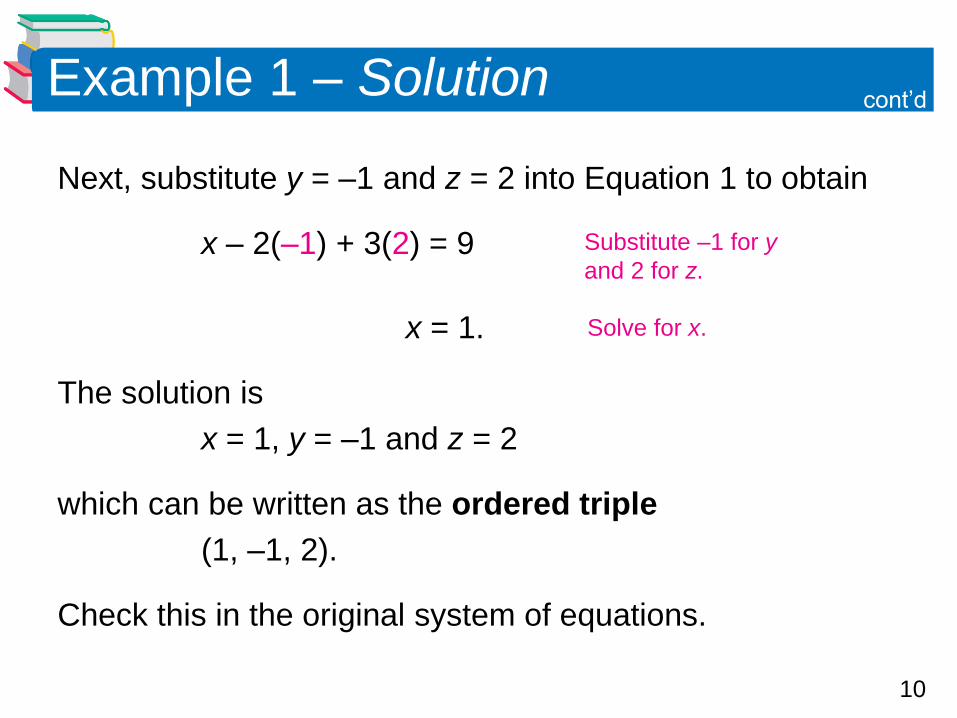
Next, substitute y = –1 and z = 2 into Equation 1 to obtain

x – 2(–1) + 3(2) = 9

x = 1.

The solution is

x = 1, y = –1 and z = 2

which can be written as the ordered triple

(1, –1, 2).

Check this in the original system of equations.

cont’d

Substitute –1 for y

and 2 for z.

Solve for x.

11

Gaussian Elimination

12

Gaussian Elimination

Two systems of equations are equivalent when they have

the same solution set.

To solve a system that is not in row-echelon form, first

convert it to an equivalent system that is in row-echelon

form by using one or more of the elementary row

operations shown below.

This process is called Gaussian elimination, after the

German mathematician Carl Friedrich Gauss (1777–1855).

13

Gaussian Elimination

14

Example 2 – Using Gaussian Elimination to Solve a System

Solve the system of linear equations.

x – 2y + 3z = 9

–x + 3y + z = –2

2x – 5y + 5z = 17

Solution:

Because the leading coefficient of the first equation is 1,

you can begin by saving the x at the upper left and

eliminating the other x-terms from the first column.

Equation 1

Equation 2

Equation 3

15

Example 2 – Solution

x – 2y + 3z = 9

y + 4z = 7

2x – 5y + 5z = 17

x – 2y + 3z = 9

y + 4z = 7

– y – z = –1

Now that all but the first x have been eliminated from the

first column, go to work on the second column. (You need

to eliminate y from the third equation.)

cont’d

16

Example 2 – Solution

x – 2y + 3z = 9

y + 4z = 7

3z = 6

Finally, you need a coefficient of 1 for z in the third

equation.

x – 2y + 3z = 9

y + 4z = 7

z = 2

cont’d

17

Gaussian Elimination

A system of linear equations is called consistent when it

has at least one solution. A consistent system with exactly

one solution is independent.

A consistent system with infinitely many solutions is

dependent. A system of linear equations is called

inconsistent when it has no solution.

18

Nonsquare Systems

19

Nonsquare Systems

So far, each system of linear equations you have looked at

has been square, which means that the number of

equations is equal to the number of variables.

In a nonsquare system of equations, the number of

equations differs from the number of variables.

A system of linear equations cannot have a unique solution

unless there are at least as many equations as there are

variables in the system.

20

Example 5 – A System with Fewer Equations than Variables

Solve the system of linear equations.

x – 2y + z = 2

2x – y – z = 1

Solution:

Begin by rewriting the system in row-echelon form.

x – 2y + z = 2

3y – 3z = –3

x – 2y + z = 2

y – z = –1

Equation 1

Equation 2

21

Example 5 – Solution

Solve for y in terms of z to obtain

y = z – 1.

By back-substituting into Equation 1, you can solve for x as

follows.

x – 2y + z = 2

x – 2(z – 1) + z = 2

x – 2z + 2 + z = 2

x = z

cont’d

Write Equation 1

Substitute z – 1 for y.

Distributive Property

Solve for x.

22

Example 5 – Solution

Finally, by letting z = a, where a is a real number, you have

the solution

x = a, y = a – 1, and z = a.

So, every ordered triple of the form

(a, a – 1, a)

is a solution of the system.

cont’d

a is a real number.

23

Graphical Interpretation of

Three-Variable Systems

24

Graphical Interpretation of Three-Variable Systems

Solutions of equations in three variables can be

represented graphically using a three-dimensional

coordinate system.

To construct such a system, begin with the xy-coordinate

plane in a horizontal position. Then draw the z-axis as a

vertical line through the origin.

Every ordered triple (x, y, z) corresponds to a point on the

three-dimensional coordinate system.

25

Graphical Interpretation of Three-Variable Systems

For instance, the points corresponding to (–2, 5, 4),

(2, –5, 3), and (3, 3, –2) are shown in Figure 7.7.

Figure 7.7

26

Graphical Interpretation of Three-Variable Systems

The graph of an equation in three variables consists of

all points (x, y, z) that are solutions of the equation. The

graph of a linear equation in three variables is a plane.

Sketching graphs on a three-dimensional coordinate

system is difficult because the sketch itself is only

two-dimensional.

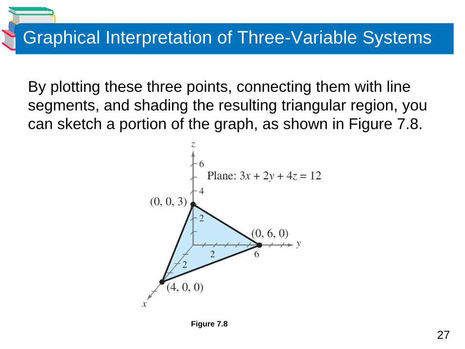
One technique for sketching a plane is to find the three

points at which the plane intersects the axes. For instance,

the plane

3x + 2y + 4z = 12

intersects the x-axis at the point (4, 0, 0), the y-axis at the

point (0, 6, 0), and the z-axis at the point (0, 0, 3).

27

Graphical Interpretation of Three-Variable Systems

By plotting these three points, connecting them with line

segments, and shading the resulting triangular region, you

can sketch a portion of the graph, as shown in Figure 7.8.

Figure 7.8

28

Graphical Interpretation of Three-Variable Systems

The graph of a system of three linear equations in three

variables consists of three planes. When these planes

intersect in a single point, the system has exactly one

solution (see Figure 7.9).

Figure 7.9

Solution: One point

29

Graphical Interpretation of Three-Variable Systems

When the three planes have no point in common, the

system has no solution (see Figures 7.10 and 7.11).

Figure 7.10

Solution: None

Figure 7.11

Solution: None

30

Graphical Interpretation of Three-Variable Systems

When the three planes intersect in a line or a plane, the

system has infinitely many solutions

(see Figures 7.12 and 7.13).

Figure 7.12

Solution: One line

Figure 7.13

Solution: One plane

31

Partial Fraction Decomposition

32

Partial Fraction Decomposition

A rational expression can often be written as the sum of

two or more simpler rational expressions. For example, the

rational expression

can be written as the sum of two fractions with linear

denominators. That is,

33

Partial Fraction Decomposition

Each fraction on the right side of the equation is a partial

fraction, and together they make up the partial fraction

decomposition of the left side.

34

Partial Fraction Decomposition

35

Example 6 – Distinct Linear Factors

Write the partial fraction decomposition of

Solution:

The expression is proper, so factor the denominator.

Because

x2 – x – 6 = (x – 3)(x + 2)

you should include one partial fraction with a constant

numerator for each linear factor of the denominator and

write

36

Example 6 – Solution

Multiplying each side of this equation by (x – 3)(x + 2), the

least common denominator (LCD), leads to the basic

equation

x + 7 = A(x + 2) + B(x – 3)

= Ax + 2A + Bx – 3B

= (A + B)x + 2A – 3B.

Because two polynomials are equal if and only if the

coefficients of like terms are equal, you can equate the

coefficients of like terms to opposite sides of the equation.

x + 7 = (A + B)x + ( 2A – 3B)

cont’d

Basic equation

Distributive Property

Write in polynomial form.

Equate coefficients

of like terms.

37

Example 6 – Solution

You can now write the following system of linear equations.

A + B = 1

2A – 3B = 7

You can solve the system of linear equations as follows.

From this equation, you can see that

A = 2.

cont’d

Equation 1

Equation 2

Multiply Equation 1 by 3.

Write Equation 2.

Add equations.

38

Example 6 – Solution

By back-substituting this value of A into Equation 1, you

can solve for B as follows.

A + B = 1

2 + B = 1

B = –1

So, the partial fraction decomposition is

Check this result by combining the two partial fractions on

the right side of the equation, or by using a graphing utility.

cont’d

Write Equation 1.

Substitute 2 for A.

Solve for B.

39

Applications

40

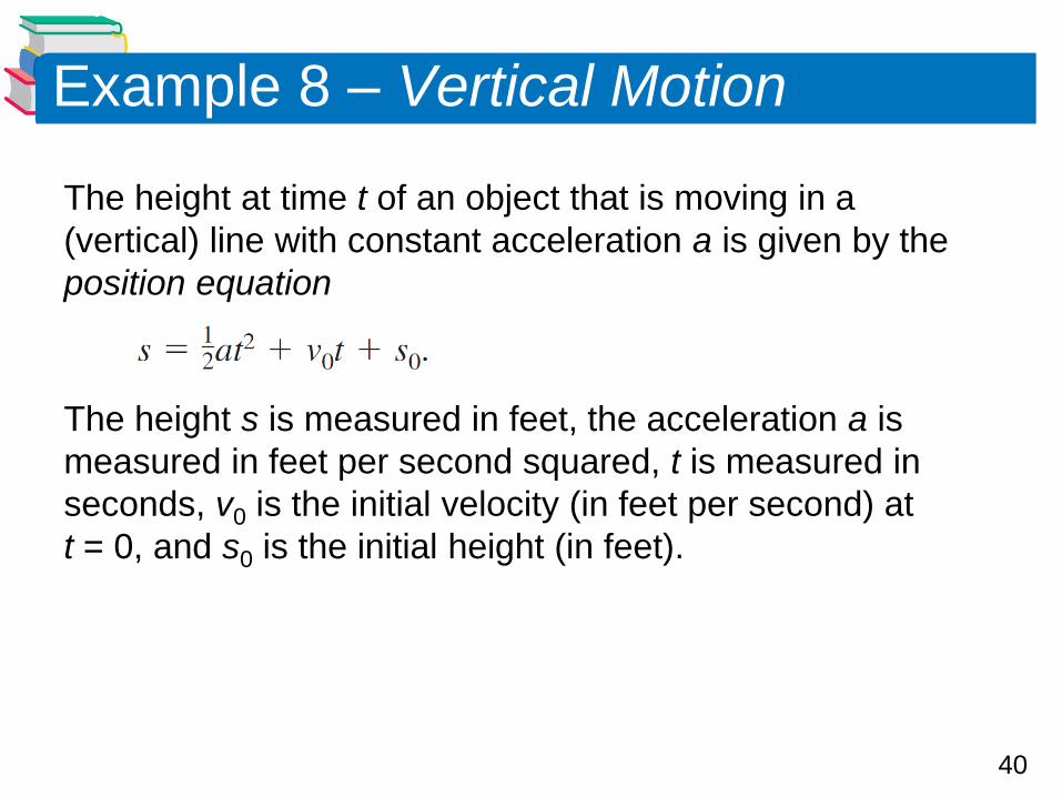
Example 8 – Vertical Motion

The height at time t of an object that is moving in a

(vertical) line with constant acceleration a is given by the

position equation

The height s is measured in feet, the acceleration a is

measured in feet per second squared, t is measured in

seconds, v0 is the initial velocity (in feet per second) at

t = 0, and s0 is the initial height (in feet).

41

Example 8 – Vertical Motion

Find the values of a, v0 and s0 when

s = 52 at t = 1, s = 52 at t = 2, and s = 20 at t = 3

and interpret the result.

(See Figure 7.14.)

Figure 7.14

cont’d

42

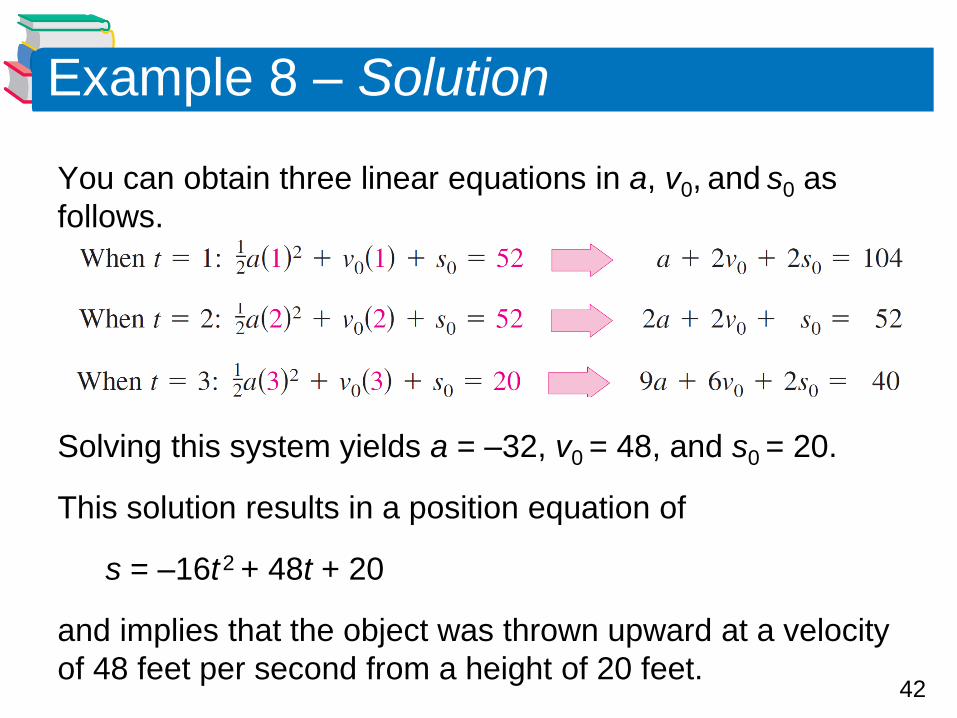
Example 8 – Solution

You can obtain three linear equations in a, v0, and s0 as

follows.

Solving this system yields a = –32, v0 = 48, and s0 = 20.

This solution results in a position equation of

s = –16t 2 + 48t + 20

and implies that the object was thrown upward at a velocity

of 48 feet per second from a height of 20 feet.

43

Homework:

Page 499

#’s 9, 21, 25, 49, 93