
7: Geometric Algorithms - University of Cambridge · Outline Introduction and Line Intersection...
316
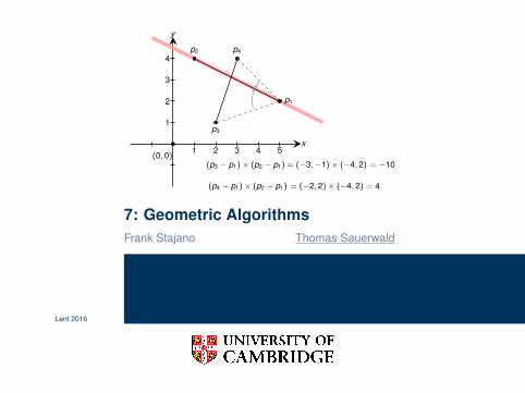
7: Geometric Algorithms Frank Stajano Thomas Sauerwald Lent 2016 x y 1 2 3 4 1 2 3 4 5 (0, 0) p3 p4 p2 p1 (p3 - p1) ⇥ (p2 - p1)=(-3, -1) ⇥ (-4, 2)= -10 (p4 - p1) ⇥ (p2 - p1)=(-2, 2) ⇥ (-4, 2)= 4
Transcript of 7: Geometric Algorithms - University of Cambridge · Outline Introduction and Line Intersection...
7: Geometric AlgorithmsFrank Stajano Thomas Sauerwald
Lent 2016
Solving Line Intersection (without Trigonometry and Division!)
x
y
1
2
3
4
1 2 3 4 5(0, 0)
p3
p4p2
p1
(p1 � p3)⇥ (p4 � p3) = (3, 1)⇥ (1, 3) = 8
(p2 � p3)⇥ (p4 � p3) = (�1, 3)⇥ (1, 3) = �6
Opposite signs ) p1p2 crosses(infinite) line through p3 and p4
Opposite signs ) p1p2 crosses(infinite) line through p3 and p4
(p3 � p1)⇥ (p2 � p1) = (�3,�1)⇥ (�4, 2) = �10
(p4 � p1)⇥ (p2 � p1) = (�2, 2)⇥ (�4, 2) = 4
Opposite signs ) p3p4 crosses(infinite) line through p1 and p2
Opposite signs ) p3p4 crosses(infinite) line through p1 and p2
p1p2 crosses p3p4
p3
p4
(p3 � p1)⇥ (p2 � p1) < 0
(p4 � p1)⇥ (p2 � p1) < 0
p1p2 does not cross p3p4
7: Geometric Algorithms T.S. 21
Outline
Introduction and Line Intersection
Convex Hull
Glimpse at (More) Advanced Algorithms
7: Geometric Algorithms T.S. 2
Introduction
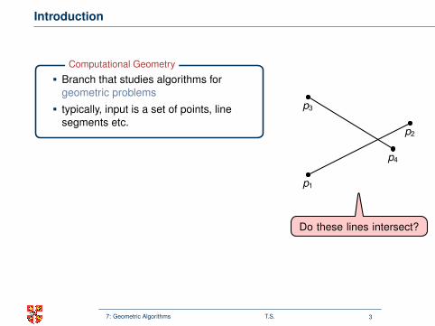
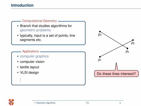
Branch that studies algorithms forgeometric problems
typically, input is a set of points, linesegments etc.
Computational Geometry
computer graphics
computer vision
textile layout
VLSI design...
Applications
p1
p2
p3
p4
Do these lines intersect?
7: Geometric Algorithms T.S. 3

Introduction
Branch that studies algorithms forgeometric problems
typically, input is a set of points, linesegments etc.
Computational Geometry
computer graphics
computer vision
textile layout
VLSI design...
Applications
p1
p2
p3
p4
Do these lines intersect?
7: Geometric Algorithms T.S. 3
Introduction
Branch that studies algorithms forgeometric problems
typically, input is a set of points, linesegments etc.
Computational Geometry
computer graphics
computer vision
textile layout
VLSI design...
Applications
p1
p2
p3
p4
Do these lines intersect?
7: Geometric Algorithms T.S. 3
Introduction
Branch that studies algorithms forgeometric problems
typically, input is a set of points, linesegments etc.
Computational Geometry
computer graphics
computer vision
textile layout
VLSI design...
Applications
p1
p2
p3
p4
Do these lines intersect?
7: Geometric Algorithms T.S. 3
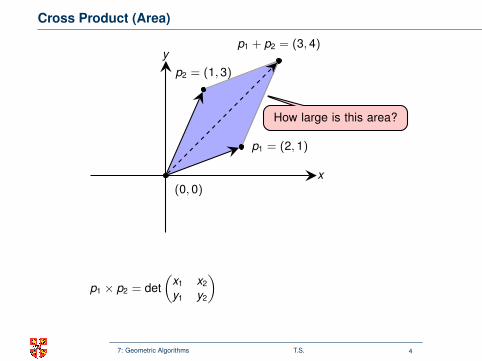
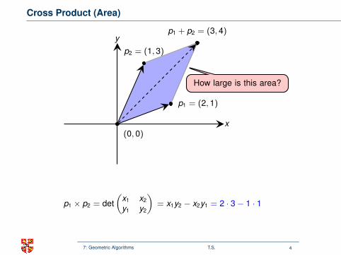
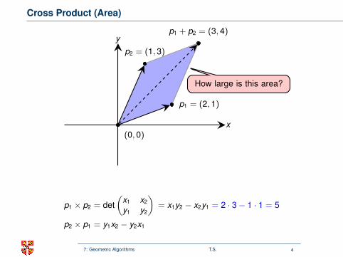
Cross Product (Area)
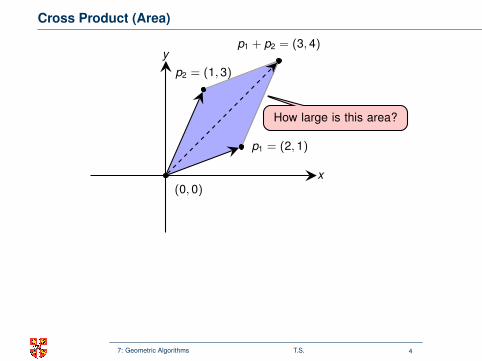
How large is this area?
x
y
(0, 0)
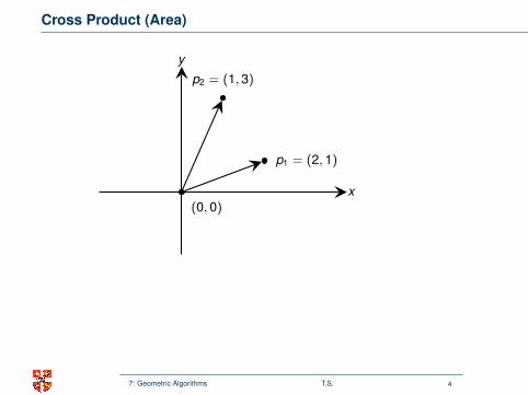
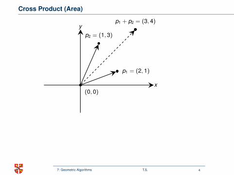
p1 = (2, 1)
p2 = (1, 3)
p1 + p2 = (3, 4)
Alternatively, one could take the dot-product (but not used here):p1 · p2 = ‖p1‖ · ‖p2‖ · cos(φ).
p1 × p2 = det(
x1 x2
y1 y2
)
= x1y2 − x2y1 = 2 · 3− 1 · 1
= 5
p2 × p1
= y1x2 − y2x1 = −(p1 × p2) = −5
7: Geometric Algorithms T.S. 4
Cross Product (Area)
How large is this area?
x
y
(0, 0)
p1 = (2, 1)
p2 = (1, 3)
p1 + p2 = (3, 4)
Alternatively, one could take the dot-product (but not used here):p1 · p2 = ‖p1‖ · ‖p2‖ · cos(φ).
p1 × p2 = det(
x1 x2
y1 y2
)
= x1y2 − x2y1 = 2 · 3− 1 · 1
= 5
p2 × p1
= y1x2 − y2x1 = −(p1 × p2) = −5
7: Geometric Algorithms T.S. 4

Cross Product (Area)
How large is this area?
x
y
(0, 0)
p1 = (2, 1)
p2 = (1, 3)
p1 + p2 = (3, 4)
Alternatively, one could take the dot-product (but not used here):p1 · p2 = ‖p1‖ · ‖p2‖ · cos(φ).
p1 × p2 = det(
x1 x2
y1 y2
)= x1y2 − x2y1
= 2 · 3− 1 · 1
= 5
p2 × p1
= y1x2 − y2x1 = −(p1 × p2) = −5
7: Geometric Algorithms T.S. 4
Cross Product (Area)
How large is this area?
x
y
(0, 0)
p1 = (2, 1)
p2 = (1, 3)
p1 + p2 = (3, 4)
Alternatively, one could take the dot-product (but not used here):p1 · p2 = ‖p1‖ · ‖p2‖ · cos(φ).
p1 × p2 = det(
x1 x2
y1 y2
)= x1y2 − x2y1 = 2 · 3− 1 · 1
= 5
p2 × p1
= y1x2 − y2x1 = −(p1 × p2) = −5
7: Geometric Algorithms T.S. 4

Cross Product (Area)
How large is this area?
x
y
(0, 0)
p1 = (2, 1)
p2 = (1, 3)
p1 + p2 = (3, 4)
Alternatively, one could take the dot-product (but not used here):p1 · p2 = ‖p1‖ · ‖p2‖ · cos(φ).
p1 × p2 = det(
x1 x2
y1 y2
)= x1y2 − x2y1 = 2 · 3− 1 · 1 = 5
p2 × p1
= y1x2 − y2x1 = −(p1 × p2) = −5
7: Geometric Algorithms T.S. 4
Cross Product (Area)
How large is this area?
x
y
(0, 0)
p1 = (2, 1)
p2 = (1, 3)
p1 + p2 = (3, 4)
Alternatively, one could take the dot-product (but not used here):p1 · p2 = ‖p1‖ · ‖p2‖ · cos(φ).
p1 × p2 = det(
x1 x2
y1 y2
)= x1y2 − x2y1 = 2 · 3− 1 · 1 = 5
p2 × p1 = y1x2 − y2x1
= −(p1 × p2) = −5
7: Geometric Algorithms T.S. 4

Cross Product (Area)
How large is this area?
x
y
(0, 0)
p1 = (2, 1)
p2 = (1, 3)
p1 + p2 = (3, 4)
Alternatively, one could take the dot-product (but not used here):p1 · p2 = ‖p1‖ · ‖p2‖ · cos(φ).
p1 × p2 = det(
x1 x2
y1 y2
)= x1y2 − x2y1 = 2 · 3− 1 · 1 = 5
p2 × p1 = y1x2 − y2x1 = −(p1 × p2)
= −5
7: Geometric Algorithms T.S. 4

Cross Product (Area)
How large is this area?
x
y
(0, 0)
p1 = (2, 1)
p2 = (1, 3)
p1 + p2 = (3, 4)
Alternatively, one could take the dot-product (but not used here):p1 · p2 = ‖p1‖ · ‖p2‖ · cos(φ).
p1 × p2 = det(
x1 x2
y1 y2
)= x1y2 − x2y1 = 2 · 3− 1 · 1 = 5
p2 × p1 = y1x2 − y2x1 = −(p1 × p2) = −5
7: Geometric Algorithms T.S. 4
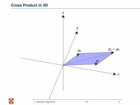
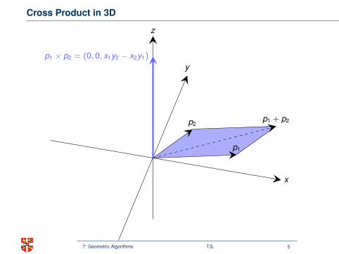
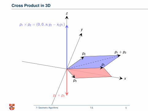
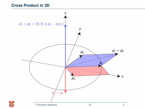
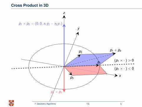
Cross Product in 3D
y
x
z
p1
p2
p3
p1 + p2
p1 × p2 = (0, 0, x1y2 − x2y1)
p1 × p3
(p1 × · ) > 0
(p1 × · ) < 0
7: Geometric Algorithms T.S. 5
Cross Product in 3D
y
x
z
p1
p2
p3
p1 + p2
p1 × p2 = (0, 0, x1y2 − x2y1)
p1 × p3
(p1 × · ) > 0
(p1 × · ) < 0
7: Geometric Algorithms T.S. 5

Cross Product in 3D
y
x
z
p1
p2
p3
p1 + p2
p1 × p2 = (0, 0, x1y2 − x2y1)
p1 × p3
(p1 × · ) > 0
(p1 × · ) < 0
7: Geometric Algorithms T.S. 5
Cross Product in 3D
y
x
z
p1
p2
p3
p1 + p2
p1 × p2 = (0, 0, x1y2 − x2y1)
p1 × p3
(p1 × · ) > 0
(p1 × · ) < 0
7: Geometric Algorithms T.S. 5
Cross Product in 3D
y
x
z
p1
p2
p3
p1 + p2
p1 × p2 = (0, 0, x1y2 − x2y1)
p1 × p3
(p1 × · ) > 0
(p1 × · ) < 0
7: Geometric Algorithms T.S. 5
Cross Product in 3D
y
x
z
p1
p2
p3
p1 + p2
p1 × p2 = (0, 0, x1y2 − x2y1)
p1 × p3
(p1 × · ) > 0
(p1 × · ) < 0
7: Geometric Algorithms T.S. 5
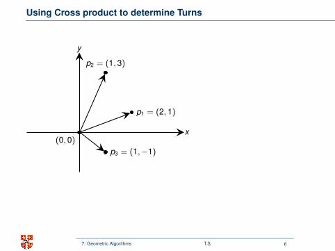
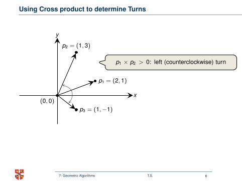
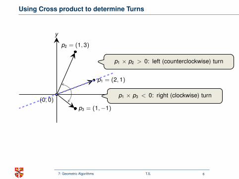
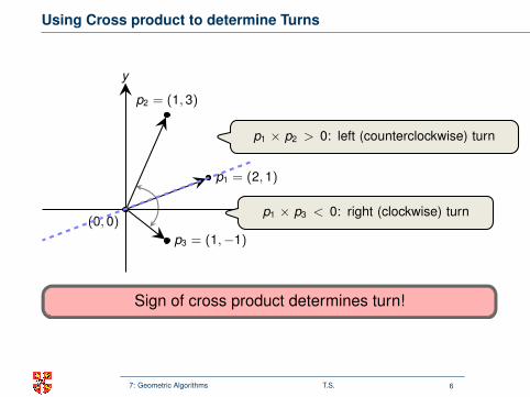
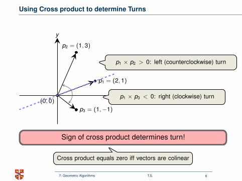
Using Cross product to determine Turns
x
y
(0, 0)
p1 = (2, 1)
p2 = (1, 3)
p3 = (1,−1)
p1 × p2 > 0: left (counterclockwise) turn
p1 × p3 < 0: right (clockwise) turn
Sign of cross product determines turn!
Cross product equals zero iff vectors are colinear
7: Geometric Algorithms T.S. 6

Using Cross product to determine Turns
x
y
(0, 0)
p1 = (2, 1)
p2 = (1, 3)
p3 = (1,−1)
p1 × p2 > 0: left (counterclockwise) turn
p1 × p3 < 0: right (clockwise) turn
Sign of cross product determines turn!
Cross product equals zero iff vectors are colinear
7: Geometric Algorithms T.S. 6

Using Cross product to determine Turns
x
y
(0, 0)
p1 = (2, 1)
p2 = (1, 3)
p3 = (1,−1)
p1 × p2 > 0: left (counterclockwise) turn
p1 × p3 < 0: right (clockwise) turn
Sign of cross product determines turn!
Cross product equals zero iff vectors are colinear
7: Geometric Algorithms T.S. 6
Using Cross product to determine Turns
x
y
(0, 0)
p1 = (2, 1)
p2 = (1, 3)
p3 = (1,−1)
p1 × p2 > 0: left (counterclockwise) turn
p1 × p3 < 0: right (clockwise) turn
Sign of cross product determines turn!
Cross product equals zero iff vectors are colinear
7: Geometric Algorithms T.S. 6

Using Cross product to determine Turns
x
y
(0, 0)
p1 = (2, 1)
p2 = (1, 3)
p3 = (1,−1)
p1 × p2 > 0: left (counterclockwise) turn
p1 × p3 < 0: right (clockwise) turn
Sign of cross product determines turn!
Cross product equals zero iff vectors are colinear
7: Geometric Algorithms T.S. 6
Using Cross product to determine Turns
x
y
(0, 0)
p1 = (2, 1)
p2 = (1, 3)
p3 = (1,−1)
p1 × p2 > 0: left (counterclockwise) turn
p1 × p3 < 0: right (clockwise) turn
Sign of cross product determines turn!
Cross product equals zero iff vectors are colinear
7: Geometric Algorithms T.S. 6
Using Cross product to determine Turns
x
y
(0, 0)
p1 = (2, 1)
p2 = (1, 3)
p3 = (1,−1)
p1 × p2 > 0: left (counterclockwise) turn
p1 × p3 < 0: right (clockwise) turn
Sign of cross product determines turn!
Cross product equals zero iff vectors are colinear
7: Geometric Algorithms T.S. 6
Using Cross product to determine Turns
x
y
(0, 0)
p1 = (2, 1)
p2 = (1, 3)
p3 = (1,−1)
p1 × p2 > 0: left (counterclockwise) turn
p1 × p3 < 0: right (clockwise) turn
Sign of cross product determines turn!
Cross product equals zero iff vectors are colinear
7: Geometric Algorithms T.S. 6
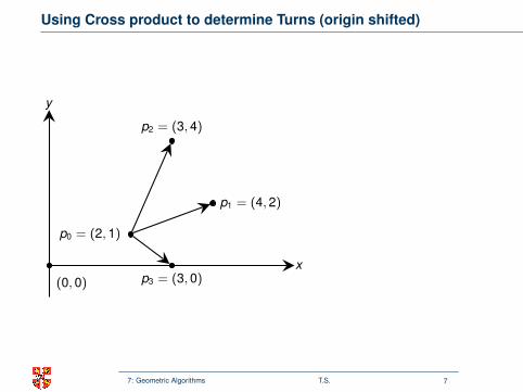
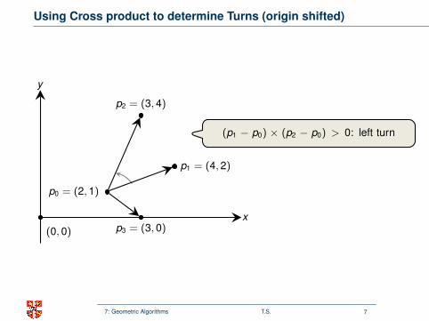
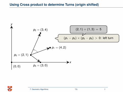
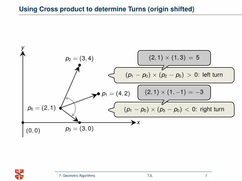
Using Cross product to determine Turns (origin shifted)
x
y
p0 = (2, 1)
(0, 0)
p1 = (4, 2)
p2 = (3, 4)
p3 = (3, 0)
(p1 − p0) × (p2 − p0) > 0: left turn
(2, 1) × (1, 3) = 5
(p1 − p0) × (p3 − p0) < 0: right turn
(2, 1) × (1,−1) = −3
7: Geometric Algorithms T.S. 7

Using Cross product to determine Turns (origin shifted)
x
y
p0 = (2, 1)
(0, 0)
p1 = (4, 2)
p2 = (3, 4)
p3 = (3, 0)
(p1 − p0) × (p2 − p0) > 0: left turn
(2, 1) × (1, 3) = 5
(p1 − p0) × (p3 − p0) < 0: right turn
(2, 1) × (1,−1) = −3
7: Geometric Algorithms T.S. 7
Using Cross product to determine Turns (origin shifted)
x
y
p0 = (2, 1)
(0, 0)
p1 = (4, 2)
p2 = (3, 4)
p3 = (3, 0)
(p1 − p0) × (p2 − p0) > 0: left turn
(2, 1) × (1, 3) = 5
(p1 − p0) × (p3 − p0) < 0: right turn
(2, 1) × (1,−1) = −3
7: Geometric Algorithms T.S. 7
Using Cross product to determine Turns (origin shifted)
x
y
p0 = (2, 1)
(0, 0)
p1 = (4, 2)
p2 = (3, 4)
p3 = (3, 0)
(p1 − p0) × (p2 − p0) > 0: left turn
(2, 1) × (1, 3) = 5
(p1 − p0) × (p3 − p0) < 0: right turn
(2, 1) × (1,−1) = −3
7: Geometric Algorithms T.S. 7

Using Cross product to determine Turns (origin shifted)
x
y
p0 = (2, 1)
(0, 0)
p1 = (4, 2)
p2 = (3, 4)
p3 = (3, 0)
(p1 − p0) × (p2 − p0) > 0: left turn
(2, 1) × (1, 3) = 5
(p1 − p0) × (p3 − p0) < 0: right turn
(2, 1) × (1,−1) = −3
7: Geometric Algorithms T.S. 7

Using Cross product to determine Turns (origin shifted)
x
y
p0 = (2, 1)
(0, 0)
p1 = (4, 2)
p2 = (3, 4)
p3 = (3, 0)
(p1 − p0) × (p2 − p0) > 0: left turn
(2, 1) × (1, 3) = 5
(p1 − p0) × (p3 − p0) < 0: right turn
(2, 1) × (1,−1) = −3
7: Geometric Algorithms T.S. 7
Using Cross product to determine Turns (origin shifted)
x
y
p0 = (2, 1)
(0, 0)
p1 = (4, 2)
p2 = (3, 4)
p3 = (3, 0)
(p1 − p0) × (p2 − p0) > 0: left turn
(2, 1) × (1, 3) = 5
(p1 − p0) × (p3 − p0) < 0: right turn
(2, 1) × (1,−1) = −3
7: Geometric Algorithms T.S. 7

Using Cross product to determine Turns (origin shifted)
x
y
p0 = (2, 1)
(0, 0)
p1 = (4, 2)
p2 = (3, 4)
p3 = (3, 0)
(p1 − p0) × (p2 − p0) > 0: left turn
(2, 1) × (1, 3) = 5
(p1 − p0) × (p3 − p0) < 0: right turn
(2, 1) × (1,−1) = −3
7: Geometric Algorithms T.S. 7
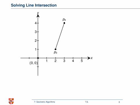
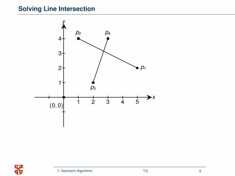
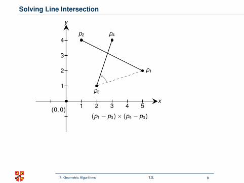
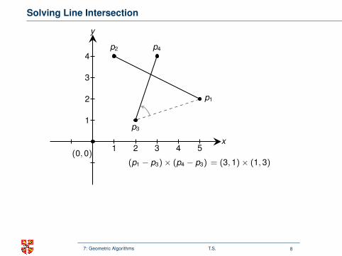
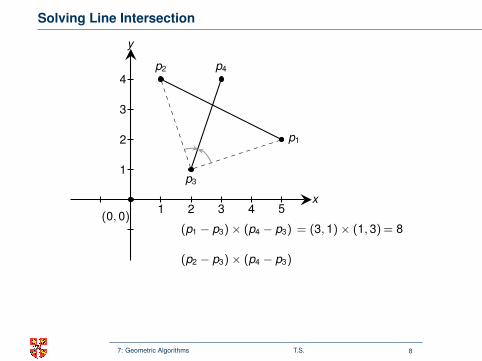
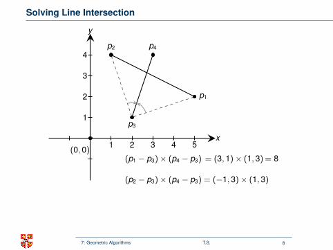
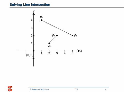
Solving Line Intersection
x
y
1
2
3
4
1 2 3 4 5(0, 0)
p3
p4p2
p1
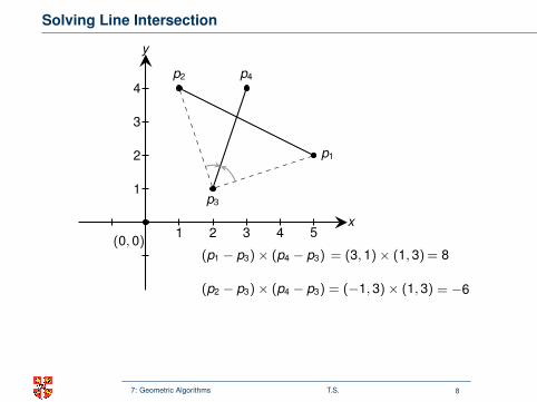
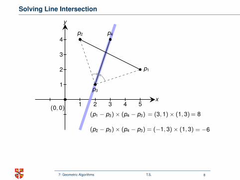
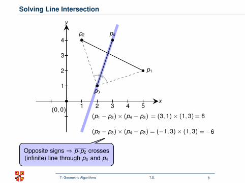
(p1 − p3)× (p4 − p3) = (3, 1)× (1, 3) = 8
(p2 − p3)× (p4 − p3) = (−1, 3)× (1, 3) = −6
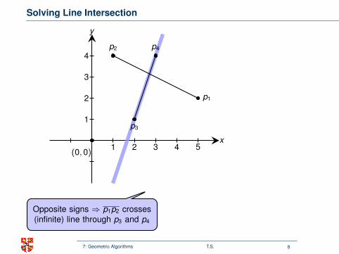
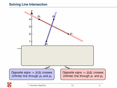
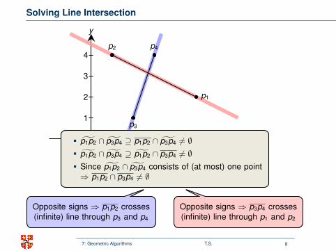
Opposite signs ⇒ p1p2 crosses(infinite) line through p3 and p4
Opposite signs ⇒ p1p2 crosses(infinite) line through p3 and p4
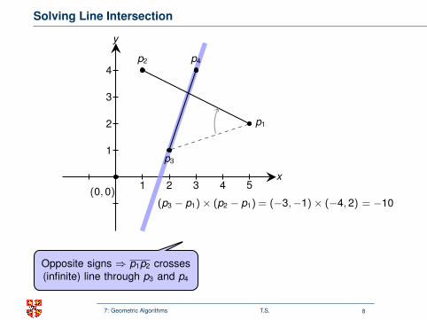
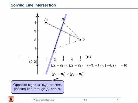
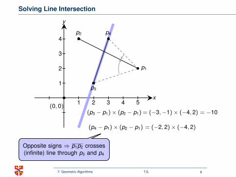
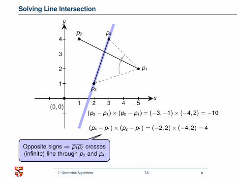
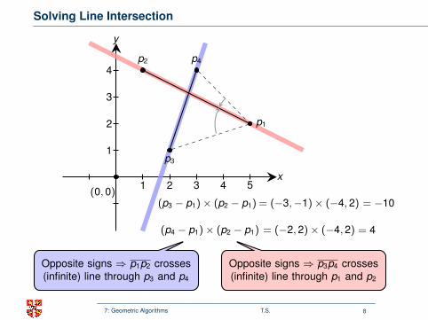
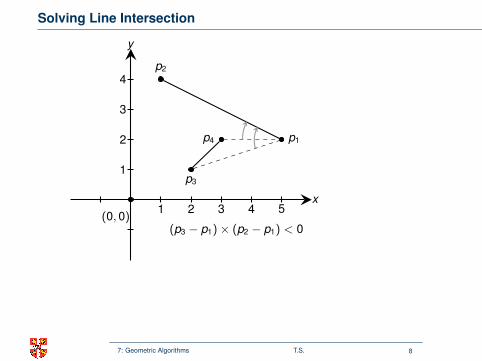
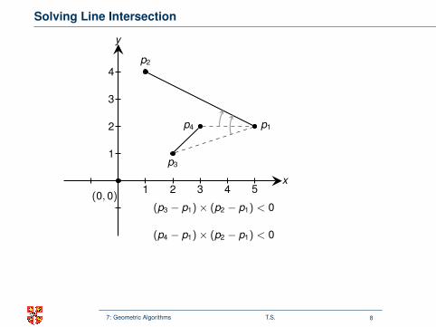
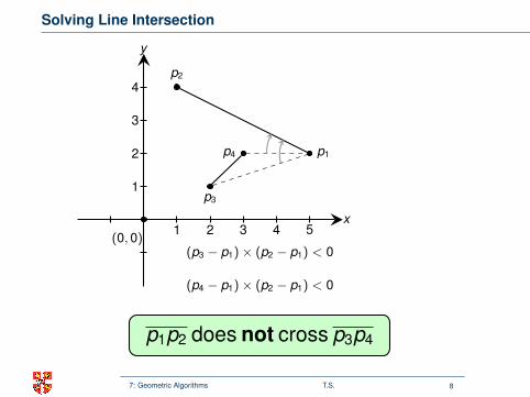
(p3 − p1)× (p2 − p1) = (−3,−1)× (−4, 2) = −10
(p4 − p1)× (p2 − p1) = (−2, 2)× (−4, 2) = 4
Opposite signs ⇒ p3p4 crosses(infinite) line through p1 and p2
Opposite signs ⇒ p3p4 crosses(infinite) line through p1 and p2
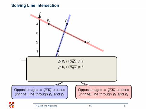
p̃1p2 ∩ p̃3p4 ⊇
p1p2 ∩ p̃3p4 6= ∅
p̃1p2 ∩ p̃3p4 ⊇
p̃1p2 ∩ p3p4 6= ∅Since p̃1p2 ∩ p̃3p4 consists of (at most) one point⇒ p1p2 ∩ p3p4 6= ∅
p1p2 crosses p3p4
p3
p4
(p3 − p1)× (p2 − p1) < 0
(p4 − p1)× (p2 − p1) < 0
p1p2 does not cross p3p4
7: Geometric Algorithms T.S. 8
Solving Line Intersection
x
y
1
2
3
4
1 2 3 4 5(0, 0)
p3
p4
p2
p1
(p1 − p3)× (p4 − p3) = (3, 1)× (1, 3) = 8
(p2 − p3)× (p4 − p3) = (−1, 3)× (1, 3) = −6
Opposite signs ⇒ p1p2 crosses(infinite) line through p3 and p4
Opposite signs ⇒ p1p2 crosses(infinite) line through p3 and p4
(p3 − p1)× (p2 − p1) = (−3,−1)× (−4, 2) = −10
(p4 − p1)× (p2 − p1) = (−2, 2)× (−4, 2) = 4
Opposite signs ⇒ p3p4 crosses(infinite) line through p1 and p2
Opposite signs ⇒ p3p4 crosses(infinite) line through p1 and p2
p̃1p2 ∩ p̃3p4 ⊇
p1p2 ∩ p̃3p4 6= ∅
p̃1p2 ∩ p̃3p4 ⊇
p̃1p2 ∩ p3p4 6= ∅Since p̃1p2 ∩ p̃3p4 consists of (at most) one point⇒ p1p2 ∩ p3p4 6= ∅
p1p2 crosses p3p4
p3
p4
(p3 − p1)× (p2 − p1) < 0
(p4 − p1)× (p2 − p1) < 0
p1p2 does not cross p3p4
7: Geometric Algorithms T.S. 8
Solving Line Intersection
x
y
1
2
3
4
1 2 3 4 5(0, 0)
p3
p4p2
p1
(p1 − p3)× (p4 − p3)
= (3, 1)× (1, 3) = 8
(p2 − p3)× (p4 − p3) = (−1, 3)× (1, 3) = −6
Opposite signs ⇒ p1p2 crosses(infinite) line through p3 and p4
Opposite signs ⇒ p1p2 crosses(infinite) line through p3 and p4
(p3 − p1)× (p2 − p1) = (−3,−1)× (−4, 2) = −10
(p4 − p1)× (p2 − p1) = (−2, 2)× (−4, 2) = 4
Opposite signs ⇒ p3p4 crosses(infinite) line through p1 and p2
Opposite signs ⇒ p3p4 crosses(infinite) line through p1 and p2
p̃1p2 ∩ p̃3p4 ⊇
p1p2 ∩ p̃3p4 6= ∅
p̃1p2 ∩ p̃3p4 ⊇
p̃1p2 ∩ p3p4 6= ∅Since p̃1p2 ∩ p̃3p4 consists of (at most) one point⇒ p1p2 ∩ p3p4 6= ∅
p1p2 crosses p3p4
p3
p4
(p3 − p1)× (p2 − p1) < 0
(p4 − p1)× (p2 − p1) < 0
p1p2 does not cross p3p4
7: Geometric Algorithms T.S. 8
Solving Line Intersection
x
y
1
2
3
4
1 2 3 4 5(0, 0)
p3
p4p2
p1
(p1 − p3)× (p4 − p3) = (3, 1)× (1, 3)
= 8
(p2 − p3)× (p4 − p3) = (−1, 3)× (1, 3) = −6
Opposite signs ⇒ p1p2 crosses(infinite) line through p3 and p4
Opposite signs ⇒ p1p2 crosses(infinite) line through p3 and p4
(p3 − p1)× (p2 − p1) = (−3,−1)× (−4, 2) = −10
(p4 − p1)× (p2 − p1) = (−2, 2)× (−4, 2) = 4
Opposite signs ⇒ p3p4 crosses(infinite) line through p1 and p2
Opposite signs ⇒ p3p4 crosses(infinite) line through p1 and p2
p̃1p2 ∩ p̃3p4 ⊇
p1p2 ∩ p̃3p4 6= ∅
p̃1p2 ∩ p̃3p4 ⊇
p̃1p2 ∩ p3p4 6= ∅Since p̃1p2 ∩ p̃3p4 consists of (at most) one point⇒ p1p2 ∩ p3p4 6= ∅
p1p2 crosses p3p4
p3
p4
(p3 − p1)× (p2 − p1) < 0
(p4 − p1)× (p2 − p1) < 0
p1p2 does not cross p3p4
7: Geometric Algorithms T.S. 8

Solving Line Intersection
x
y
1
2
3
4
1 2 3 4 5(0, 0)
p3
p4p2
p1
(p1 − p3)× (p4 − p3) = (3, 1)× (1, 3) = 8
(p2 − p3)× (p4 − p3) = (−1, 3)× (1, 3) = −6
Opposite signs ⇒ p1p2 crosses(infinite) line through p3 and p4
Opposite signs ⇒ p1p2 crosses(infinite) line through p3 and p4
(p3 − p1)× (p2 − p1) = (−3,−1)× (−4, 2) = −10
(p4 − p1)× (p2 − p1) = (−2, 2)× (−4, 2) = 4
Opposite signs ⇒ p3p4 crosses(infinite) line through p1 and p2
Opposite signs ⇒ p3p4 crosses(infinite) line through p1 and p2
p̃1p2 ∩ p̃3p4 ⊇
p1p2 ∩ p̃3p4 6= ∅
p̃1p2 ∩ p̃3p4 ⊇
p̃1p2 ∩ p3p4 6= ∅Since p̃1p2 ∩ p̃3p4 consists of (at most) one point⇒ p1p2 ∩ p3p4 6= ∅
p1p2 crosses p3p4
p3
p4
(p3 − p1)× (p2 − p1) < 0
(p4 − p1)× (p2 − p1) < 0
p1p2 does not cross p3p4
7: Geometric Algorithms T.S. 8
Solving Line Intersection
x
y
1
2
3
4
1 2 3 4 5(0, 0)
p3
p4p2
p1
(p1 − p3)× (p4 − p3) = (3, 1)× (1, 3) = 8
(p2 − p3)× (p4 − p3)
= (−1, 3)× (1, 3) = −6
Opposite signs ⇒ p1p2 crosses(infinite) line through p3 and p4
Opposite signs ⇒ p1p2 crosses(infinite) line through p3 and p4
(p3 − p1)× (p2 − p1) = (−3,−1)× (−4, 2) = −10
(p4 − p1)× (p2 − p1) = (−2, 2)× (−4, 2) = 4
Opposite signs ⇒ p3p4 crosses(infinite) line through p1 and p2
Opposite signs ⇒ p3p4 crosses(infinite) line through p1 and p2
p̃1p2 ∩ p̃3p4 ⊇
p1p2 ∩ p̃3p4 6= ∅
p̃1p2 ∩ p̃3p4 ⊇
p̃1p2 ∩ p3p4 6= ∅Since p̃1p2 ∩ p̃3p4 consists of (at most) one point⇒ p1p2 ∩ p3p4 6= ∅
p1p2 crosses p3p4
p3
p4
(p3 − p1)× (p2 − p1) < 0
(p4 − p1)× (p2 − p1) < 0
p1p2 does not cross p3p4
7: Geometric Algorithms T.S. 8
Solving Line Intersection
x
y
1
2
3
4
1 2 3 4 5(0, 0)
p3
p4p2
p1
(p1 − p3)× (p4 − p3) = (3, 1)× (1, 3) = 8
(p2 − p3)× (p4 − p3) = (−1, 3)× (1, 3)
= −6
Opposite signs ⇒ p1p2 crosses(infinite) line through p3 and p4
Opposite signs ⇒ p1p2 crosses(infinite) line through p3 and p4
(p3 − p1)× (p2 − p1) = (−3,−1)× (−4, 2) = −10
(p4 − p1)× (p2 − p1) = (−2, 2)× (−4, 2) = 4
Opposite signs ⇒ p3p4 crosses(infinite) line through p1 and p2
Opposite signs ⇒ p3p4 crosses(infinite) line through p1 and p2
p̃1p2 ∩ p̃3p4 ⊇
p1p2 ∩ p̃3p4 6= ∅
p̃1p2 ∩ p̃3p4 ⊇
p̃1p2 ∩ p3p4 6= ∅Since p̃1p2 ∩ p̃3p4 consists of (at most) one point⇒ p1p2 ∩ p3p4 6= ∅
p1p2 crosses p3p4
p3
p4
(p3 − p1)× (p2 − p1) < 0
(p4 − p1)× (p2 − p1) < 0
p1p2 does not cross p3p4
7: Geometric Algorithms T.S. 8
Solving Line Intersection
x
y
1
2
3
4
1 2 3 4 5(0, 0)
p3
p4p2
p1
(p1 − p3)× (p4 − p3) = (3, 1)× (1, 3) = 8
(p2 − p3)× (p4 − p3) = (−1, 3)× (1, 3) = −6
Opposite signs ⇒ p1p2 crosses(infinite) line through p3 and p4
Opposite signs ⇒ p1p2 crosses(infinite) line through p3 and p4
(p3 − p1)× (p2 − p1) = (−3,−1)× (−4, 2) = −10
(p4 − p1)× (p2 − p1) = (−2, 2)× (−4, 2) = 4
Opposite signs ⇒ p3p4 crosses(infinite) line through p1 and p2
Opposite signs ⇒ p3p4 crosses(infinite) line through p1 and p2
p̃1p2 ∩ p̃3p4 ⊇
p1p2 ∩ p̃3p4 6= ∅
p̃1p2 ∩ p̃3p4 ⊇
p̃1p2 ∩ p3p4 6= ∅Since p̃1p2 ∩ p̃3p4 consists of (at most) one point⇒ p1p2 ∩ p3p4 6= ∅
p1p2 crosses p3p4
p3
p4
(p3 − p1)× (p2 − p1) < 0
(p4 − p1)× (p2 − p1) < 0
p1p2 does not cross p3p4
7: Geometric Algorithms T.S. 8
Solving Line Intersection
x
y
1
2
3
4
1 2 3 4 5(0, 0)
p3
p4p2
p1
(p1 − p3)× (p4 − p3) = (3, 1)× (1, 3) = 8
(p2 − p3)× (p4 − p3) = (−1, 3)× (1, 3) = −6
Opposite signs ⇒ p1p2 crosses(infinite) line through p3 and p4
Opposite signs ⇒ p1p2 crosses(infinite) line through p3 and p4
(p3 − p1)× (p2 − p1) = (−3,−1)× (−4, 2) = −10
(p4 − p1)× (p2 − p1) = (−2, 2)× (−4, 2) = 4
Opposite signs ⇒ p3p4 crosses(infinite) line through p1 and p2
Opposite signs ⇒ p3p4 crosses(infinite) line through p1 and p2
p̃1p2 ∩ p̃3p4 ⊇
p1p2 ∩ p̃3p4 6= ∅
p̃1p2 ∩ p̃3p4 ⊇
p̃1p2 ∩ p3p4 6= ∅Since p̃1p2 ∩ p̃3p4 consists of (at most) one point⇒ p1p2 ∩ p3p4 6= ∅
p1p2 crosses p3p4
p3
p4
(p3 − p1)× (p2 − p1) < 0
(p4 − p1)× (p2 − p1) < 0
p1p2 does not cross p3p4
7: Geometric Algorithms T.S. 8

Solving Line Intersection
x
y
1
2
3
4
1 2 3 4 5(0, 0)
p3
p4p2
p1
(p1 − p3)× (p4 − p3) = (3, 1)× (1, 3) = 8
(p2 − p3)× (p4 − p3) = (−1, 3)× (1, 3) = −6
Opposite signs ⇒ p1p2 crosses(infinite) line through p3 and p4
Opposite signs ⇒ p1p2 crosses(infinite) line through p3 and p4
(p3 − p1)× (p2 − p1)
= (−3,−1)× (−4, 2) = −10
(p4 − p1)× (p2 − p1) = (−2, 2)× (−4, 2) = 4
Opposite signs ⇒ p3p4 crosses(infinite) line through p1 and p2
Opposite signs ⇒ p3p4 crosses(infinite) line through p1 and p2
p̃1p2 ∩ p̃3p4 ⊇
p1p2 ∩ p̃3p4 6= ∅
p̃1p2 ∩ p̃3p4 ⊇
p̃1p2 ∩ p3p4 6= ∅Since p̃1p2 ∩ p̃3p4 consists of (at most) one point⇒ p1p2 ∩ p3p4 6= ∅
p1p2 crosses p3p4
p3
p4
(p3 − p1)× (p2 − p1) < 0
(p4 − p1)× (p2 − p1) < 0
p1p2 does not cross p3p4
7: Geometric Algorithms T.S. 8

Solving Line Intersection
x
y
1
2
3
4
1 2 3 4 5(0, 0)
p3
p4p2
p1
(p1 − p3)× (p4 − p3) = (3, 1)× (1, 3) = 8
(p2 − p3)× (p4 − p3) = (−1, 3)× (1, 3) = −6
Opposite signs ⇒ p1p2 crosses(infinite) line through p3 and p4
Opposite signs ⇒ p1p2 crosses(infinite) line through p3 and p4
(p3 − p1)× (p2 − p1) = (−3,−1)× (−4, 2)
= −10
(p4 − p1)× (p2 − p1) = (−2, 2)× (−4, 2) = 4
Opposite signs ⇒ p3p4 crosses(infinite) line through p1 and p2
Opposite signs ⇒ p3p4 crosses(infinite) line through p1 and p2
p̃1p2 ∩ p̃3p4 ⊇
p1p2 ∩ p̃3p4 6= ∅
p̃1p2 ∩ p̃3p4 ⊇
p̃1p2 ∩ p3p4 6= ∅Since p̃1p2 ∩ p̃3p4 consists of (at most) one point⇒ p1p2 ∩ p3p4 6= ∅
p1p2 crosses p3p4
p3
p4
(p3 − p1)× (p2 − p1) < 0
(p4 − p1)× (p2 − p1) < 0
p1p2 does not cross p3p4
7: Geometric Algorithms T.S. 8
Solving Line Intersection
x
y
1
2
3
4
1 2 3 4 5(0, 0)
p3
p4p2
p1
(p1 − p3)× (p4 − p3) = (3, 1)× (1, 3) = 8
(p2 − p3)× (p4 − p3) = (−1, 3)× (1, 3) = −6
Opposite signs ⇒ p1p2 crosses(infinite) line through p3 and p4
Opposite signs ⇒ p1p2 crosses(infinite) line through p3 and p4
(p3 − p1)× (p2 − p1) = (−3,−1)× (−4, 2) = −10
(p4 − p1)× (p2 − p1) = (−2, 2)× (−4, 2) = 4
Opposite signs ⇒ p3p4 crosses(infinite) line through p1 and p2
Opposite signs ⇒ p3p4 crosses(infinite) line through p1 and p2
p̃1p2 ∩ p̃3p4 ⊇
p1p2 ∩ p̃3p4 6= ∅
p̃1p2 ∩ p̃3p4 ⊇
p̃1p2 ∩ p3p4 6= ∅Since p̃1p2 ∩ p̃3p4 consists of (at most) one point⇒ p1p2 ∩ p3p4 6= ∅
p1p2 crosses p3p4
p3
p4
(p3 − p1)× (p2 − p1) < 0
(p4 − p1)× (p2 − p1) < 0
p1p2 does not cross p3p4
7: Geometric Algorithms T.S. 8
Solving Line Intersection
x
y
1
2
3
4
1 2 3 4 5(0, 0)
p3
p4p2
p1
(p1 − p3)× (p4 − p3) = (3, 1)× (1, 3) = 8
(p2 − p3)× (p4 − p3) = (−1, 3)× (1, 3) = −6
Opposite signs ⇒ p1p2 crosses(infinite) line through p3 and p4
Opposite signs ⇒ p1p2 crosses(infinite) line through p3 and p4
(p3 − p1)× (p2 − p1) = (−3,−1)× (−4, 2) = −10
(p4 − p1)× (p2 − p1)
= (−2, 2)× (−4, 2) = 4
Opposite signs ⇒ p3p4 crosses(infinite) line through p1 and p2
Opposite signs ⇒ p3p4 crosses(infinite) line through p1 and p2
p̃1p2 ∩ p̃3p4 ⊇
p1p2 ∩ p̃3p4 6= ∅
p̃1p2 ∩ p̃3p4 ⊇
p̃1p2 ∩ p3p4 6= ∅Since p̃1p2 ∩ p̃3p4 consists of (at most) one point⇒ p1p2 ∩ p3p4 6= ∅
p1p2 crosses p3p4
p3
p4
(p3 − p1)× (p2 − p1) < 0
(p4 − p1)× (p2 − p1) < 0
p1p2 does not cross p3p4
7: Geometric Algorithms T.S. 8
Solving Line Intersection
x
y
1
2
3
4
1 2 3 4 5(0, 0)
p3
p4p2
p1
(p1 − p3)× (p4 − p3) = (3, 1)× (1, 3) = 8
(p2 − p3)× (p4 − p3) = (−1, 3)× (1, 3) = −6
Opposite signs ⇒ p1p2 crosses(infinite) line through p3 and p4
Opposite signs ⇒ p1p2 crosses(infinite) line through p3 and p4
(p3 − p1)× (p2 − p1) = (−3,−1)× (−4, 2) = −10
(p4 − p1)× (p2 − p1) = (−2, 2)× (−4, 2)
= 4
Opposite signs ⇒ p3p4 crosses(infinite) line through p1 and p2
Opposite signs ⇒ p3p4 crosses(infinite) line through p1 and p2
p̃1p2 ∩ p̃3p4 ⊇
p1p2 ∩ p̃3p4 6= ∅
p̃1p2 ∩ p̃3p4 ⊇
p̃1p2 ∩ p3p4 6= ∅Since p̃1p2 ∩ p̃3p4 consists of (at most) one point⇒ p1p2 ∩ p3p4 6= ∅
p1p2 crosses p3p4
p3
p4
(p3 − p1)× (p2 − p1) < 0
(p4 − p1)× (p2 − p1) < 0
p1p2 does not cross p3p4
7: Geometric Algorithms T.S. 8
Solving Line Intersection
x
y
1
2
3
4
1 2 3 4 5(0, 0)
p3
p4p2
p1
(p1 − p3)× (p4 − p3) = (3, 1)× (1, 3) = 8
(p2 − p3)× (p4 − p3) = (−1, 3)× (1, 3) = −6
Opposite signs ⇒ p1p2 crosses(infinite) line through p3 and p4
Opposite signs ⇒ p1p2 crosses(infinite) line through p3 and p4
(p3 − p1)× (p2 − p1) = (−3,−1)× (−4, 2) = −10
(p4 − p1)× (p2 − p1) = (−2, 2)× (−4, 2) = 4
Opposite signs ⇒ p3p4 crosses(infinite) line through p1 and p2
Opposite signs ⇒ p3p4 crosses(infinite) line through p1 and p2
p̃1p2 ∩ p̃3p4 ⊇
p1p2 ∩ p̃3p4 6= ∅
p̃1p2 ∩ p̃3p4 ⊇
p̃1p2 ∩ p3p4 6= ∅Since p̃1p2 ∩ p̃3p4 consists of (at most) one point⇒ p1p2 ∩ p3p4 6= ∅
p1p2 crosses p3p4
p3
p4
(p3 − p1)× (p2 − p1) < 0
(p4 − p1)× (p2 − p1) < 0
p1p2 does not cross p3p4
7: Geometric Algorithms T.S. 8
Solving Line Intersection
x
y
1
2
3
4
1 2 3 4 5(0, 0)
p3
p4p2
p1
(p1 − p3)× (p4 − p3) = (3, 1)× (1, 3) = 8
(p2 − p3)× (p4 − p3) = (−1, 3)× (1, 3) = −6
Opposite signs ⇒ p1p2 crosses(infinite) line through p3 and p4
Opposite signs ⇒ p1p2 crosses(infinite) line through p3 and p4
(p3 − p1)× (p2 − p1) = (−3,−1)× (−4, 2) = −10
(p4 − p1)× (p2 − p1) = (−2, 2)× (−4, 2) = 4
Opposite signs ⇒ p3p4 crosses(infinite) line through p1 and p2
Opposite signs ⇒ p3p4 crosses(infinite) line through p1 and p2
p̃1p2 ∩ p̃3p4 ⊇
p1p2 ∩ p̃3p4 6= ∅
p̃1p2 ∩ p̃3p4 ⊇
p̃1p2 ∩ p3p4 6= ∅
Since p̃1p2 ∩ p̃3p4 consists of (at most) one point⇒ p1p2 ∩ p3p4 6= ∅
p1p2 crosses p3p4
p3
p4
(p3 − p1)× (p2 − p1) < 0
(p4 − p1)× (p2 − p1) < 0
p1p2 does not cross p3p4
7: Geometric Algorithms T.S. 8
Solving Line Intersection
x
y
1
2
3
4
1 2 3 4 5(0, 0)
p3
p4p2
p1
(p1 − p3)× (p4 − p3) = (3, 1)× (1, 3) = 8
(p2 − p3)× (p4 − p3) = (−1, 3)× (1, 3) = −6
Opposite signs ⇒ p1p2 crosses(infinite) line through p3 and p4
Opposite signs ⇒ p1p2 crosses(infinite) line through p3 and p4
(p3 − p1)× (p2 − p1) = (−3,−1)× (−4, 2) = −10
(p4 − p1)× (p2 − p1) = (−2, 2)× (−4, 2) = 4
Opposite signs ⇒ p3p4 crosses(infinite) line through p1 and p2
Opposite signs ⇒ p3p4 crosses(infinite) line through p1 and p2
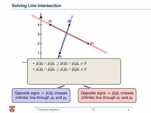
p̃1p2 ∩ p̃3p4 ⊇ p1p2 ∩ p̃3p4 6= ∅p̃1p2 ∩ p̃3p4 ⊇ p̃1p2 ∩ p3p4 6= ∅
Since p̃1p2 ∩ p̃3p4 consists of (at most) one point⇒ p1p2 ∩ p3p4 6= ∅
p1p2 crosses p3p4
p3
p4
(p3 − p1)× (p2 − p1) < 0
(p4 − p1)× (p2 − p1) < 0
p1p2 does not cross p3p4
7: Geometric Algorithms T.S. 8
Solving Line Intersection
x
y
1
2
3
4
1 2 3 4 5(0, 0)
p3
p4p2
p1
(p1 − p3)× (p4 − p3) = (3, 1)× (1, 3) = 8
(p2 − p3)× (p4 − p3) = (−1, 3)× (1, 3) = −6
Opposite signs ⇒ p1p2 crosses(infinite) line through p3 and p4
Opposite signs ⇒ p1p2 crosses(infinite) line through p3 and p4
(p3 − p1)× (p2 − p1) = (−3,−1)× (−4, 2) = −10
(p4 − p1)× (p2 − p1) = (−2, 2)× (−4, 2) = 4
Opposite signs ⇒ p3p4 crosses(infinite) line through p1 and p2
Opposite signs ⇒ p3p4 crosses(infinite) line through p1 and p2
p̃1p2 ∩ p̃3p4 ⊇ p1p2 ∩ p̃3p4 6= ∅p̃1p2 ∩ p̃3p4 ⊇ p̃1p2 ∩ p3p4 6= ∅Since p̃1p2 ∩ p̃3p4 consists of (at most) one point⇒ p1p2 ∩ p3p4 6= ∅
p1p2 crosses p3p4
p3
p4
(p3 − p1)× (p2 − p1) < 0
(p4 − p1)× (p2 − p1) < 0
p1p2 does not cross p3p4
7: Geometric Algorithms T.S. 8
Solving Line Intersection
x
y
1
2
3
4
1 2 3 4 5(0, 0)
p3
p4
p2
p1
(p1 − p3)× (p4 − p3) = (3, 1)× (1, 3) = 8
(p2 − p3)× (p4 − p3) = (−1, 3)× (1, 3) = −6
Opposite signs ⇒ p1p2 crosses(infinite) line through p3 and p4
Opposite signs ⇒ p1p2 crosses(infinite) line through p3 and p4
(p3 − p1)× (p2 − p1) = (−3,−1)× (−4, 2) = −10
(p4 − p1)× (p2 − p1) = (−2, 2)× (−4, 2) = 4
Opposite signs ⇒ p3p4 crosses(infinite) line through p1 and p2
Opposite signs ⇒ p3p4 crosses(infinite) line through p1 and p2
p̃1p2 ∩ p̃3p4 ⊇ p1p2 ∩ p̃3p4 6= ∅p̃1p2 ∩ p̃3p4 ⊇ p̃1p2 ∩ p3p4 6= ∅Since p̃1p2 ∩ p̃3p4 consists of (at most) one point⇒ p1p2 ∩ p3p4 6= ∅
p1p2 crosses p3p4
p3
p4
(p3 − p1)× (p2 − p1) < 0
(p4 − p1)× (p2 − p1) < 0
p1p2 does not cross p3p4
7: Geometric Algorithms T.S. 8
Solving Line Intersection
x
y
(0, 0)
p3
p4
p2
p1
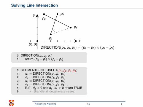
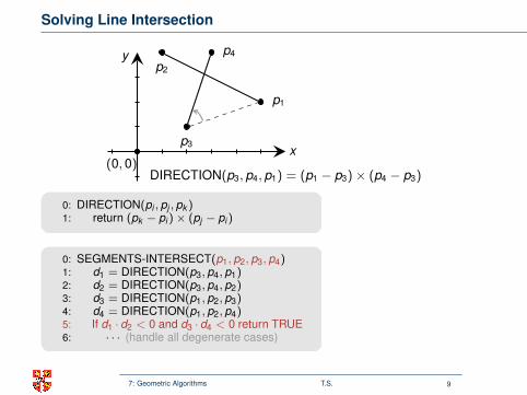
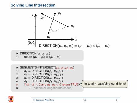
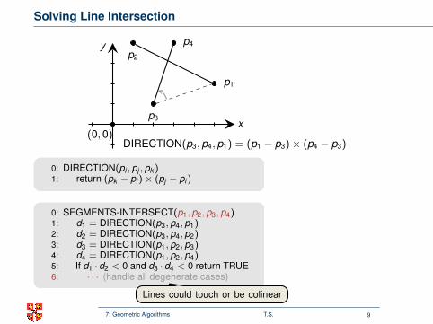
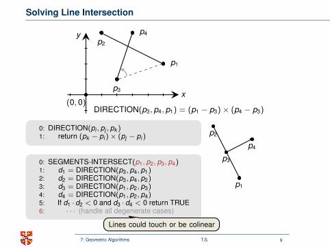
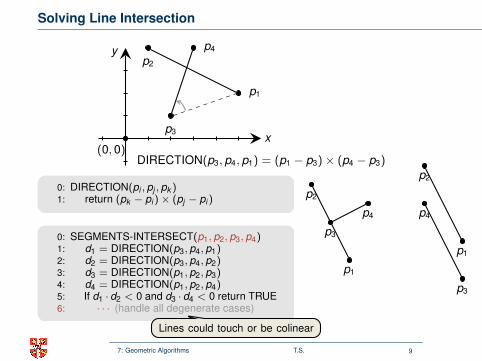
DIRECTION(p3, p4, p1) = (p1 − p3)× (p4 − p3)
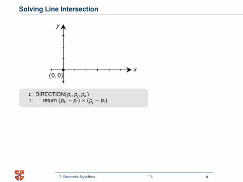
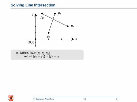
0: DIRECTION(pi , pj , pk )1: return (pk − pi )× (pj − pi )
0: SEGMENTS-INTERSECT(p1, p2, p3, p4)1: d1 = DIRECTION(p3, p4, p1)2: d2 = DIRECTION(p3, p4, p2)3: d3 = DIRECTION(p1, p2, p3)4: d4 = DIRECTION(p1, p2, p4)5: If d1 · d2 < 0 and d3 · d4 < 0 return TRUE6: · · · (handle all degenerate cases)
In total 4 satisfying conditions!
Lines could touch or be colinear
p2
p1
p3
p4
p2
p1
p4
p3
7: Geometric Algorithms T.S. 9
Solving Line Intersection
x
y
(0, 0)
p3
p4
p2
p1
DIRECTION(p3, p4, p1) = (p1 − p3)× (p4 − p3)
0: DIRECTION(pi , pj , pk )1: return (pk − pi )× (pj − pi )
0: SEGMENTS-INTERSECT(p1, p2, p3, p4)1: d1 = DIRECTION(p3, p4, p1)2: d2 = DIRECTION(p3, p4, p2)3: d3 = DIRECTION(p1, p2, p3)4: d4 = DIRECTION(p1, p2, p4)5: If d1 · d2 < 0 and d3 · d4 < 0 return TRUE6: · · · (handle all degenerate cases)
In total 4 satisfying conditions!
Lines could touch or be colinear
p2
p1
p3
p4
p2
p1
p4
p3
7: Geometric Algorithms T.S. 9
Outline
Introduction and Line Intersection
Convex Hull
Glimpse at (More) Advanced Algorithms
7: Geometric Algorithms T.S. 10
Convex Hull
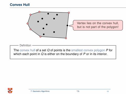
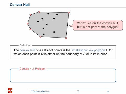
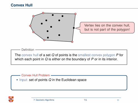
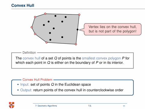
Vertex lies on the convex hull,but is not part of the polygon!
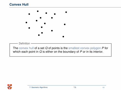
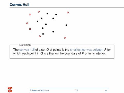
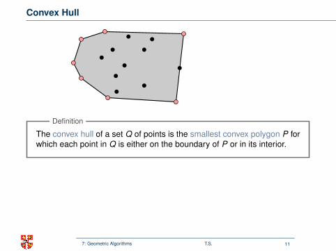
The convex hull of a set Q of points is the smallest convex polygon P forwhich each point in Q is either on the boundary of P or in its interior.
Definition
Smallest perimeter fence enclosing the points
Input: set of points Q in the Euclidean space
Output: return points of the convex hull in counterclockwise order
Convex Hull Problem
7: Geometric Algorithms T.S. 11
Convex Hull
Vertex lies on the convex hull,but is not part of the polygon!
The convex hull of a set Q of points is the smallest convex polygon P forwhich each point in Q is either on the boundary of P or in its interior.
Definition
Smallest perimeter fence enclosing the points
Input: set of points Q in the Euclidean space
Output: return points of the convex hull in counterclockwise order
Convex Hull Problem
7: Geometric Algorithms T.S. 11

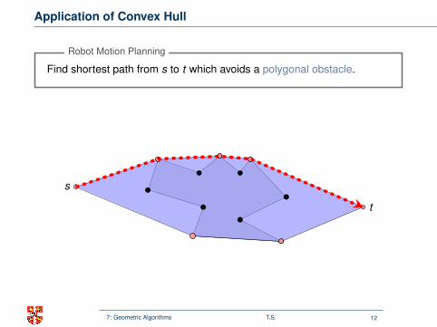
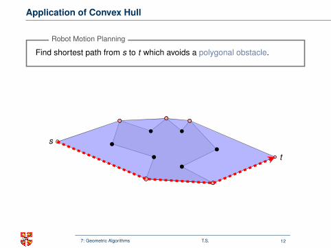
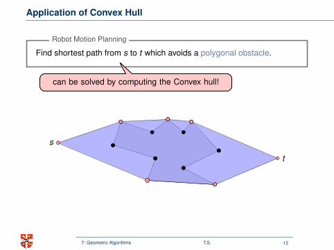
Application of Convex Hull
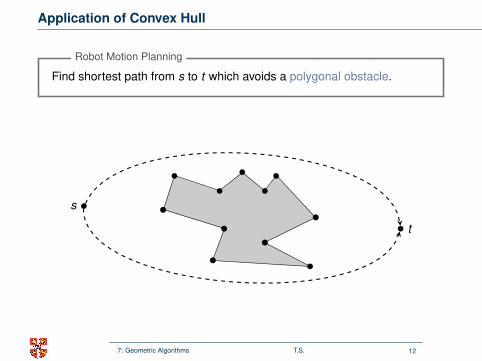
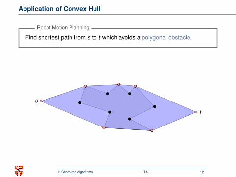
Find shortest path from s to t which avoids a polygonal obstacle.
Robot Motion Planning
can be solved by computing the Convex hull!
s
t
t
s
7: Geometric Algorithms T.S. 12
Application of Convex Hull
Find shortest path from s to t which avoids a polygonal obstacle.
Robot Motion Planning
can be solved by computing the Convex hull!
s
t
t
s
7: Geometric Algorithms T.S. 12

Application of Convex Hull
Find shortest path from s to t which avoids a polygonal obstacle.
Robot Motion Planning
can be solved by computing the Convex hull!
s
t
t
s
7: Geometric Algorithms T.S. 12

Application of Convex Hull
Find shortest path from s to t which avoids a polygonal obstacle.
Robot Motion Planning
can be solved by computing the Convex hull!
s
t
t
s
7: Geometric Algorithms T.S. 12
Application of Convex Hull
Find shortest path from s to t which avoids a polygonal obstacle.
Robot Motion Planning
can be solved by computing the Convex hull!
s
t
t
s
7: Geometric Algorithms T.S. 12
Application of Convex Hull
Find shortest path from s to t which avoids a polygonal obstacle.
Robot Motion Planning
can be solved by computing the Convex hull!
s
t
t
s
7: Geometric Algorithms T.S. 12
Application of Convex Hull
Find shortest path from s to t which avoids a polygonal obstacle.
Robot Motion Planning
can be solved by computing the Convex hull!
s
t
t
s
7: Geometric Algorithms T.S. 12
Application of Convex Hull
Find shortest path from s to t which avoids a polygonal obstacle.
Robot Motion Planning
can be solved by computing the Convex hull!
s
t
t
s
7: Geometric Algorithms T.S. 12
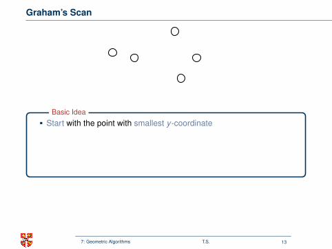
Graham’s Scan
00
1
2
34
x
y
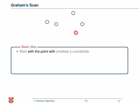
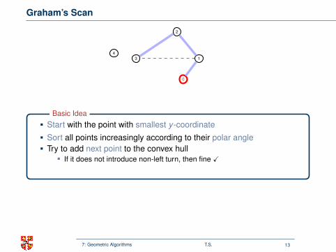
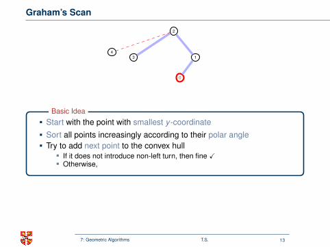
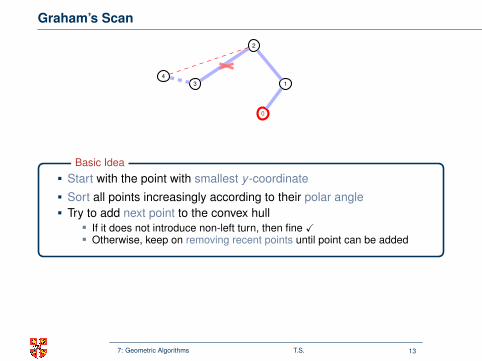
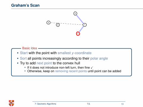
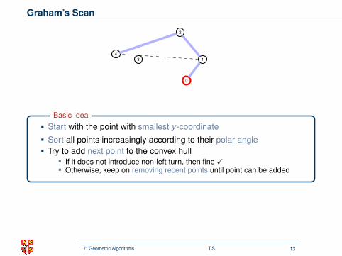
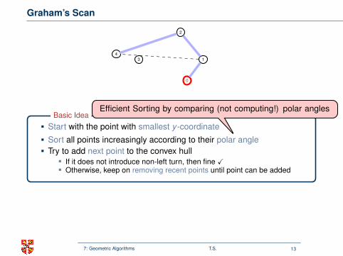
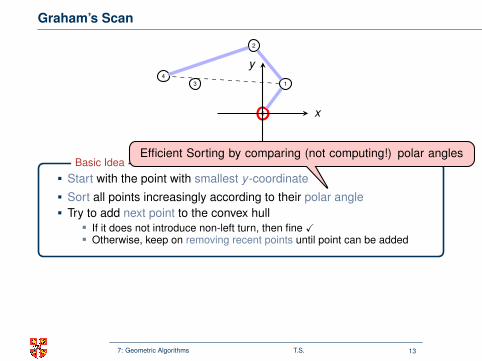
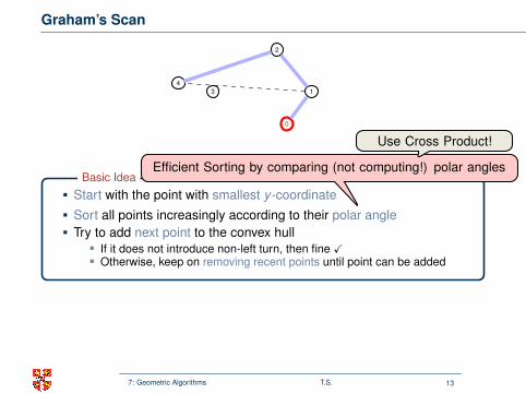
Start with the point with smallest y -coordinate
Sort all points increasingly according to their polar angleTry to add next point to the convex hull
If it does not introduce non-left turn, then fine
X
Otherwise,
keep on removing recent points until point can be added
Basic Idea
Efficient Sorting by comparing (not computing!) polar angles
Use Cross Product!
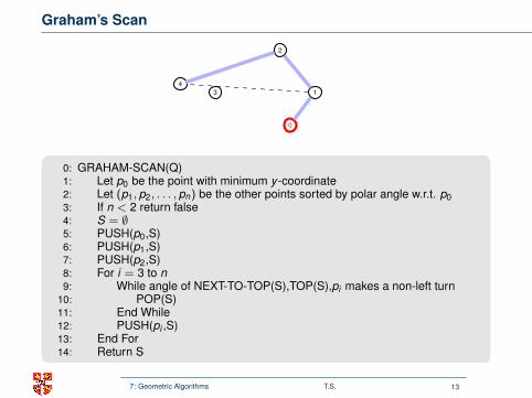
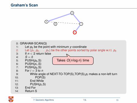
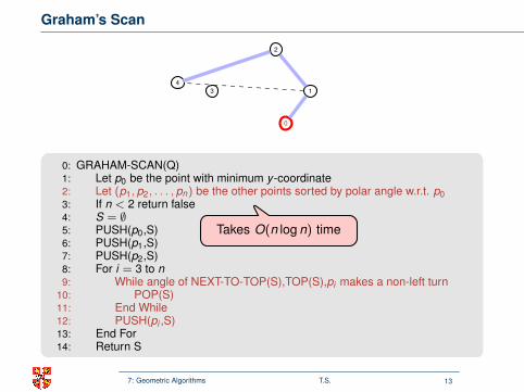
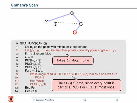
0: GRAHAM-SCAN(Q)1: Let p0 be the point with minimum y -coordinate2: Let (p1, p2, . . . , pn) be the other points sorted by polar angle w.r.t. p03: If n < 2 return false4: S = ∅5: PUSH(p0,S)6: PUSH(p1,S)7: PUSH(p2,S)8: For i = 3 to n9: While angle of NEXT-TO-TOP(S),TOP(S),pi makes a non-left turn
10: POP(S)11: End While12: PUSH(pi ,S)13: End For14: Return S
Takes O(n log n) time
Takes O(n) time, since every point ispart of a PUSH or POP at most once.
Overall Runtime: O(n log n)
7: Geometric Algorithms T.S. 13
Graham’s Scan
0
0
1
2
34
x
y
Start with the point with smallest y -coordinate
Sort all points increasingly according to their polar angleTry to add next point to the convex hull
If it does not introduce non-left turn, then fine
X
Otherwise,
keep on removing recent points until point can be added
Basic Idea
Efficient Sorting by comparing (not computing!) polar angles
Use Cross Product!
0: GRAHAM-SCAN(Q)1: Let p0 be the point with minimum y -coordinate2: Let (p1, p2, . . . , pn) be the other points sorted by polar angle w.r.t. p03: If n < 2 return false4: S = ∅5: PUSH(p0,S)6: PUSH(p1,S)7: PUSH(p2,S)8: For i = 3 to n9: While angle of NEXT-TO-TOP(S),TOP(S),pi makes a non-left turn
10: POP(S)11: End While12: PUSH(pi ,S)13: End For14: Return S
Takes O(n log n) time
Takes O(n) time, since every point ispart of a PUSH or POP at most once.
Overall Runtime: O(n log n)
7: Geometric Algorithms T.S. 13

Graham’s Scan
0
0
1
2
34
x
y
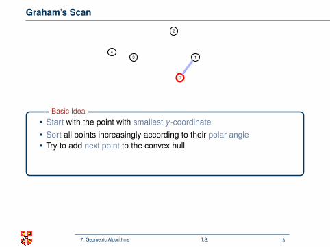
Start with the point with smallest y -coordinate
Sort all points increasingly according to their polar angle
Try to add next point to the convex hull
If it does not introduce non-left turn, then fine
X
Otherwise,
keep on removing recent points until point can be added
Basic Idea
Efficient Sorting by comparing (not computing!) polar angles
Use Cross Product!
0: GRAHAM-SCAN(Q)1: Let p0 be the point with minimum y -coordinate2: Let (p1, p2, . . . , pn) be the other points sorted by polar angle w.r.t. p03: If n < 2 return false4: S = ∅5: PUSH(p0,S)6: PUSH(p1,S)7: PUSH(p2,S)8: For i = 3 to n9: While angle of NEXT-TO-TOP(S),TOP(S),pi makes a non-left turn
10: POP(S)11: End While12: PUSH(pi ,S)13: End For14: Return S
Takes O(n log n) time
Takes O(n) time, since every point ispart of a PUSH or POP at most once.
Overall Runtime: O(n log n)
7: Geometric Algorithms T.S. 13

Graham’s Scan
0
0
1
2
34
x
y
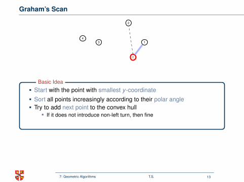
Start with the point with smallest y -coordinate
Sort all points increasingly according to their polar angleTry to add next point to the convex hull
If it does not introduce non-left turn, then fine
X
Otherwise,
keep on removing recent points until point can be added
Basic Idea
Efficient Sorting by comparing (not computing!) polar angles
Use Cross Product!
0: GRAHAM-SCAN(Q)1: Let p0 be the point with minimum y -coordinate2: Let (p1, p2, . . . , pn) be the other points sorted by polar angle w.r.t. p03: If n < 2 return false4: S = ∅5: PUSH(p0,S)6: PUSH(p1,S)7: PUSH(p2,S)8: For i = 3 to n9: While angle of NEXT-TO-TOP(S),TOP(S),pi makes a non-left turn
10: POP(S)11: End While12: PUSH(pi ,S)13: End For14: Return S
Takes O(n log n) time
Takes O(n) time, since every point ispart of a PUSH or POP at most once.
Overall Runtime: O(n log n)
7: Geometric Algorithms T.S. 13
Graham’s Scan
0
0
1
2
34
x
y
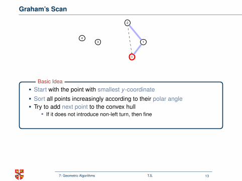
Start with the point with smallest y -coordinate
Sort all points increasingly according to their polar angleTry to add next point to the convex hull
If it does not introduce non-left turn, then fine
X
Otherwise,
keep on removing recent points until point can be added
Basic Idea
Efficient Sorting by comparing (not computing!) polar angles
Use Cross Product!
0: GRAHAM-SCAN(Q)1: Let p0 be the point with minimum y -coordinate2: Let (p1, p2, . . . , pn) be the other points sorted by polar angle w.r.t. p03: If n < 2 return false4: S = ∅5: PUSH(p0,S)6: PUSH(p1,S)7: PUSH(p2,S)8: For i = 3 to n9: While angle of NEXT-TO-TOP(S),TOP(S),pi makes a non-left turn
10: POP(S)11: End While12: PUSH(pi ,S)13: End For14: Return S
Takes O(n log n) time
Takes O(n) time, since every point ispart of a PUSH or POP at most once.
Overall Runtime: O(n log n)
7: Geometric Algorithms T.S. 13
Graham’s Scan
0
0
1
2
34
x
y
Start with the point with smallest y -coordinate
Sort all points increasingly according to their polar angleTry to add next point to the convex hull
If it does not introduce non-left turn, then fine
XOtherwise,
keep on removing recent points until point can be added
Basic Idea
Efficient Sorting by comparing (not computing!) polar angles
Use Cross Product!
0: GRAHAM-SCAN(Q)1: Let p0 be the point with minimum y -coordinate2: Let (p1, p2, . . . , pn) be the other points sorted by polar angle w.r.t. p03: If n < 2 return false4: S = ∅5: PUSH(p0,S)6: PUSH(p1,S)7: PUSH(p2,S)8: For i = 3 to n9: While angle of NEXT-TO-TOP(S),TOP(S),pi makes a non-left turn
10: POP(S)11: End While12: PUSH(pi ,S)13: End For14: Return S
Takes O(n log n) time
Takes O(n) time, since every point ispart of a PUSH or POP at most once.
Overall Runtime: O(n log n)
7: Geometric Algorithms T.S. 13
Graham’s Scan
0
0
1
2
34
x
y
Start with the point with smallest y -coordinate
Sort all points increasingly according to their polar angleTry to add next point to the convex hull
If it does not introduce non-left turn, then fine X
Otherwise,
keep on removing recent points until point can be added
Basic Idea
Efficient Sorting by comparing (not computing!) polar angles
Use Cross Product!
0: GRAHAM-SCAN(Q)1: Let p0 be the point with minimum y -coordinate2: Let (p1, p2, . . . , pn) be the other points sorted by polar angle w.r.t. p03: If n < 2 return false4: S = ∅5: PUSH(p0,S)6: PUSH(p1,S)7: PUSH(p2,S)8: For i = 3 to n9: While angle of NEXT-TO-TOP(S),TOP(S),pi makes a non-left turn
10: POP(S)11: End While12: PUSH(pi ,S)13: End For14: Return S
Takes O(n log n) time
Takes O(n) time, since every point ispart of a PUSH or POP at most once.
Overall Runtime: O(n log n)
7: Geometric Algorithms T.S. 13
Graham’s Scan
0
0
1
2
34
x
y
Start with the point with smallest y -coordinate
Sort all points increasingly according to their polar angleTry to add next point to the convex hull
If it does not introduce non-left turn, then fine XOtherwise,
keep on removing recent points until point can be added
Basic Idea
Efficient Sorting by comparing (not computing!) polar angles
Use Cross Product!
0: GRAHAM-SCAN(Q)1: Let p0 be the point with minimum y -coordinate2: Let (p1, p2, . . . , pn) be the other points sorted by polar angle w.r.t. p03: If n < 2 return false4: S = ∅5: PUSH(p0,S)6: PUSH(p1,S)7: PUSH(p2,S)8: For i = 3 to n9: While angle of NEXT-TO-TOP(S),TOP(S),pi makes a non-left turn
10: POP(S)11: End While12: PUSH(pi ,S)13: End For14: Return S
Takes O(n log n) time
Takes O(n) time, since every point ispart of a PUSH or POP at most once.
Overall Runtime: O(n log n)
7: Geometric Algorithms T.S. 13

Graham’s Scan
0
0
1
2
34
x
y
Start with the point with smallest y -coordinate
Sort all points increasingly according to their polar angleTry to add next point to the convex hull
If it does not introduce non-left turn, then fine XOtherwise, keep on removing recent points until point can be added
Basic Idea
Efficient Sorting by comparing (not computing!) polar angles
Use Cross Product!
0: GRAHAM-SCAN(Q)1: Let p0 be the point with minimum y -coordinate2: Let (p1, p2, . . . , pn) be the other points sorted by polar angle w.r.t. p03: If n < 2 return false4: S = ∅5: PUSH(p0,S)6: PUSH(p1,S)7: PUSH(p2,S)8: For i = 3 to n9: While angle of NEXT-TO-TOP(S),TOP(S),pi makes a non-left turn
10: POP(S)11: End While12: PUSH(pi ,S)13: End For14: Return S
Takes O(n log n) time
Takes O(n) time, since every point ispart of a PUSH or POP at most once.
Overall Runtime: O(n log n)
7: Geometric Algorithms T.S. 13
Graham’s Scan
0
0
1
2
34
x
y
Start with the point with smallest y -coordinate
Sort all points increasingly according to their polar angleTry to add next point to the convex hull
If it does not introduce non-left turn, then fine XOtherwise, keep on removing recent points until point can be added
Basic IdeaEfficient Sorting by comparing (not computing!) polar angles
Use Cross Product!
0: GRAHAM-SCAN(Q)1: Let p0 be the point with minimum y -coordinate2: Let (p1, p2, . . . , pn) be the other points sorted by polar angle w.r.t. p03: If n < 2 return false4: S = ∅5: PUSH(p0,S)6: PUSH(p1,S)7: PUSH(p2,S)8: For i = 3 to n9: While angle of NEXT-TO-TOP(S),TOP(S),pi makes a non-left turn
10: POP(S)11: End While12: PUSH(pi ,S)13: End For14: Return S
Takes O(n log n) time
Takes O(n) time, since every point ispart of a PUSH or POP at most once.
Overall Runtime: O(n log n)
7: Geometric Algorithms T.S. 13
Graham’s Scan
0
0
1
2
34
x
y
0: GRAHAM-SCAN(Q)1: Let p0 be the point with minimum y -coordinate2: Let (p1, p2, . . . , pn) be the other points sorted by polar angle w.r.t. p03: If n < 2 return false4: S = ∅5: PUSH(p0,S)6: PUSH(p1,S)7: PUSH(p2,S)8: For i = 3 to n9: While angle of NEXT-TO-TOP(S),TOP(S),pi makes a non-left turn
10: POP(S)11: End While12: PUSH(pi ,S)13: End For14: Return S
Takes O(n log n) time
Takes O(n) time, since every point ispart of a PUSH or POP at most once.
Overall Runtime: O(n log n)
7: Geometric Algorithms T.S. 13
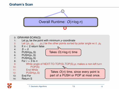
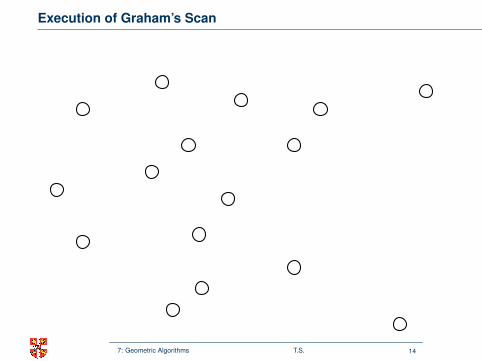
Execution of Graham’s Scan
0
7
10
1
2
3
4
6
5
8
12
9
1311
14
15
i = 0123456789101112131415 X 0 1 2 345 6 78 9 101112 13 1415
7: Geometric Algorithms T.S. 14
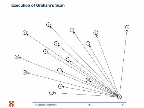
Execution of Graham’s Scan
0
7
10
1
2
3
4
6
5
8
12
9
1311
14
15
i = 0123456789101112131415 X 0 1 2 345 6 78 9 101112 13 1415
7: Geometric Algorithms T.S. 14
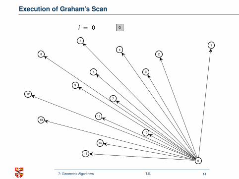
Execution of Graham’s Scan
0
7
10
1
2
3
4
6
5
8
12
9
1311
14
15
i = 0
123456789101112131415 X
0
1 2 345 6 78 9 101112 13 1415
7: Geometric Algorithms T.S. 14
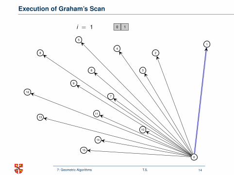
Execution of Graham’s Scan
0
7
10
1
2
3
4
6
5
8
12
9
1311
14
15
i =
0
1
23456789101112131415 X
0 1
2 345 6 78 9 101112 13 1415
7: Geometric Algorithms T.S. 14
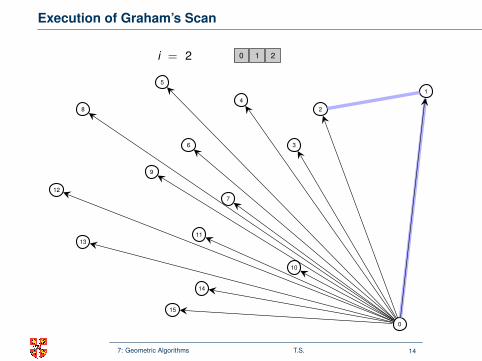
Execution of Graham’s Scan
0
7
10
1
2
3
4
6
5
8
12
9
1311
14
15
i =
01
2
3456789101112131415 X
0 1 2
345 6 78 9 101112 13 1415
7: Geometric Algorithms T.S. 14
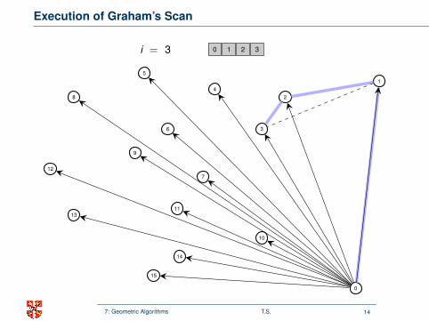
Execution of Graham’s Scan
0
7
10
1
2
3
4
6
5
8
12
9
1311
14
15
i =
012
3
456789101112131415 X
0 1 2 3
45 6 78 9 101112 13 1415
7: Geometric Algorithms T.S. 14
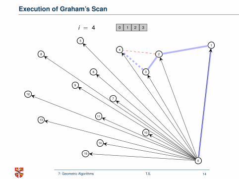
Execution of Graham’s Scan
0
7
10
1
2
3
4
6
5
8
12
9
1311
14
15
i =
0123
4
56789101112131415 X
0 1 2 3
45 6 78 9 101112 13 1415
7: Geometric Algorithms T.S. 14
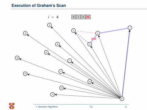
Execution of Graham’s Scan
0
7
10
1
2
3
4
6
5
8
12
9
1311
14
15
i =
0123
4
56789101112131415 X
0 1 2 3
45 6 78 9 101112 13 1415
7: Geometric Algorithms T.S. 14

Execution of Graham’s Scan
0
7
10
1
2
3
4
6
5
8
12
9
1311
14
15
i =
0123
4
56789101112131415 X
0 1 2
345 6 78 9 101112 13 1415
7: Geometric Algorithms T.S. 14
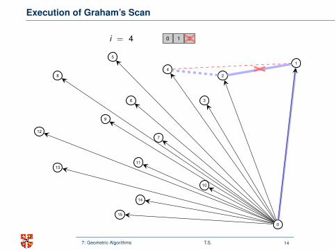
Execution of Graham’s Scan
0
7
10
1
2
3
4
6
5
8
12
9
1311
14
15
i =
0123
4
56789101112131415 X
0 1 2
345 6 78 9 101112 13 1415
7: Geometric Algorithms T.S. 14

Execution of Graham’s Scan
0
7
10
1
2
3
4
6
5
8
12
9
1311
14
15
i =
0123
4
56789101112131415 X
0 1
2 3
4
5 6 78 9 101112 13 1415
7: Geometric Algorithms T.S. 14

Execution of Graham’s Scan
0
7
10
1
2
3
4
6
5
8
12
9
1311
14
15
i =
01234
5
6789101112131415 X
0 1
2 3
4
5 6 78 9 101112 13 1415
7: Geometric Algorithms T.S. 14

Execution of Graham’s Scan
0
7
10
1
2
3
4
6
5
8
12
9
1311
14
15
i =
01234
5
6789101112131415 X
0 1
2 3
4
5 6 78 9 101112 13 1415
7: Geometric Algorithms T.S. 14
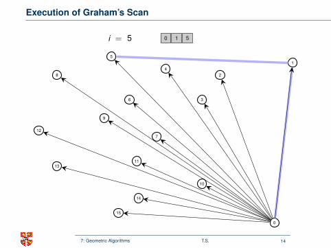
Execution of Graham’s Scan
0
7
10
1
2
3
4
6
5
8
12
9
1311
14
15
i =
01234
5
6789101112131415 X
0 1
2 34
5
6 78 9 101112 13 1415
7: Geometric Algorithms T.S. 14
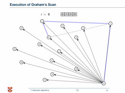
Execution of Graham’s Scan
0
7
10
1
2
3
4
6
5
8
12
9
1311
14
15
i =
012345
6
789101112131415 X
0 1
2 34
5 6
78 9 101112 13 1415
7: Geometric Algorithms T.S. 14
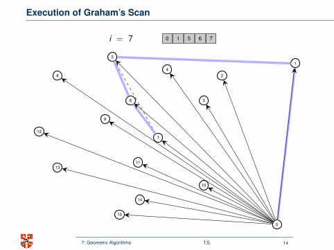
Execution of Graham’s Scan
0
7
10
1
2
3
4
6
5
8
12
9
1311
14
15
i =
0123456
7
89101112131415 X
0 1
2 34
5 6 7
8 9 101112 13 1415
7: Geometric Algorithms T.S. 14
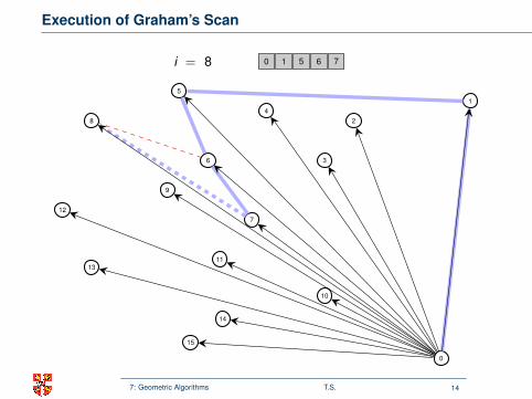
Execution of Graham’s Scan
0
7
10
1
2
3
4
6
5
8
12
9
1311
14
15
i =
01234567
8
9101112131415 X
0 1
2 34
5 6 7
8 9 101112 13 1415
7: Geometric Algorithms T.S. 14
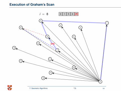
Execution of Graham’s Scan
0
7
10
1
2
3
4
6
5
8
12
9
1311
14
15
i =
01234567
8
9101112131415 X
0 1
2 34
5 6 7
8 9 101112 13 1415
7: Geometric Algorithms T.S. 14
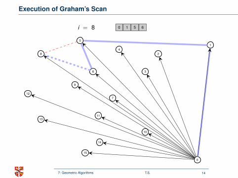
Execution of Graham’s Scan
0
7
10
1
2
3
4
6
5
8
12
9
1311
14
15
i =
01234567
8
9101112131415 X
0 1
2 34
5 6
78 9 101112 13 1415
7: Geometric Algorithms T.S. 14
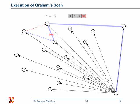
Execution of Graham’s Scan
0
7
10
1
2
3
4
6
5
8
12
9
1311
14
15
i =
01234567
8
9101112131415 X
0 1
2 34
5 6
78 9 101112 13 1415
7: Geometric Algorithms T.S. 14
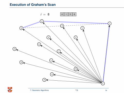
Execution of Graham’s Scan
0
7
10
1
2
3
4
6
5
8
12
9
1311
14
15
i =
01234567
8
9101112131415 X
0 1
2 34
5
6 7
8
9 101112 13 1415
7: Geometric Algorithms T.S. 14

Execution of Graham’s Scan
0
7
10
1
2
3
4
6
5
8
12
9
1311
14
15
i =
012345678
9
101112131415 X
0 1
2 34
5
6 7
8 9
101112 13 1415
7: Geometric Algorithms T.S. 14
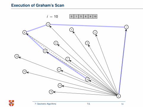
Execution of Graham’s Scan
0
7
10
1
2
3
4
6
5
8
12
9
1311
14
15
i =
0123456789
10
1112131415 X
0 1
2 34
5
6 7
8 9 10
1112 13 1415
7: Geometric Algorithms T.S. 14

Execution of Graham’s Scan
0
7
10
1
2
3
4
6
5
8
12
9
1311
14
15
i =
012345678910
11
12131415 X
0 1
2 34
5
6 7
8 9 10
1112 13 1415
7: Geometric Algorithms T.S. 14
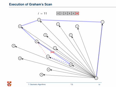
Execution of Graham’s Scan
0
7
10
1
2
3
4
6
5
8
12
9
1311
14
15
i =
012345678910
11
12131415 X
0 1
2 34
5
6 7
8 9 10
1112 13 1415
7: Geometric Algorithms T.S. 14
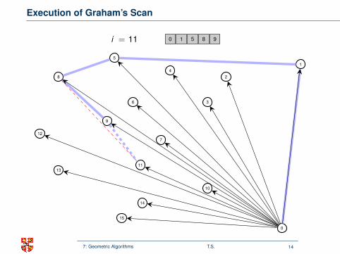
Execution of Graham’s Scan
0
7
10
1
2
3
4
6
5
8
12
9
1311
14
15
i =
012345678910
11
12131415 X
0 1
2 34
5
6 7
8 9
101112 13 1415
7: Geometric Algorithms T.S. 14
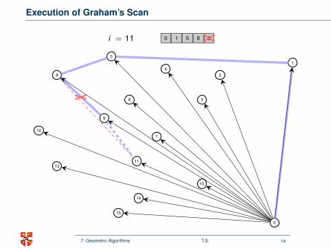
Execution of Graham’s Scan
0
7
10
1
2
3
4
6
5
8
12
9
1311
14
15
i =
012345678910
11
12131415 X
0 1
2 34
5
6 7
8 9
101112 13 1415
7: Geometric Algorithms T.S. 14
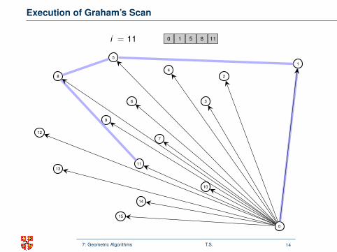
Execution of Graham’s Scan
0
7
10
1
2
3
4
6
5
8
12
9
1311
14
15
i =
012345678910
11
12131415 X
0 1
2 34
5
6 7
8
9 10
11
12 13 1415
7: Geometric Algorithms T.S. 14
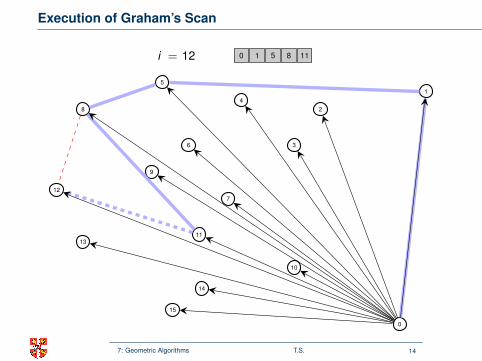
Execution of Graham’s Scan
0
7
10
1
2
3
4
6
5
8
12
9
1311
14
15
i =
01234567891011
12
131415 X
0 1
2 34
5
6 7
8
9 10
11
12 13 1415
7: Geometric Algorithms T.S. 14
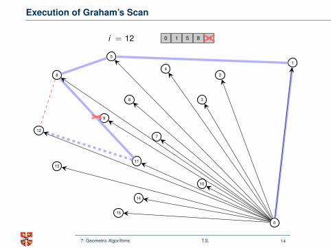
Execution of Graham’s Scan
0
7
10
1
2
3
4
6
5
8
12
9
1311
14
15
i =
01234567891011
12
131415 X
0 1
2 34
5
6 7
8
9 10
11
12 13 1415
7: Geometric Algorithms T.S. 14
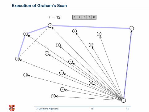
Execution of Graham’s Scan
0
7
10
1
2
3
4
6
5
8
12
9
1311
14
15
i =
01234567891011
12
131415 X
0 1
2 34
5
6 7
8
9 1011
12
13 1415
7: Geometric Algorithms T.S. 14
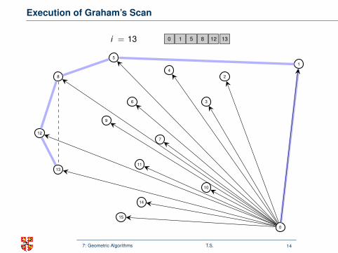
Execution of Graham’s Scan
0
7
10
1
2
3
4
6
5
8
12
9
1311
14
15
i =
0123456789101112
13
1415 X
0 1
2 34
5
6 7
8
9 1011
12 13
1415
7: Geometric Algorithms T.S. 14
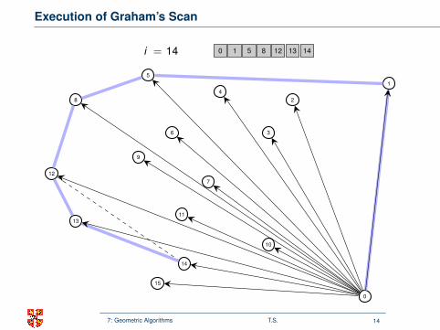
Execution of Graham’s Scan
0
7
10
1
2
3
4
6
5
8
12
9
1311
14
15
i =
012345678910111213
14
15 X
0 1
2 34
5
6 7
8
9 1011
12 13 14
15
7: Geometric Algorithms T.S. 14
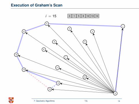
Execution of Graham’s Scan
0
7
10
1
2
3
4
6
5
8
12
9
1311
14
15
i =
01234567891011121314
15
X
0 1
2 34
5
6 7
8
9 1011
12 13 14
15
7: Geometric Algorithms T.S. 14
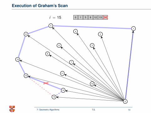
Execution of Graham’s Scan
0
7
10
1
2
3
4
6
5
8
12
9
1311
14
15
i =
01234567891011121314
15
X
0 1
2 34
5
6 7
8
9 1011
12 13 14
15
7: Geometric Algorithms T.S. 14
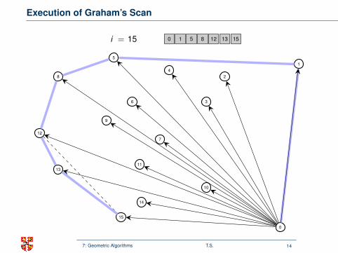
Execution of Graham’s Scan
0
7
10
1
2
3
4
6
5
8
12
9
1311
14
15
i =
01234567891011121314
15
X
0 1
2 34
5
6 7
8
9 1011
12 13
14
15
7: Geometric Algorithms T.S. 14
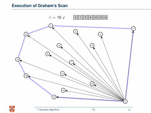
Execution of Graham’s Scan
0
7
10
1
2
3
4
6
5
8
12
9
1311
14
15
i =
01234567891011121314
15 X 0 1
2 34
5
6 7
8
9 1011
12 13
14
15
7: Geometric Algorithms T.S. 14
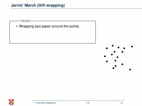
Jarvis’ March (Gift wrapping)
Wrapping taut paper around the points
1. Tape end of paper at lowest point2. Pull paper to the right until it touches a point3. Tape paper and go to 2
Intuition
1. Let p0 be the lowest point
2. Next point the one with smallest angle w.r.t. p0
3. Continue until highest point pk
4. Next point the one with smallest angle w.r.t. pk
5. Continue until p0 is reached
Algorithm
Here, we rotate the coordinate system by 180!
Runtime: O(n · h), where his no. points on convex hull.
Output sensitive algorithm!
7: Geometric Algorithms T.S. 15

Jarvis’ March (Gift wrapping)
Wrapping taut paper around the points1. Tape end of paper at lowest point
2. Pull paper to the right until it touches a point3. Tape paper and go to 2
Intuition
1. Let p0 be the lowest point
2. Next point the one with smallest angle w.r.t. p0
3. Continue until highest point pk
4. Next point the one with smallest angle w.r.t. pk
5. Continue until p0 is reached
Algorithm
Here, we rotate the coordinate system by 180!
Runtime: O(n · h), where his no. points on convex hull.
Output sensitive algorithm!
7: Geometric Algorithms T.S. 15
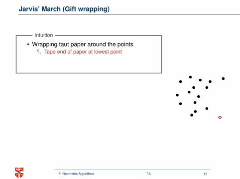
Jarvis’ March (Gift wrapping)
Wrapping taut paper around the points1. Tape end of paper at lowest point
2. Pull paper to the right until it touches a point3. Tape paper and go to 2
Intuition
1. Let p0 be the lowest point
2. Next point the one with smallest angle w.r.t. p0
3. Continue until highest point pk
4. Next point the one with smallest angle w.r.t. pk
5. Continue until p0 is reached
Algorithm
Here, we rotate the coordinate system by 180!
Runtime: O(n · h), where his no. points on convex hull.
Output sensitive algorithm!
7: Geometric Algorithms T.S. 15
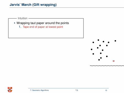
Jarvis’ March (Gift wrapping)
Wrapping taut paper around the points1. Tape end of paper at lowest point
2. Pull paper to the right until it touches a point3. Tape paper and go to 2
Intuition
1. Let p0 be the lowest point
2. Next point the one with smallest angle w.r.t. p0
3. Continue until highest point pk
4. Next point the one with smallest angle w.r.t. pk
5. Continue until p0 is reached
Algorithm
Here, we rotate the coordinate system by 180!
Runtime: O(n · h), where his no. points on convex hull.
Output sensitive algorithm!
7: Geometric Algorithms T.S. 15
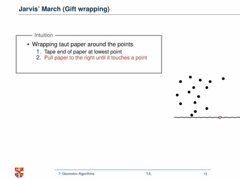
Jarvis’ March (Gift wrapping)
Wrapping taut paper around the points1. Tape end of paper at lowest point2. Pull paper to the right until it touches a point
3. Tape paper and go to 2
Intuition
1. Let p0 be the lowest point
2. Next point the one with smallest angle w.r.t. p0
3. Continue until highest point pk
4. Next point the one with smallest angle w.r.t. pk
5. Continue until p0 is reached
Algorithm
Here, we rotate the coordinate system by 180!
Runtime: O(n · h), where his no. points on convex hull.
Output sensitive algorithm!
7: Geometric Algorithms T.S. 15
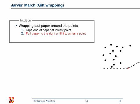
Jarvis’ March (Gift wrapping)
Wrapping taut paper around the points1. Tape end of paper at lowest point2. Pull paper to the right until it touches a point
3. Tape paper and go to 2
Intuition
1. Let p0 be the lowest point
2. Next point the one with smallest angle w.r.t. p0
3. Continue until highest point pk
4. Next point the one with smallest angle w.r.t. pk
5. Continue until p0 is reached
Algorithm
Here, we rotate the coordinate system by 180!
Runtime: O(n · h), where his no. points on convex hull.
Output sensitive algorithm!
7: Geometric Algorithms T.S. 15
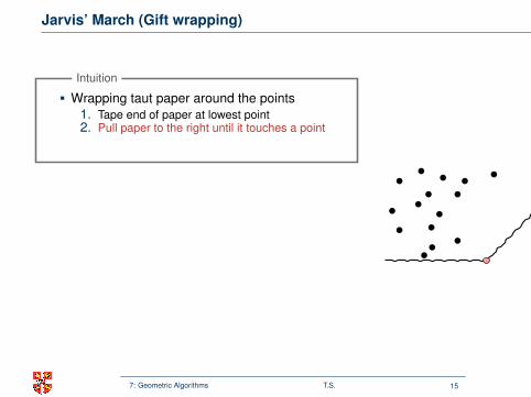
Jarvis’ March (Gift wrapping)
Wrapping taut paper around the points1. Tape end of paper at lowest point2. Pull paper to the right until it touches a point
3. Tape paper and go to 2
Intuition
1. Let p0 be the lowest point
2. Next point the one with smallest angle w.r.t. p0
3. Continue until highest point pk
4. Next point the one with smallest angle w.r.t. pk
5. Continue until p0 is reached
Algorithm
Here, we rotate the coordinate system by 180!
Runtime: O(n · h), where his no. points on convex hull.
Output sensitive algorithm!
7: Geometric Algorithms T.S. 15
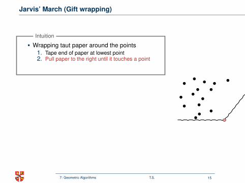
Jarvis’ March (Gift wrapping)
Wrapping taut paper around the points1. Tape end of paper at lowest point2. Pull paper to the right until it touches a point
3. Tape paper and go to 2
Intuition
1. Let p0 be the lowest point
2. Next point the one with smallest angle w.r.t. p0
3. Continue until highest point pk
4. Next point the one with smallest angle w.r.t. pk
5. Continue until p0 is reached
Algorithm
Here, we rotate the coordinate system by 180!
Runtime: O(n · h), where his no. points on convex hull.
Output sensitive algorithm!
7: Geometric Algorithms T.S. 15
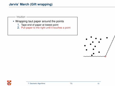
Jarvis’ March (Gift wrapping)
Wrapping taut paper around the points1. Tape end of paper at lowest point2. Pull paper to the right until it touches a point
3. Tape paper and go to 2
Intuition
1. Let p0 be the lowest point
2. Next point the one with smallest angle w.r.t. p0
3. Continue until highest point pk
4. Next point the one with smallest angle w.r.t. pk
5. Continue until p0 is reached
Algorithm
Here, we rotate the coordinate system by 180!
Runtime: O(n · h), where his no. points on convex hull.
Output sensitive algorithm!
7: Geometric Algorithms T.S. 15
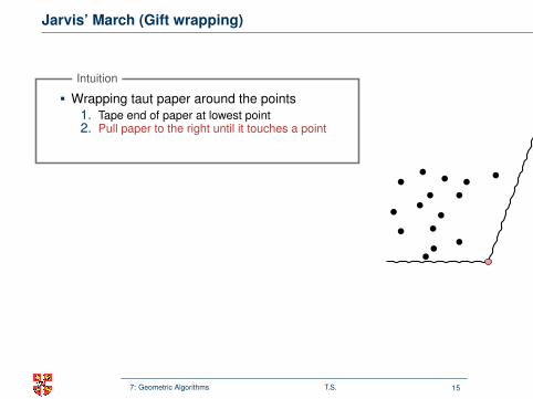
Jarvis’ March (Gift wrapping)
Wrapping taut paper around the points1. Tape end of paper at lowest point2. Pull paper to the right until it touches a point
3. Tape paper and go to 2
Intuition
1. Let p0 be the lowest point
2. Next point the one with smallest angle w.r.t. p0
3. Continue until highest point pk
4. Next point the one with smallest angle w.r.t. pk
5. Continue until p0 is reached
Algorithm
Here, we rotate the coordinate system by 180!
Runtime: O(n · h), where his no. points on convex hull.
Output sensitive algorithm!
7: Geometric Algorithms T.S. 15
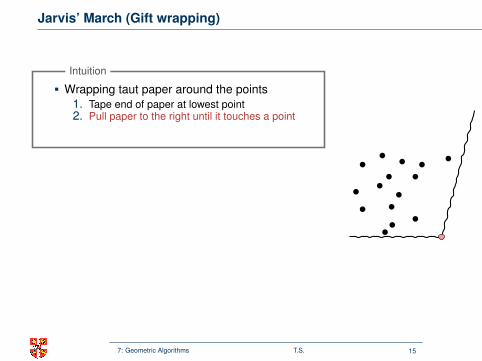
Jarvis’ March (Gift wrapping)
Wrapping taut paper around the points1. Tape end of paper at lowest point2. Pull paper to the right until it touches a point
3. Tape paper and go to 2
Intuition
1. Let p0 be the lowest point
2. Next point the one with smallest angle w.r.t. p0
3. Continue until highest point pk
4. Next point the one with smallest angle w.r.t. pk
5. Continue until p0 is reached
Algorithm
Here, we rotate the coordinate system by 180!
Runtime: O(n · h), where his no. points on convex hull.
Output sensitive algorithm!
7: Geometric Algorithms T.S. 15
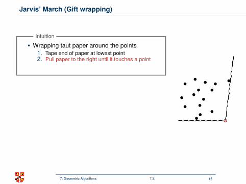
Jarvis’ March (Gift wrapping)
Wrapping taut paper around the points1. Tape end of paper at lowest point2. Pull paper to the right until it touches a point
3. Tape paper and go to 2
Intuition
1. Let p0 be the lowest point
2. Next point the one with smallest angle w.r.t. p0
3. Continue until highest point pk
4. Next point the one with smallest angle w.r.t. pk
5. Continue until p0 is reached
Algorithm
Here, we rotate the coordinate system by 180!
Runtime: O(n · h), where his no. points on convex hull.
Output sensitive algorithm!
7: Geometric Algorithms T.S. 15
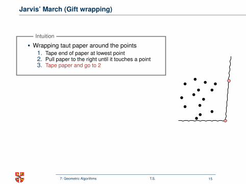
Jarvis’ March (Gift wrapping)
Wrapping taut paper around the points1. Tape end of paper at lowest point2. Pull paper to the right until it touches a point3. Tape paper and go to 2
Intuition
1. Let p0 be the lowest point
2. Next point the one with smallest angle w.r.t. p0
3. Continue until highest point pk
4. Next point the one with smallest angle w.r.t. pk
5. Continue until p0 is reached
Algorithm
Here, we rotate the coordinate system by 180!
Runtime: O(n · h), where his no. points on convex hull.
Output sensitive algorithm!
7: Geometric Algorithms T.S. 15
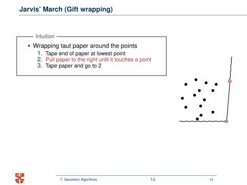
Jarvis’ March (Gift wrapping)
Wrapping taut paper around the points1. Tape end of paper at lowest point2. Pull paper to the right until it touches a point3. Tape paper and go to 2
Intuition
1. Let p0 be the lowest point
2. Next point the one with smallest angle w.r.t. p0
3. Continue until highest point pk
4. Next point the one with smallest angle w.r.t. pk
5. Continue until p0 is reached
Algorithm
Here, we rotate the coordinate system by 180!
Runtime: O(n · h), where his no. points on convex hull.
Output sensitive algorithm!
7: Geometric Algorithms T.S. 15
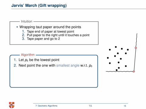
Jarvis’ March (Gift wrapping)
Wrapping taut paper around the points1. Tape end of paper at lowest point2. Pull paper to the right until it touches a point3. Tape paper and go to 2
Intuition
1. Let p0 be the lowest point
2. Next point the one with smallest angle w.r.t. p0
3. Continue until highest point pk
4. Next point the one with smallest angle w.r.t. pk
5. Continue until p0 is reached
Algorithm
Here, we rotate the coordinate system by 180!
Runtime: O(n · h), where his no. points on convex hull.
Output sensitive algorithm!
7: Geometric Algorithms T.S. 15
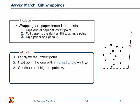
Jarvis’ March (Gift wrapping)
Wrapping taut paper around the points1. Tape end of paper at lowest point2. Pull paper to the right until it touches a point3. Tape paper and go to 2
Intuition
1. Let p0 be the lowest point
2. Next point the one with smallest angle w.r.t. p0
3. Continue until highest point pk
4. Next point the one with smallest angle w.r.t. pk
5. Continue until p0 is reached
Algorithm
Here, we rotate the coordinate system by 180!
Runtime: O(n · h), where his no. points on convex hull.
Output sensitive algorithm!
7: Geometric Algorithms T.S. 15
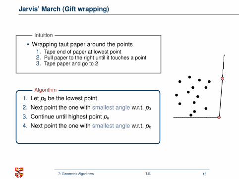
Jarvis’ March (Gift wrapping)
Wrapping taut paper around the points1. Tape end of paper at lowest point2. Pull paper to the right until it touches a point3. Tape paper and go to 2
Intuition
1. Let p0 be the lowest point
2. Next point the one with smallest angle w.r.t. p0
3. Continue until highest point pk
4. Next point the one with smallest angle w.r.t. pk
5. Continue until p0 is reached
Algorithm
Here, we rotate the coordinate system by 180!
Runtime: O(n · h), where his no. points on convex hull.
Output sensitive algorithm!
7: Geometric Algorithms T.S. 15
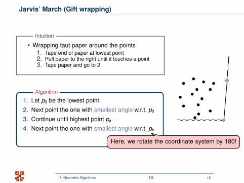
Jarvis’ March (Gift wrapping)
Wrapping taut paper around the points1. Tape end of paper at lowest point2. Pull paper to the right until it touches a point3. Tape paper and go to 2
Intuition
1. Let p0 be the lowest point
2. Next point the one with smallest angle w.r.t. p0
3. Continue until highest point pk
4. Next point the one with smallest angle w.r.t. pk
5. Continue until p0 is reached
Algorithm
Here, we rotate the coordinate system by 180!
Runtime: O(n · h), where his no. points on convex hull.
Output sensitive algorithm!
7: Geometric Algorithms T.S. 15
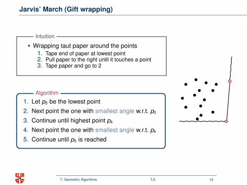
Jarvis’ March (Gift wrapping)
Wrapping taut paper around the points1. Tape end of paper at lowest point2. Pull paper to the right until it touches a point3. Tape paper and go to 2
Intuition
1. Let p0 be the lowest point
2. Next point the one with smallest angle w.r.t. p0
3. Continue until highest point pk
4. Next point the one with smallest angle w.r.t. pk
5. Continue until p0 is reached
Algorithm
Here, we rotate the coordinate system by 180!
Runtime: O(n · h), where his no. points on convex hull.
Output sensitive algorithm!
7: Geometric Algorithms T.S. 15
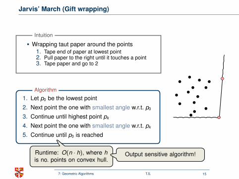
Jarvis’ March (Gift wrapping)
Wrapping taut paper around the points1. Tape end of paper at lowest point2. Pull paper to the right until it touches a point3. Tape paper and go to 2
Intuition
1. Let p0 be the lowest point
2. Next point the one with smallest angle w.r.t. p0
3. Continue until highest point pk
4. Next point the one with smallest angle w.r.t. pk
5. Continue until p0 is reached
Algorithm
Here, we rotate the coordinate system by 180!
Runtime: O(n · h), where his no. points on convex hull.
Output sensitive algorithm!
7: Geometric Algorithms T.S. 15
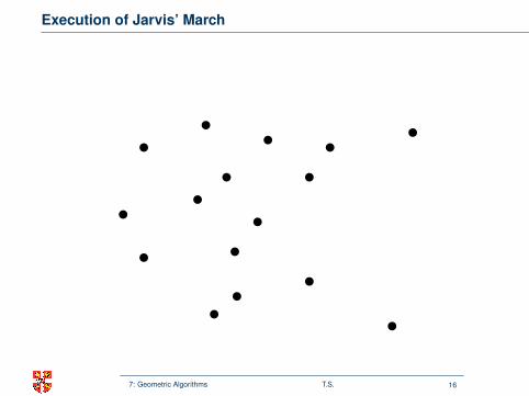
Execution of Jarvis’ March
x
y
x
y
x
y
x
y
x
y
x
y
x
y
7: Geometric Algorithms T.S. 16
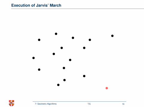
Execution of Jarvis’ March
x
y
x
y
x
y
x
y
x
y
x
y
x
y
7: Geometric Algorithms T.S. 16

Execution of Jarvis’ March
x
y
x
y
x
y
x
y
x
y
x
y
x
y
7: Geometric Algorithms T.S. 16

Execution of Jarvis’ March
x
y
x
y
x
y
x
y
x
y
x
y
x
y
7: Geometric Algorithms T.S. 16

Execution of Jarvis’ March
x
y
x
y
x
y
x
y
x
y
x
y
x
y
7: Geometric Algorithms T.S. 16

Execution of Jarvis’ March
x
y
x
y
x
y
x
y
x
y
x
y
x
y
7: Geometric Algorithms T.S. 16
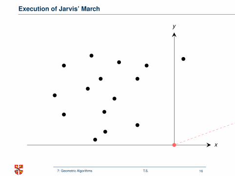
Execution of Jarvis’ March
x
y
x
y
x
y
x
y
x
y
x
y
x
y
7: Geometric Algorithms T.S. 16

Execution of Jarvis’ March
x
y
x
y
x
y
x
y
x
y
x
y
x
y
7: Geometric Algorithms T.S. 16

Execution of Jarvis’ March
x
y
x
y
x
y
x
y
x
y
x
y
x
y
7: Geometric Algorithms T.S. 16
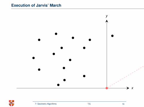
Execution of Jarvis’ March
x
y
x
y
x
y
x
y
x
y
x
y
x
y
7: Geometric Algorithms T.S. 16

Execution of Jarvis’ March
x
y
x
y
x
y
x
y
x
y
x
y
x
y
7: Geometric Algorithms T.S. 16

Execution of Jarvis’ March
x
y
x
y
x
y
x
y
x
y
x
y
x
y
7: Geometric Algorithms T.S. 16

Execution of Jarvis’ March
x
y
x
y
x
y
x
y
x
y
x
y
x
y
7: Geometric Algorithms T.S. 16

Execution of Jarvis’ March
x
y
x
y
x
y
x
y
x
y
x
y
x
y
7: Geometric Algorithms T.S. 16

Execution of Jarvis’ March
x
y
x
y
x
y
x
y
x
y
x
y
x
y
7: Geometric Algorithms T.S. 16

Execution of Jarvis’ March
x
y
x
y
x
y
x
y
x
y
x
y
x
y
7: Geometric Algorithms T.S. 16

Execution of Jarvis’ March
x
y
x
y
x
y
x
y
x
y
x
y
x
y
7: Geometric Algorithms T.S. 16

Execution of Jarvis’ March
x
y
x
y
x
y
x
y
x
y
x
y
x
y
7: Geometric Algorithms T.S. 16
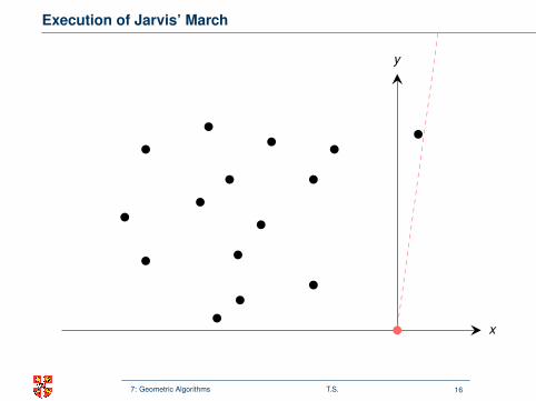
Execution of Jarvis’ March
x
y
x
y
x
y
x
y
x
y
x
y
x
y
7: Geometric Algorithms T.S. 16

Execution of Jarvis’ March
x
y
x
y
x
y
x
y
x
y
x
y
x
y
7: Geometric Algorithms T.S. 16
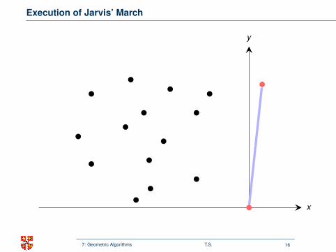
Execution of Jarvis’ March
x
y
x
y
x
y
x
y
x
y
x
y
x
y
7: Geometric Algorithms T.S. 16

Execution of Jarvis’ March
x
y
x
y
x
y
x
y
x
y
x
y
x
y
7: Geometric Algorithms T.S. 16

Execution of Jarvis’ March
x
y
x
y
x
y
x
y
x
y
x
y
x
y
7: Geometric Algorithms T.S. 16

Execution of Jarvis’ March
x
y
x
y
x
y
x
y
x
y
x
y
x
y
7: Geometric Algorithms T.S. 16

Execution of Jarvis’ March
x
y
x
y
x
y
x
y
x
y
x
y
x
y
7: Geometric Algorithms T.S. 16

Execution of Jarvis’ March
x
y
x
y
x
y
x
y
x
y
x
y
x
y
7: Geometric Algorithms T.S. 16

Execution of Jarvis’ March
x
y
x
y
x
y
x
y
x
y
x
y
x
y
7: Geometric Algorithms T.S. 16

Execution of Jarvis’ March
x
y
x
y
x
y
x
y
x
y
x
y
x
y
7: Geometric Algorithms T.S. 16
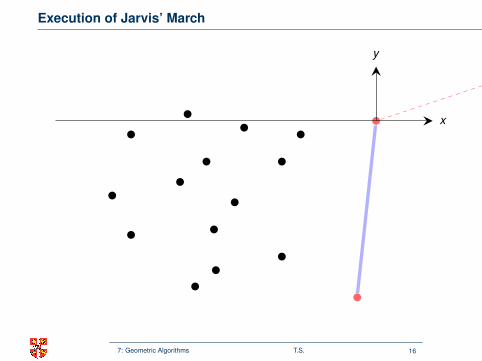
Execution of Jarvis’ March
x
y
x
y
x
y
x
y
x
y
x
y
x
y
7: Geometric Algorithms T.S. 16

Execution of Jarvis’ March
x
y
x
y
x
y
x
y
x
y
x
y
x
y
7: Geometric Algorithms T.S. 16

Execution of Jarvis’ March
x
y
x
y
x
y
x
y
x
y
x
y
x
y
7: Geometric Algorithms T.S. 16

Execution of Jarvis’ March
x
y
x
y
x
y
x
y
x
y
x
y
x
y
7: Geometric Algorithms T.S. 16

Execution of Jarvis’ March
x
y
x
y
x
y
x
y
x
y
x
y
x
y
7: Geometric Algorithms T.S. 16
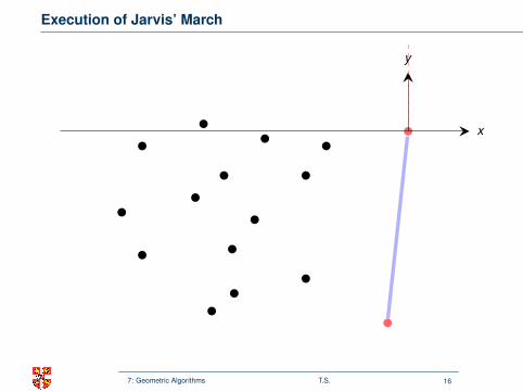
Execution of Jarvis’ March
x
y
x
y
x
y
x
y
x
y
x
y
x
y
7: Geometric Algorithms T.S. 16

Execution of Jarvis’ March
x
y
x
y
x
y
x
y
x
y
x
y
x
y
7: Geometric Algorithms T.S. 16

Execution of Jarvis’ March
x
y
x
y
x
y
x
y
x
y
x
y
x
y
7: Geometric Algorithms T.S. 16

Execution of Jarvis’ March
x
y
x
y
x
y
x
y
x
y
x
y
x
y
7: Geometric Algorithms T.S. 16

Execution of Jarvis’ March
x
y
x
y
x
y
x
y
x
y
x
y
x
y
7: Geometric Algorithms T.S. 16

Execution of Jarvis’ March
x
y
x
y
x
y
x
y
x
y
x
y
x
y
7: Geometric Algorithms T.S. 16
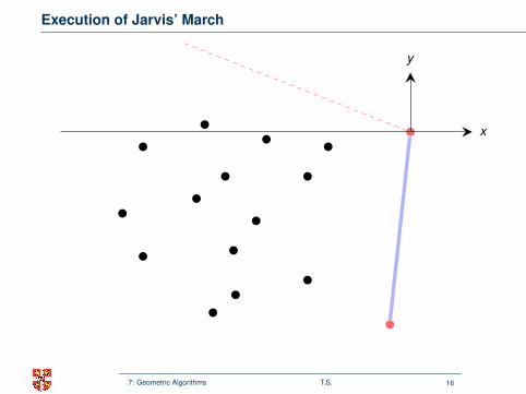
Execution of Jarvis’ March
x
y
x
y
x
y
x
y
x
y
x
y
x
y
7: Geometric Algorithms T.S. 16

Execution of Jarvis’ March
x
y
x
y
x
y
x
y
x
y
x
y
x
y
7: Geometric Algorithms T.S. 16

Execution of Jarvis’ March
x
y
x
y
x
y
x
y
x
y
x
y
x
y
7: Geometric Algorithms T.S. 16

Execution of Jarvis’ March
x
y
x
y
x
y
x
y
x
y
x
y
x
y
7: Geometric Algorithms T.S. 16
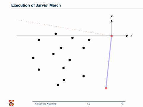
Execution of Jarvis’ March
x
y
x
y
x
y
x
y
x
y
x
y
x
y
7: Geometric Algorithms T.S. 16

Execution of Jarvis’ March
x
y
x
y
x
y
x
y
x
y
x
y
x
y
7: Geometric Algorithms T.S. 16

Execution of Jarvis’ March
x
y
x
y
x
y
x
y
x
y
x
y
x
y
7: Geometric Algorithms T.S. 16
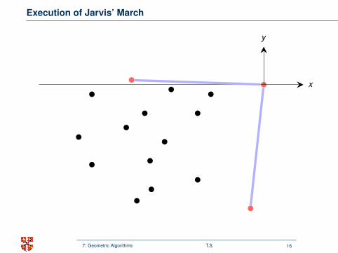
Execution of Jarvis’ March
x
y
x
y
x
y
x
y
x
y
x
y
x
y
7: Geometric Algorithms T.S. 16

Execution of Jarvis’ March
x
y
x
y
x
y
x
y
x
y
x
y
x
y
7: Geometric Algorithms T.S. 16

Execution of Jarvis’ March
x
y
x
y
x
y
x
y
x
y
x
y
x
y
7: Geometric Algorithms T.S. 16

Execution of Jarvis’ March
x
y
x
y
x
y
x
y
x
y
x
y
x
y
7: Geometric Algorithms T.S. 16
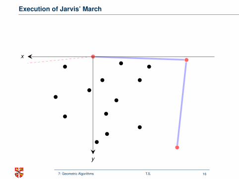
Execution of Jarvis’ March
x
y
x
y
x
y
x
y
x
y
x
y
x
y
7: Geometric Algorithms T.S. 16

Execution of Jarvis’ March
x
y
x
y
x
y
x
y
x
y
x
y
x
y
7: Geometric Algorithms T.S. 16

Execution of Jarvis’ March
x
y
x
y
x
y
x
y
x
y
x
y
x
y
7: Geometric Algorithms T.S. 16
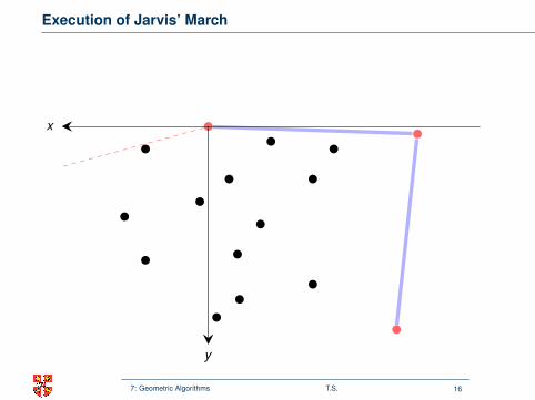
Execution of Jarvis’ March
x
y
x
y
x
y
x
y
x
y
x
y
x
y
7: Geometric Algorithms T.S. 16

Execution of Jarvis’ March
x
y
x
y
x
y
x
y
x
y
x
y
x
y
7: Geometric Algorithms T.S. 16
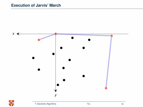
Execution of Jarvis’ March
x
y
x
y
x
y
x
y
x
y
x
y
x
y
7: Geometric Algorithms T.S. 16

Execution of Jarvis’ March
x
y
x
y
x
y
x
y
x
y
x
y
x
y
7: Geometric Algorithms T.S. 16

Execution of Jarvis’ March
x
y
x
y
x
y
x
y
x
y
x
y
x
y
7: Geometric Algorithms T.S. 16

Execution of Jarvis’ March
x
y
x
y
x
y
x
y
x
y
x
y
x
y
7: Geometric Algorithms T.S. 16

Execution of Jarvis’ March
x
y
x
y
x
y
x
y
x
y
x
y
x
y
7: Geometric Algorithms T.S. 16

Execution of Jarvis’ March
x
y
x
y
x
y
x
y
x
y
x
y
x
y
7: Geometric Algorithms T.S. 16

Execution of Jarvis’ March
x
y
x
y
x
y
x
y
x
y
x
y
x
y
7: Geometric Algorithms T.S. 16

Execution of Jarvis’ March
x
y
x
y
x
y
x
y
x
y
x
y
x
y
7: Geometric Algorithms T.S. 16

Execution of Jarvis’ March
x
y
x
y
x
y
x
y
x
y
x
y
x
y
7: Geometric Algorithms T.S. 16

Execution of Jarvis’ March
x
y
x
y
x
y
x
y
x
y
x
y
x
y
7: Geometric Algorithms T.S. 16
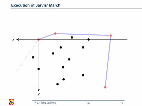
Execution of Jarvis’ March
x
y
x
y
x
y
x
y
x
y
x
y
x
y
7: Geometric Algorithms T.S. 16

Execution of Jarvis’ March
x
y
x
y
x
y
x
y
x
y
x
y
x
y
7: Geometric Algorithms T.S. 16

Execution of Jarvis’ March
x
y
x
y
x
y
x
y
x
y
x
y
x
y
7: Geometric Algorithms T.S. 16
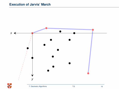
Execution of Jarvis’ March
x
y
x
y
x
y
x
y
x
y
x
y
x
y
7: Geometric Algorithms T.S. 16
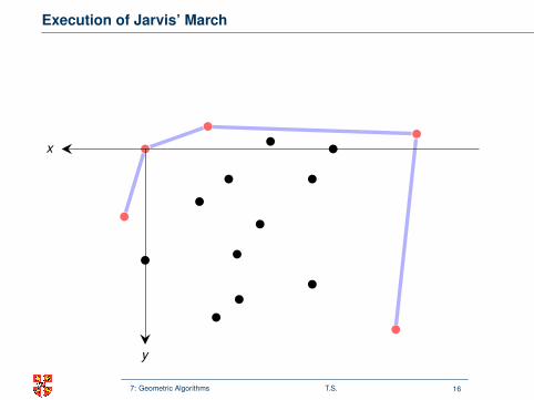
Execution of Jarvis’ March
x
y
x
y
x
y
x
y
x
y
x
y
x
y
7: Geometric Algorithms T.S. 16
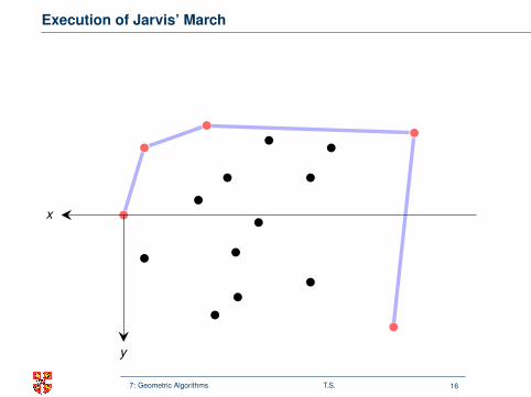
Execution of Jarvis’ March
x
y
x
y
x
y
x
y
x
y
x
y
x
y
7: Geometric Algorithms T.S. 16
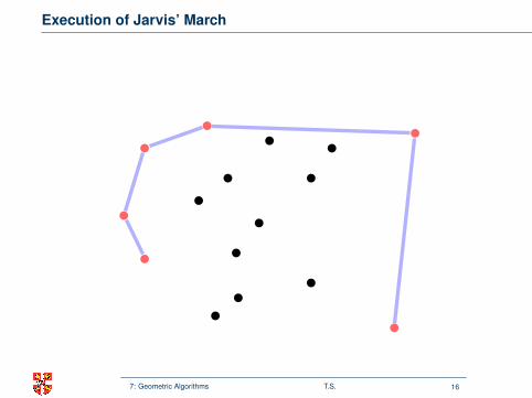
Execution of Jarvis’ March
x
y
x
y
x
y
x
y
x
y
x
y
x
y
7: Geometric Algorithms T.S. 16
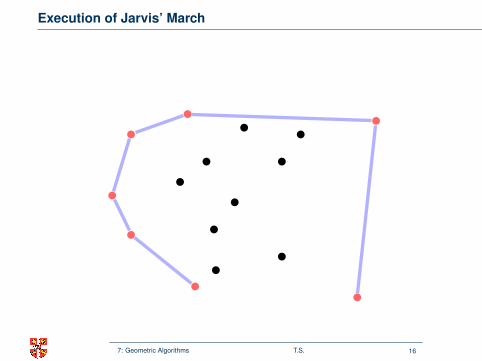
Execution of Jarvis’ March
x
y
x
y
x
y
x
y
x
y
x
y
x
y
7: Geometric Algorithms T.S. 16
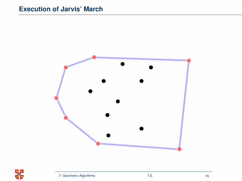
Execution of Jarvis’ March
x
y
x
y
x
y
x
y
x
y
x
y
x
y
7: Geometric Algorithms T.S. 16

Computing Convex Hull: Summary
natural backtracking algorithm
cross-product avoids computing polar angles
Runtime dominated by sorting O(n log n)
Graham’s Scan
proceeds like wrapping a gift
Runtime O(nh) output-sensitive
Jarvis’ March
Improves Graham’s scan only if h = O(log n)
There exists an algorithm with O(n log h) runtime!
cross product very powerful tool(avoids trigonometry and divison!)
take care of degenerate cases
Lessons Learned
7: Geometric Algorithms T.S. 17
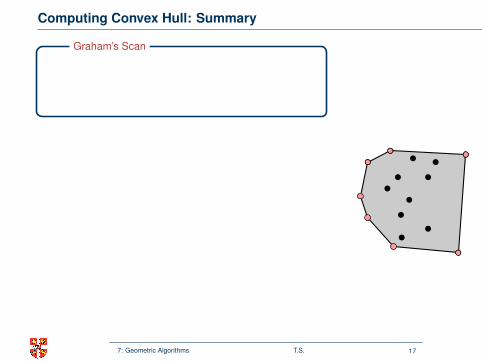
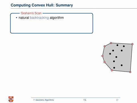
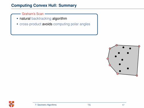
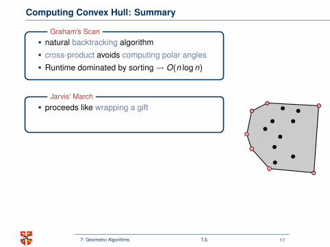
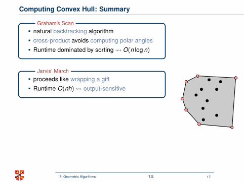
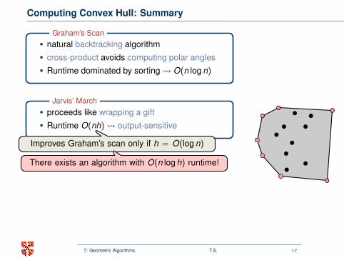
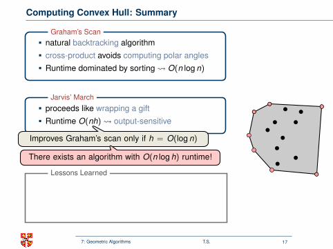
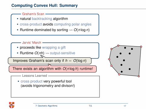
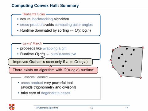
Outline
Introduction and Line Intersection
Convex Hull
Glimpse at (More) Advanced Algorithms
7: Geometric Algorithms T.S. 18
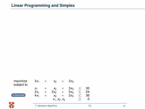
Linear Programming and Simplex
x1
x2
x3
(0, 0, 0)
(9, 0, 0)
(8.25, 0, 1.5)(8, 4, 0)
(0, 12, 0)
(0, 0, 4.8)
0
27
27.7528
12
9.6
maximize 3x1 + x2 + 2x3subject to
x1 + x2 + 3x3 ≤ 302x1 + 2x2 + 5x3 ≤ 244x1 + x2 + 2x3 ≤ 36
x1, x2, x3 ≥ 0Go to End
7: Geometric Algorithms T.S. 19
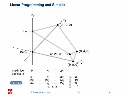
Linear Programming and Simplex
x1
x2
x3
(0, 0, 0)
(9, 0, 0)
(8.25, 0, 1.5)(8, 4, 0)
(0, 12, 0)
(0, 0, 4.8)
0
27
27.7528
12
9.6
maximize 3x1 + x2 + 2x3subject to
x1 + x2 + 3x3 ≤ 302x1 + 2x2 + 5x3 ≤ 244x1 + x2 + 2x3 ≤ 36
x1, x2, x3 ≥ 0Go to End
7: Geometric Algorithms T.S. 19
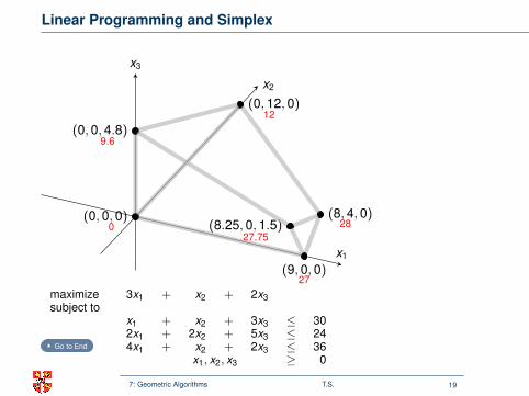
Linear Programming and Simplex
x1
x2
x3
(0, 0, 0)
(9, 0, 0)
(8.25, 0, 1.5)(8, 4, 0)
(0, 12, 0)
(0, 0, 4.8)
0
27
27.7528
12
9.6
maximize 3x1 + x2 + 2x3subject to
x1 + x2 + 3x3 ≤ 302x1 + 2x2 + 5x3 ≤ 244x1 + x2 + 2x3 ≤ 36
x1, x2, x3 ≥ 0Go to End
7: Geometric Algorithms T.S. 19

Linear Programming and Simplex
x1
x2
x3
(0, 0, 0)
(9, 0, 0)
(8.25, 0, 1.5)(8, 4, 0)
(0, 12, 0)
(0, 0, 4.8)
0
27
27.7528
12
9.6
maximize 3x1 + x2 + 2x3subject to
x1 + x2 + 3x3 ≤ 302x1 + 2x2 + 5x3 ≤ 244x1 + x2 + 2x3 ≤ 36
x1, x2, x3 ≥ 0Go to End
7: Geometric Algorithms T.S. 19
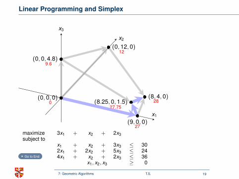
Linear Programming and Simplex
x1
x2
x3
(0, 0, 0)
(9, 0, 0)
(8.25, 0, 1.5)(8, 4, 0)
(0, 12, 0)
(0, 0, 4.8)
0
27
27.7528
12
9.6
maximize 3x1 + x2 + 2x3subject to
x1 + x2 + 3x3 ≤ 302x1 + 2x2 + 5x3 ≤ 244x1 + x2 + 2x3 ≤ 36
x1, x2, x3 ≥ 0Go to End
7: Geometric Algorithms T.S. 19
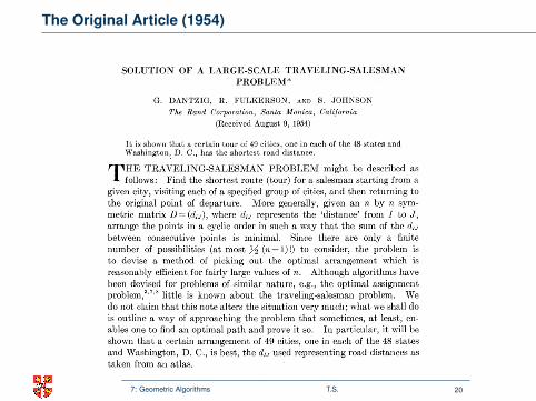
The Original Article (1954)
SOLUTION OF A LARGE-SCALE TRAVELING-SALESMAN PROBLEM*
G. DANTZIG, R. FULKERSON, AND S. JOHNSON The Rand Corporation, Santa Monica, California
(Received August 9, 1954)
It is shown that a certain tour of 49 cities, one in each of the 48 states and Washington, D. C., has the shortest road distance.
THE TRAVELING-SALESMAN PROBLEM might be described as follows: Find the shortest route (tour) for a salesman starting from a
given city, visiting each of a specified group of cities, and then returning to the original point of departure. More generally, given an n by n sym- metric matrix D= (d1i), where doi represents the 'distance' from I to J, arrange the points in a cyclic order in such a way that the sum of the d1j between consecutive points is minimal. Since there are only a finite number of possibilities (at most (n - 1)!) to consider, the problem is to devise a method of picking out the optimal arrangement which is reasonably efficient for fairly large values of n. Although algorithms have been devised for problems of similar nature, e.g., the optimal assignment problem,3"78 little is known about the traveling-salesman problem. We do not claim that this note alters the situation very much; what we shall do is outline a way of approaching the problem that sometimes, at least, en- ables one to find an optimal path and prove it so. In particular, it will be shown that a certain arrangement of 49 cities, one in each of the 48 states and Washington, D. C., is best, the djj used representing road distances as taken from an atlas.
* HISTORICAL NOTE: The origin of this problem is somewhat obscure. It appears to have been discussed informally among mathematicians at mathematics meetings for many years. Surprisingly little in the way of results has appeared in the mathematical literature.10 It may be that the minimal-distance tour problem was stimulated by the so-called Hamiltonian game' which is concerned with finding the number of different tours possible over a specified network. The latter problem is cited by some as the origin of group theory and has some connections with the famous Four-Color Conjecture.9 Merrill Flood (Columbia University) should be credited with stimulating interest in the traveling-salesman problem in many quar- ters. As early as 1937, he tried to obtain near optimal solutions in reference to routing of school buses. Both Flood and A. W. Tucker (Princeton University) re- call that they heard about the problem first in a seminar talk by Hassler Whitney at Princeton in 1934 (although Whitney, recently queried, does not seem to recall the problem). The relations between the traveling-salesman problem and the transportation problem of linear programming appear to have been first explored by M. Flood, J. Robinson, T. C. Koopmans, M. Beckmann, and later by I. Heller and H. Kuhn.4 5'6
393
7: Geometric Algorithms T.S. 20
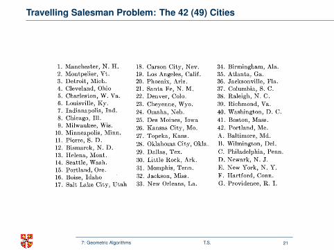
Travelling Salesman Problem: The 42 (49) Cities
394 DANTZIG, FULKERSON, AND JOHNSON
In order to try the method on a large problem, the following set of 49 cities, one in each state and the District of Columbia was selected:
1. Manchester, N. HI. 18. Carson City, Nev. 34. Birmingham, Ala. 2. Montpelier, Vt. 19. Los Angeles, Calif. 35. Atlanta, Ga. 3. Detroit, Mich. 20. Phoenix, Ariz. 36. Jacksonville, Fla. 4. Cleveland, Ohio 21. Santa Fe, N. M. 37. Columbia, S. C. 5. Charleston, W. Va. 22. Denver, Colo. 38. Raleigh, N. C. 6. Louisville, Ky. 23. Cheyenne, Wyo. 39. Richmond, Va. 7. Indianapolis, Ind. 24. Omaha, Neb. 40. Washington, D. C. 8. Chicago, Ill. 25. Des Moines, Iowa 41. Boston, Mass. 9. Milwaukee, Wis. 26. Kansas City, Mo. 42. Portland, Me.
10. Minneapolis, Minn. 27. Topeka, Kans. A. BaltimoreA Md.
12. Bismark, N. D. 28. Oklahoma City, Okla. B. Wilmington, Del. 13. Helenar, MNt. 29. Dallas, Tex. C. Philadelphia, Penn. 14. Seattle, Wash. 30. Little Rock, Ark. D. Newark, N. J. 15. Portland, Ore. 31. Memphis, Tenn. E. New York, N. Y. 16. Boise, Idaho 32. Jackson, Miss. F. Hartford, Conn. 17. Salt Lake City, Utah 33. New Orleans, La. G. Providence, R. I.
The reason for picking this particular set was that most of the road distances between them were easy to get from an atlas. The triangular table of distances between these cities (Table I) is part of the original one prepared by Bernice Brown of The Rand Corporation. It gives dj= K7 (di; - 11) (IJ = 1, 2, * , 42), where dii is the road distance in miles between I and J. The d1i have been rounded to the nearest integer. Certainly such a linear transformation does not alter the ordering of the tour lengths, although, of course, rounding could cause a tour that was not optimal in terms of the original mileage to become optimal in terms of the adjusted units used in this paper.
We will show that the tour (see Fig. 16) through the cities 1, 2, * *, 42 in this order is minimal for this subset of 42 cities. Moreover, since in driving from city 40 (Washington, D. C.) to city 41 (Boston, Massachusetts) by the shortest road distance one goes through A, B, * * *, G, successively, it follows that the tour through 49 cities 1, 2, .*, 40, A, B, *., G, 41, 42 in that order is also optimal.
PRELIMINARY NOTIONS
Whenever the road from I to J (in that order) is traveled, the value XIJ I is entered into the IJ element of a matrix; otherwise xiJ 0 is entered. A (directed) tour through n cities can now be thought of as a permutation matrix of order n which represents an n-cycle (we assume
* This particular transformation was chosen to make the d1j of the original table less than 256 which would permit compact storage of the distance table in binary representation; however, no use was made of this.
7: Geometric Algorithms T.S. 21
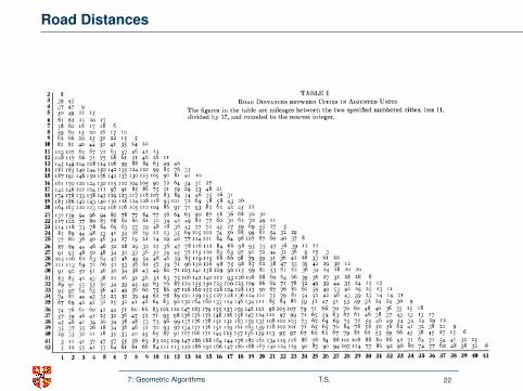
Road Distances
\0) cO
0O
00 n
00 e
cn C
- I- tr\
o C
NC
cl
cn cn -t 00
rN
C4
f 0
00\,O
0 tn
0 \ '
CC
, C
-) n
n\ ,O
c 0
t Q
>~~~~~~~~~~~~~~~~~~~~~~~~~~~~~~0
O.
0 q O
00 ol
o e
S~~~~~~~~~~~~~~~~~~~~~~~~~~~~~~~~i c
Ct'I t n
+ + t-oo
0 N
0
0 >
n cn
0 t-
z >
? ~~~~~~~~~~~~~~~~~~~~~~~~~~~~~C,
C,>
e ?-\,
roo +r" 0
e 0
? 0
? \o
0 c
o O
-
t" 00 ]00 C~
H
F ,,
E m
N
> +
> >
t +
+ ?
+?t +
O
4~~~~~~~~~~~~~~~~~~~~~~~~~~~~~~~~t
t Q
' m
+mO
>
tw#)b
.-w9
C-4 C
, C
4 Q
o \1-
\0 0
00 ac s
(0 iC
it
3 i0
t 00
I- ,
t1 ?
t (~~~~~~~n Itm
-< . r -\o
,O C
o ~O rO
o e 4
? 6>t I
00 M
M
f-
4 r > 00
C6 O
He %4
00) Q
o
an ~
b 6
on 6
H
X
? O
H
ct
+ tn
a> a> 4
0
S~~~~~~~~~~~~~~~~~~~~~~~~~~~~~~~~ cn r
Xbt
Xe\o \0
to 00
0 0 C
, O 0
On m
?i
? 00 0tC
I 0
0 0 00 .
00 ??o 00
L"O
tO
ci t es ) c i t'Thf?ci
.00' 000
cn st 0,
4i
~ ~4-~0) 00
ci C
) C
S) t~ 'tci\O
'-ci t0-~ ~, j.0
t 0- H
00
0C
i
cd -,o
o-o r-
coZ\~ 00
oo O
(7
0 ft+m
? s
SA?
c H
cn
ocall 0 0
0 W
C
S- o
tn o
cic~~-000000 00m
000-'-'M~
c 00c
Z t '.'
t0 t"-'t00
ci) 0
i 0
H
a -
tc t Z-000
ci 00
V-.
t O
0)' C
, 0
0 0
0"0o C
it N
', ''
kf ~~
)'t'ci0000 -~~~~~~~ci'C
00 0000
d I0~0
cic -p\
- 0
ci 0
0 O~~~~(~~f--~~
'-cic~~ 0',tci0',00 O
~~~~c-) ~~ t-0',tfl\,~~~~ ci00
0 C
X~~~~~~~~~~~~~~~~~~~~-
*0 C
' -
)+ mo v00
1c HF
tl C
A C
n C
,oo
t- o
_I
-o o
ci ~cif-~0
O
0 0
', -,
, 00
- t
r 0
o 0
C
C
c F4
i "
0 \O
'-ci00 ci
0N00\0
00 f--0000
-00X-=
~-A
tit- c
CA
"C
, 00
0N0c'c
ci 0
c c
i c00 roN
C
o\ r'
" 04
r r0
00 -\
"O
cm
C\
m
0 rb4
t- -t
r\. o
mO
O
CP\ 0
0 t3n C
n \ d
UN
CP\00 r-0
0 0
c 0
i 0
't '
0 N
,
' b0
""O
-- m
0 00
ci m
m00 0
't 'tci)00
080 ON
i00
fm cN
'
0 '0
'
0) ci
ci '-'~0
'-ci'~0 'tf--00 000000
ON
O
c \.O
ci
t- ',tr
~\C 0
wm
ci 'tci)'-ci00
00 f--i
c o
it N ci m
4 c
cO
n q- tn
W
0e ci'-
O~ci
0-?O ci
~i't"0 'ciO
NO
ci
c I-,0 O
N-
'-cic'o -,o
OC
) CO
C
)'c\ . tO
X
o0 0) Q
r0 F-
0 C
')'t t-4
4 0
0 f-
C=
f\ C
%
f 00
-*
c')t C
4 "
) 'cX
Io --\O
t -f
ON
0
ci c
c cn
t -
'tO-00
+
00 .)
- I
C, ) 0)
F- H
-00
0)0 O
N
ON
OC
= 0
-
\O
-CO
ciO
N rC
'
CA
o
't00 )o
n O
N O
rt
O
C' )\00
ci ' rcic
o 00- o"-
-
-0 00
000 '-
c ci
\i' C
) "0f--00
0 0
M
0 0
- O
N
CIA
O
0Ci-'
0 0
0- r0
00 C
0 ci C
00
0-ON
I- c
i '
- 0
-c c
0
ci i
- 00
0-0 c
0 'H
'tc C
n C
Y'o
-I '.
-0 00
Ot
) 0000
- C
A
11- -00
Ci ci
000 ?
W
0 C
c "
' -
- -
- O
- -00N
0
M'-
\o 0
c M
q0-~ 0N
cc-\,O
N'.0
"C ci
OO
N ci
\,O 00 \000
ci 't~~~ci00ciC
')C00c~~ic0
'-~ \O
Cic
CA
ic cn -,i,-4t
tj
t -
O
MO
O ',
O
O
V
- 0\,
C)
',) '.O
ON
NC
) 00
" C
) , --
-C
C'\00
0 ci
'I O
O
'4 .
Cl C
n 0 000
O
t 0
0M
- O
-???
r
f-o- 0
C,
-'t O
0 0
C0
' t --C
-) o
0 00
0\, - O
'ci00
OC
A
t 00
0 M
t
ci C
')'-ci f---
C''-
' t '3 t o ci o)0000
'-cit ' t't
0'-t c')'-+W
'c )
t ci
0 V
6 V
c
ci ci ~~~
~ 't'0 0-C
f- -'c
ci ('
''c )0
0'-- '-i-
-vi -l0'"
'CA
~ici c
0c 0 X
ci 0-
ci 0 't0"0
0-'-800c C"C
i 0
, 0
C')'t
', 00
C,)
cn i'c
tl '''
-i i'c
f cici
CA
ci I-
\- .-0
-N#-
CA
-,
c N
.t ''
C'.
iN-tc'c)
' o~~~~~~~~~~~~~~~~~~~~~~~C
H
7O
r- -1
r tn
3 \3 ,O
45
m
C4
CA
-n+<
t6> c n
'-f 0
O Ci4
\ - 'I-
i O
\cO
O
00
0)0 cn
')ci '-'-
i-I O
- O
N-C
f--"-,
'-) m
i ' 0
%,O
0O
'
tt-\ 00\ )O
c\
0 04
0) O
NC
f
ON
-\ C
> Y
C
f- O
ci'3 '
+ + +
)00 0 O
a -0
00 ooci
C",00
'-ci'-o C
-- ci
't'-ci f--f--
f-i '
i- 00
i cO
NcO
N
0 0-
0C
-
C'O
cim -c
-n --N
o 000
o 0 0w
'0000 1.
t-0 C
" ,'- r-
00 'T0
CO
N 00
O
sf-C-A
f-
' iti
c
Nm
m
M
) 'i s)
ooO
OO
y
QtN
130dt 000 C
~, O
i
Z o
o M
c \O
8-Q
-) C
\
S~~~~~~~diF~~~~~~~" r*tO
"_ G
e .-
Vd iU4("
N6~h
Neez
F#0 )
-mm
etm
mbo
mm
7: Geometric Algorithms T.S. 22
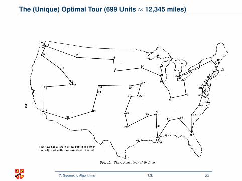
The (Unique) Optimal Tour (699 Units ≈ 12,345 miles)
C)
Ul)~~~~~
I X
4
0
CC
A
0~~~~~~~~~~0
* |
~~~A
./H
'-
fCs
E 4*
400 ~
~ ~
0
_~~~~~~~~~ V
40M
<
7: Geometric Algorithms T.S. 23
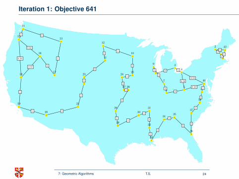
Iteration 1: Objective 641
1
12
2
3
3
4
4
5
5
6
6
7
7
8
8
9
9
10
10
11
11
12
1213
13
14
14
15
15
16
16
17
17
18
18
19
19
20
20
21
21
22
2223
2324
2425
25
26
2627
27
28
28
29
29
30
3031
31
32
32
33
33
34
3435
35
36
36
37
37
38
38
39
39
40
40
41
41
42
42
1
1
1
11
0.50
0.50
1
0.501
1
1
1
1
1
1
1
1
1
0.50
0.50
10.50
1
1 1
1
1
1
1
1
1
11
1
1
1
1
1
11
1
1
1
1
7: Geometric Algorithms T.S. 24
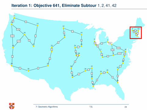
Iteration 1: Objective 641, Eliminate Subtour 1,2,41,42
1
12
2
3
3
4
4
5
5
6
6
7
7
8
8
9
9
10
10
11
11
12
1213
13
14
14
15
15
16
16
17
17
18
18
19
19
20
20
21
21
22
2223
2324
2425
25
26
2627
27
28
28
29
29
30
3031
31
32
32
33
33
34
3435
35
36
36
37
37
38
38
39
39
40
40
41
41
42
42
1
1
1
11
0.50
0.50
1
0.501
1
1
1
1
1
1
1
1
1
0.50
0.50
10.50
1
1 1
1
1
1
1
1
1
11
1
1
1
1
1
11
1
1
1
1
7: Geometric Algorithms T.S. 24

Iteration 2: Objective 676
1
12
2
3
3
4
4
5
5
6
6
7
7
8
8
9
9
10
10
11
11
12
1213
13
14
14
15
15
16
16
17
17
18
18
19
19
20
20
21
21
22
2223
2324
2425
25
26
2627
27
28
28
29
29
30
3031
31
32
32
33
33
34
3435
35
36
36
37
37
38
38
39
39
40
40
41
41
42
42
1 1
0.50
0.50
11
1
1
1
1
1
1
1
1
1
1
1
1
0.50
0.50
10.50
1
1 1
1
1
1
1
1
1
11
1
1
1
1
1
11
1
1
0.50
1
1
7: Geometric Algorithms T.S. 25
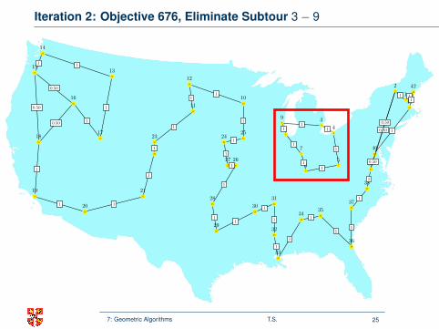
Iteration 2: Objective 676, Eliminate Subtour 3 − 9
1
12
2
3
3
4
4
5
5
6
6
7
7
8
8
9
9
10
10
11
11
12
1213
13
14
14
15
15
16
16
17
17
18
18
19
19
20
20
21
21
22
2223
2324
2425
25
26
2627
27
28
28
29
29
30
3031
31
32
32
33
33
34
3435
35
36
36
37
37
38
38
39
39
40
40
41
41
42
42
1 1
0.50
0.50
11
1
1
1
1
1
1
1
1
1
1
1
1
0.50
0.50
10.50
1
1 1
1
1
1
1
1
1
11
1
1
1
1
1
11
1
1
0.50
1
1
7: Geometric Algorithms T.S. 25

Iteration 3: Objective 681
1
12
2
3
3
4
4
5
5
6
6
7
7
8
8
9
9
10
10
11
11
12
1213
13
14
14
15
15
16
16
17
17
18
18
19
19
20
20
21
21
22
2223
2324
2425
25
26
2627
27
28
28
29
29
30
3031
31
32
32
33
33
34
3435
35
36
36
37
37
38
38
39
39
40
40
41
41
42
42
1 1
1
1
1
1
1
1
1
1
11
1
1
1
1
0.50
0.50
10.50
1
1 1
1
1
1
1 1
1
1
1
1
1
0.50
0.50
1
0.50
1
11
1
1
1
1
1
7: Geometric Algorithms T.S. 26
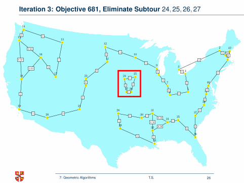
Iteration 3: Objective 681, Eliminate Subtour 24,25,26,27
1
12
2
3
3
4
4
5
5
6
6
7
7
8
8
9
9
10
10
11
11
12
1213
13
14
14
15
15
16
16
17
17
18
18
19
19
20
20
21
21
22
2223
2324
2425
25
26
2627
27
28
28
29
29
30
3031
31
32
32
33
33
34
3435
35
36
36
37
37
38
38
39
39
40
40
41
41
42
42
1 1
1
1
1
1
1
1
1
1
11
1
1
1
1
0.50
0.50
10.50
1
1 1
1
1
1
1 1
1
1
1
1
1
0.50
0.50
1
0.50
1
11
1
1
1
1
1
7: Geometric Algorithms T.S. 26

Iteration 4: Objective 682.5
1
12
2
3
3
4
4
5
5
6
6
7
7
8
8
9
9
10
10
11
11
12
1213
13
14
14
15
15
16
16
17
17
18
18
19
19
20
20
21
21
22
2223
2324
2425
25
26
2627
27
28
28
29
29
30
3031
31
32
32
33
33
34
3435
35
36
36
37
37
38
38
39
39
40
40
41
41
42
42
1 1
1
1
1
1
1
1
1
0.50
0.50
1
0.50
1
1
1
1
1
0.50
0.50
10.50
1
1 1
1
1
1
1
1
1
11
1
1
1
1
1
11
1
1
1
1
1
7: Geometric Algorithms T.S. 27
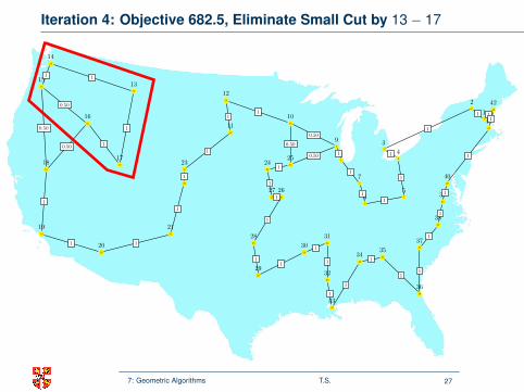
Iteration 4: Objective 682.5, Eliminate Small Cut by 13 − 17
1
12
2
3
3
4
4
5
5
6
6
7
7
8
8
9
9
10
10
11
11
12
1213
13
14
14
15
15
16
16
17
17
18
18
19
19
20
20
21
21
22
2223
2324
2425
25
26
2627
27
28
28
29
29
30
3031
31
32
32
33
33
34
3435
35
36
36
37
37
38
38
39
39
40
40
41
41
42
42
1 1
1
1
1
1
1
1
1
0.50
0.50
1
0.50
1
1
1
1
1
0.50
0.50
10.50
1
1 1
1
1
1
1
1
1
11
1
1
1
1
1
11
1
1
1
1
1
7: Geometric Algorithms T.S. 27
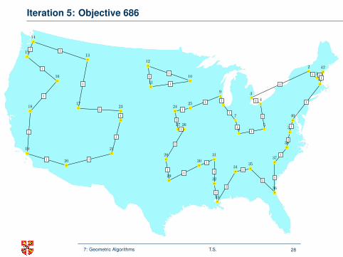
Iteration 5: Objective 686
1
12
2
3
3
4
4
5
5
6
6
7
7
8
8
9
9
10
10
11
11
12
1213
13
14
14
15
15
16
16
17
17
18
18
19
19
20
20
21
21
22
2223
2324
2425
25
26
2627
27
28
28
29
29
30
3031
31
32
32
33
33
34
3435
35
36
36
37
37
38
38
39
39
40
40
41
41
42
42
1 1
1
1
1
1
1
1
11
1
11
1
1
1
1
1
1
1
1 1
1
1
1
1
1
1
11
1
1
1
1
1
11
1
1
1
1
1
7: Geometric Algorithms T.S. 28
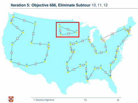
Iteration 5: Objective 686, Eliminate Subtour 10,11,12
1
12
2
3
3
4
4
5
5
6
6
7
7
8
8
9
9
10
10
11
11
12
1213
13
14
14
15
15
16
16
17
17
18
18
19
19
20
20
21
21
22
2223
2324
2425
25
26
2627
27
28
28
29
29
30
3031
31
32
32
33
33
34
3435
35
36
36
37
37
38
38
39
39
40
40
41
41
42
42
1 1
1
1
1
1
1
1
11
1
11
1
1
1
1
1
1
1
1 1
1
1
1
1
1
1
11
1
1
1
1
1
11
1
1
1
1
1
7: Geometric Algorithms T.S. 28

Iteration 6: Objective 686
1
12
2
3
3
4
4
5
5
6
6
7
7
8
8
9
9
10
10
11
11
12
1213
13
14
14
15
15
16
16
17
17
18
18
19
19
20
20
21
21
22
2223
2324
2425
25
26
2627
27
28
28
29
29
30
3031
31
32
32
33
33
34
3435
35
36
36
37
37
38
38
39
39
40
40
41
41
42
42
1 1
1
1
1
1
1
1
1
1
11
1
1
1
1
1
1
1
1
1 1
1
1
1
1
1
1
11
1
1
1
1
1
11
1
1
1
1
1
7: Geometric Algorithms T.S. 29
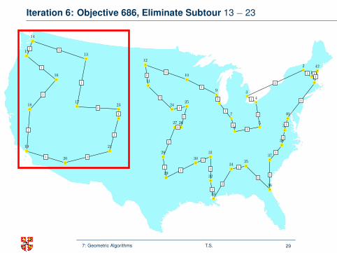
Iteration 6: Objective 686, Eliminate Subtour 13 − 23
1
12
2
3
3
4
4
5
5
6
6
7
7
8
8
9
9
10
10
11
11
12
1213
13
14
14
15
15
16
16
17
17
18
18
19
19
20
20
21
21
22
2223
2324
2425
25
26
2627
27
28
28
29
29
30
3031
31
32
32
33
33
34
3435
35
36
36
37
37
38
38
39
39
40
40
41
41
42
42
1 1
1
1
1
1
1
1
1
1
11
1
1
1
1
1
1
1
1
1 1
1
1
1
1
1
1
11
1
1
1
1
1
11
1
1
1
1
1
7: Geometric Algorithms T.S. 29
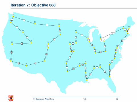
Iteration 7: Objective 688
1
12
2
3
3
4
4
5
5
6
6
7
7
8
8
9
9
10
10
11
11
12
1213
13
14
14
15
15
16
16
17
17
18
18
19
19
20
20
21
21
22
2223
2324
2425
25
26
2627
27
28
28
29
29
30
3031
31
32
32
33
33
34
3435
35
36
36
37
37
38
38
39
39
40
40
41
41
42
42
1 1
1
1
1
1
1
1
1
1
1
1
1
1
11
1
1
1
1
1 1
1
1
1
1
1
1
11
1
1
1
1
1
11
1
1
1
1
1
7: Geometric Algorithms T.S. 30
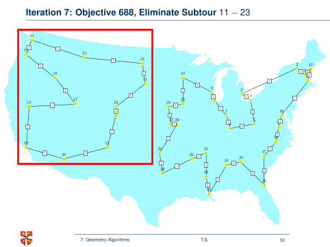
Iteration 7: Objective 688, Eliminate Subtour 11 − 23
1
12
2
3
3
4
4
5
5
6
6
7
7
8
8
9
9
10
10
11
11
12
1213
13
14
14
15
15
16
16
17
17
18
18
19
19
20
20
21
21
22
2223
2324
2425
25
26
2627
27
28
28
29
29
30
3031
31
32
32
33
33
34
3435
35
36
36
37
37
38
38
39
39
40
40
41
41
42
42
1 1
1
1
1
1
1
1
1
1
1
1
1
1
11
1
1
1
1
1 1
1
1
1
1
1
1
11
1
1
1
1
1
11
1
1
1
1
1
7: Geometric Algorithms T.S. 30

Iteration 8: Objective 697
1
12
2
3
3
4
4
5
5
6
6
7
7
8
8
9
9
10
10
11
11
12
1213
13
14
14
15
15
16
16
17
17
18
18
19
19
20
20
21
21
22
2223
2324
2425
25
26
2627
27
28
28
29
29
30
3031
31
32
32
33
33
34
3435
35
36
36
37
37
38
38
39
39
40
40
41
41
42
42
1 1
1
1
1
1
1
1
1
1
0.50
0.50
1
0.50 0.50
0.50
1
0.50
1
0.50
0.50
10.50
0.50
1
1 1
0.50
0.50
1
0.50
1
0.50 0.50
1
0.50
11
1
1
1
1
1
11
1
1
1
1
1
7: Geometric Algorithms T.S. 31
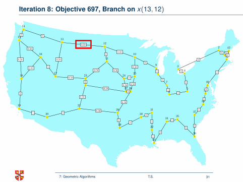
Iteration 8: Objective 697, Branch on x(13,12)
1
12
2
3
3
4
4
5
5
6
6
7
7
8
8
9
9
10
10
11
11
12
1213
13
14
14
15
15
16
16
17
17
18
18
19
19
20
20
21
21
22
2223
2324
2425
25
26
2627
27
28
28
29
29
30
3031
31
32
32
33
33
34
3435
35
36
36
37
37
38
38
39
39
40
40
41
41
42
42
1 1
1
1
1
1
1
1
1
1
0.50
0.50
1
0.50 0.50
0.50
1
0.50
1
0.50
0.50
10.50
0.50
1
1 1
0.50
0.50
1
0.50
1
0.50 0.50
1
0.50
11
1
1
1
1
1
11
1
1
1
1
1
7: Geometric Algorithms T.S. 31

Iteration 9, Branch a x(13,12) = 1: Objective 699 (Valid Tour)
1
12
2
3
3
4
4
5
5
6
6
7
7
8
8
9
9
10
10
11
11
12
1213
13
14
14
15
15
16
16
17
17
18
18
19
19
20
20
21
21
22
2223
2324
2425
25
26
2627
27
28
28
29
29
30
3031
31
32
32
33
33
34
3435
35
36
36
37
37
38
38
39
39
40
40
41
41
42
42
1 1
1
1
1
1
1
1
1
1
1
1
1
11
1
1
1
1
1 1
1
1
1 1
1
1
1
11
1
1
1
1
1
11
1
1
1
1
1
7: Geometric Algorithms T.S. 32

7: Geometric Algorithms T.S. 33

7: Geometric Algorithms T.S. 34
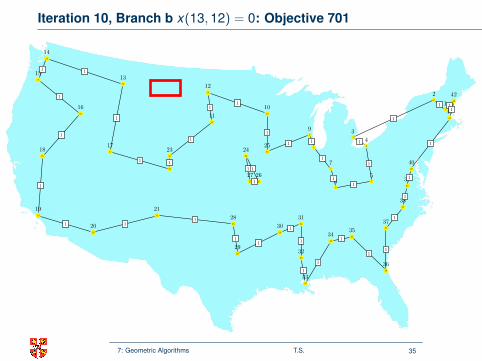
Iteration 10, Branch b x(13,12) = 0: Objective 701
1
12
2
3
3
4
4
5
5
6
6
7
7
8
8
9
9
10
10
11
11
12
1213
13
14
14
15
15
16
16
17
17
18
18
19
19
20
20
21
21
22
2223
2324
2425
25
26
2627
27
28
28
29
29
30
3031
31
32
32
33
33
34
3435
35
36
36
37
37
38
38
39
39
40
40
41
41
42
42
1 1
1
1
1
1
1
1
11
1
1
1
1
1
1
1
1
1
1
1
1 11
1
11
1
11
1
1
1
1
1
11
1
1
1
1
1
7: Geometric Algorithms T.S. 35

The End
Thank you for attending this course &Best wishes for the rest of your Tripos!
Don’t forget to visit the online feedback page!
Please send comments on the slides to:[email protected]
7: Geometric Algorithms T.S. 36


![Geometric Folding Algorithms - GitLabcba.mit.edu/events/13.03.scifab/Demaine.pdf · Geometric Folding Algorithms Linkages Paper ... Millibiology Project [MIT CBA] Millibiology Project](https://static.fdocuments.us/doc/165x107/5f098b217e708231d42754ea/geometric-folding-algorithms-geometric-folding-algorithms-linkages-paper-millibiology.jpg)


