Query by document via a decomposition-based two-level retrieval ...
Upload
nathan-erik-cobbCategory
view
287download
1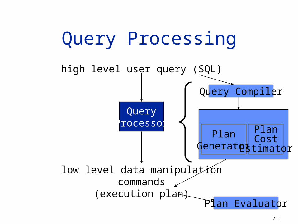
7-1
Query Processing
high level user query (SQL)
QueryProcessor
low level data manipulationcommands
(execution plan)
Query Compiler
PlanGenerator
PlanCost
Estimator
Plan Evaluator
7-2
Query Processing Components
Query language that is used SQL: “intergalactic dataspeak”
Query execution methodology The steps that one goes through in executing high-level
(declarative) user queries.
Query optimization How do we determine a good execution plan?
7-3
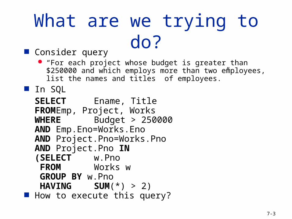
What are we trying to do? Consider query
“For each project whose budget is greater than $250000 and which employs more than two employees, list the names and titles of employees.”
In SQLSELECT Ename, TitleFROM Emp, Project, WorksWHERE Budget > 250000AND Emp.Eno=Works.Eno AND Project.Pno=Works.PnoAND Project.Pno IN
(SELECT w.Pno FROM Works w GROUP BY w.Pno HAVING SUM(*) > 2)
How to execute this query?
7-4
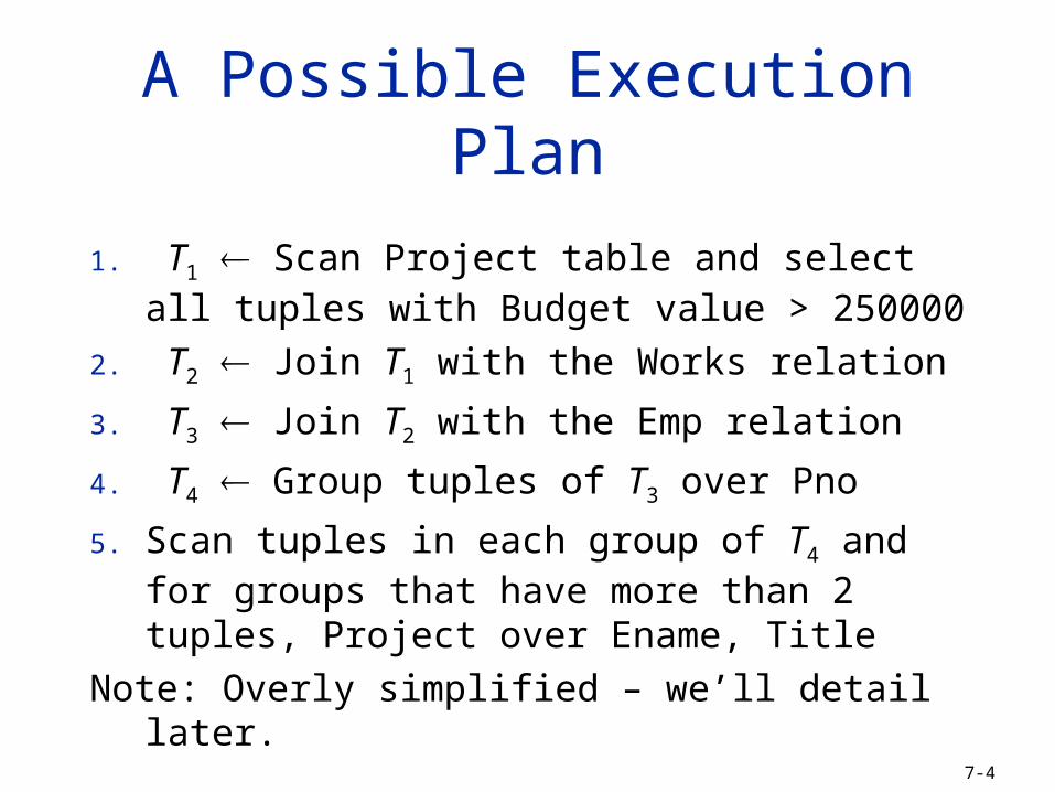
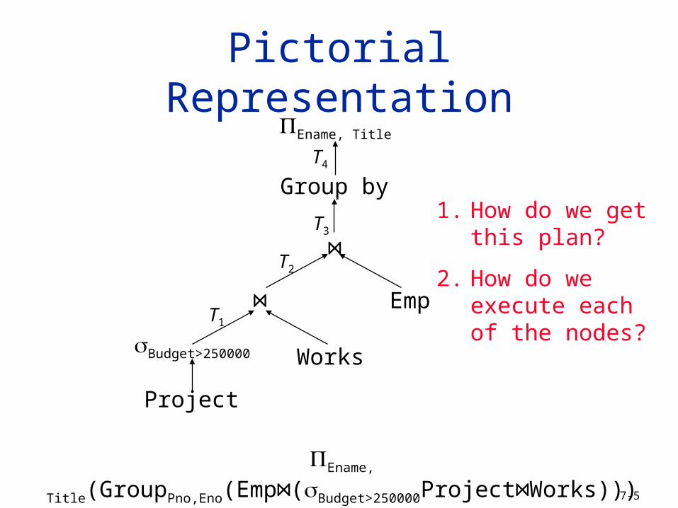
A Possible Execution Plan
1. T1 Scan Project table and select all tuples with Budget value > 250000
2. T2 Join T1 with the Works relation
3. T3 Join T2 with the Emp relation
4. T4 Group tuples of T3 over Pno
5. Scan tuples in each group of T4 and for groups that have more than 2 tuples, Project over Ename, Title
Note: Overly simplified – we’ll detail later.
7-5
Pictorial Representation
Project
Budget>250000 Works
⋈ Emp
⋈
Group by
Ename, Title
T1
T2
T3
T4
1. How do we get this plan?
2. How do we execute each of the nodes?
Ename, Title(GroupPno,Eno(Emp⋈(Budget>250000Project⋈Works)))
7-6
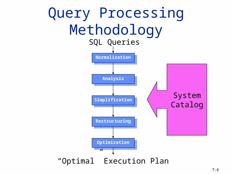
Query Processing Methodology
NormalizationNormalization
AnalysisAnalysis
SimplificationSimplification
RestructuringRestructuring
OptimizationOptimization
SQL Queries
“Optimal” Execution Plan
SystemCatalog
7-7
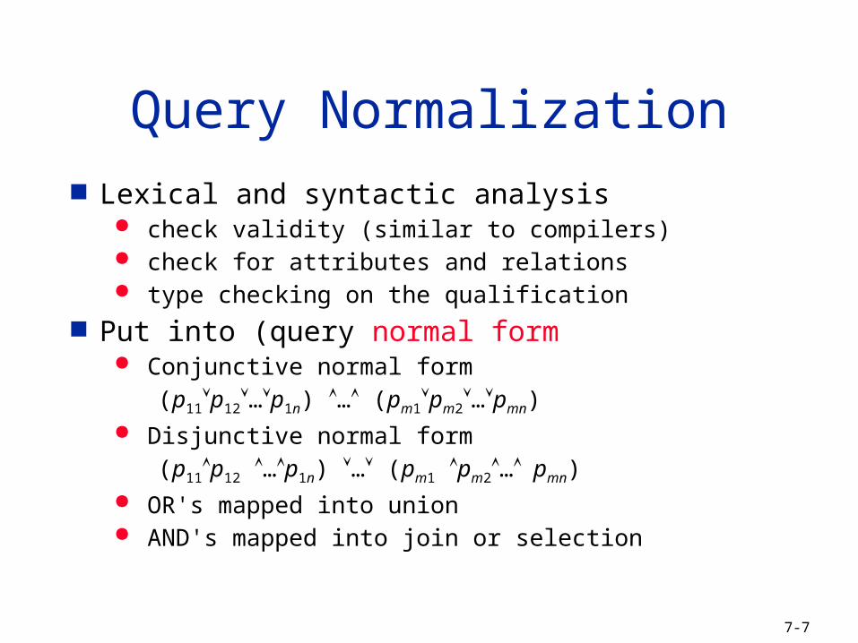
Lexical and syntactic analysis check validity (similar to compilers) check for attributes and relations type checking on the qualification
Put into (query normal form Conjunctive normal form
(p11p12…p1n) … (pm1pm2…pmn) Disjunctive normal form
(p11p12 …p1n) … (pm1 pm2…pmn) OR's mapped into union AND's mapped into join or selection
Query Normalization
7-8
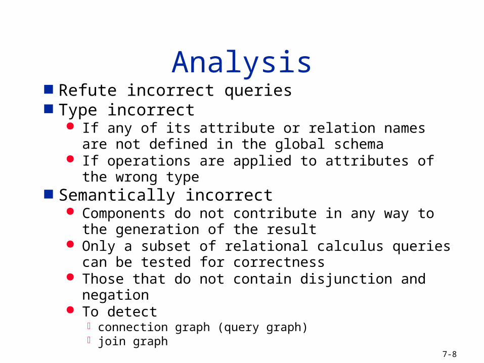
Refute incorrect queries Type incorrect
If any of its attribute or relation names are not defined in the global schema
If operations are applied to attributes of the wrong type Semantically incorrect
Components do not contribute in any way to the generation of the result
Only a subset of relational calculus queries can be tested for correctness
Those that do not contain disjunction and negation To detect
connection graph (query graph) join graph
Analysis
7-9
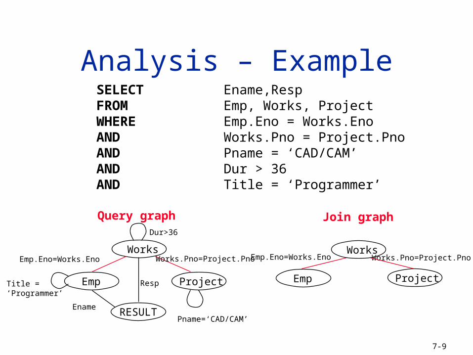
SELECT Ename,RespFROM Emp, Works, ProjectWHERE Emp.Eno = Works.Eno AND Works.Pno = Project.Pno AND Pname = ‘CAD/CAM’AND Dur > 36AND Title = ‘Programmer’
Query graph Join graph
Analysis – Example
Dur>36
Pname=‘CAD/CAM’
Ename
Emp.Eno=Works.Eno Works.Pno=Project.Pno
RESULT
Title =‘Programmer’
Resp
Works.Pno=Project.PnoEmp.Eno=Works.EnoWorks
ProjectEmp Emp Project
Works
7-10
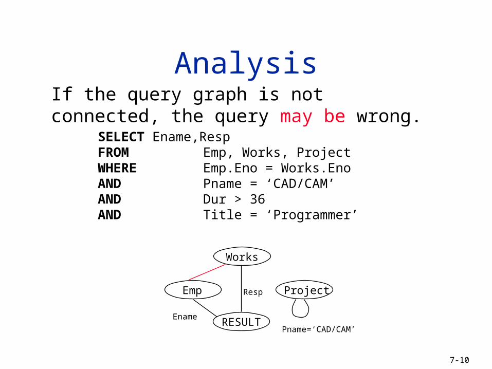
If the query graph is not connected, the query may be wrong.
SELECT Ename,RespFROM Emp, Works, ProjectWHERE Emp.Eno = Works.Eno AND Pname = ‘CAD/CAM’AND Dur > 36AND Title = ‘Programmer’
Analysis
Pname=‘CAD/CAM’
EnameRESULT
Resp
Works
ProjectEmp
7-11
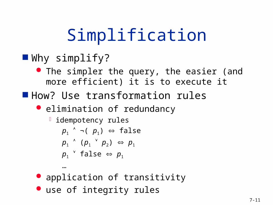
Why simplify? The simpler the query, the easier (and more efficient) it
is to execute it
How? Use transformation rules elimination of redundancy
idempotency rules
p1 ¬( p1) false
p1 (p1 p2) p1
p1 false p1
…
application of transitivity use of integrity rules
Simplification
7-12
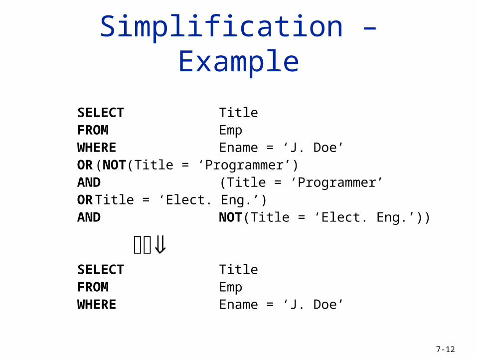
SELECT TitleFROM EmpWHERE Ename = ‘J. Doe’OR (NOT(Title = ‘Programmer’)AND (Title = ‘Programmer’ OR Title = ‘Elect. Eng.’) AND NOT(Title = ‘Elect. Eng.’))
SELECT Title FROM EmpWHERE Ename = ‘J. Doe’
Simplification – Example
7-13
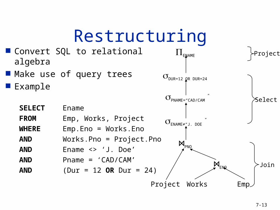
Convert SQL to relational algebra Make use of query trees Example
SELECT Ename
FROM Emp, Works, Project
WHERE Emp.Eno = Works.Eno
AND Works.Pno = Project.Pno
AND Ename <> ‘J. Doe’
AND Pname = ‘CAD/CAM’
AND (Dur = 12 OR Dur = 24)
RestructuringENAME
DUR=12 OR DUR=24
PNAME=“CAD/CAM”
ENAME≠“J. DOE”
Project Works Emp
Project
Select
Join
⋈PNO
⋈ENO
7-14
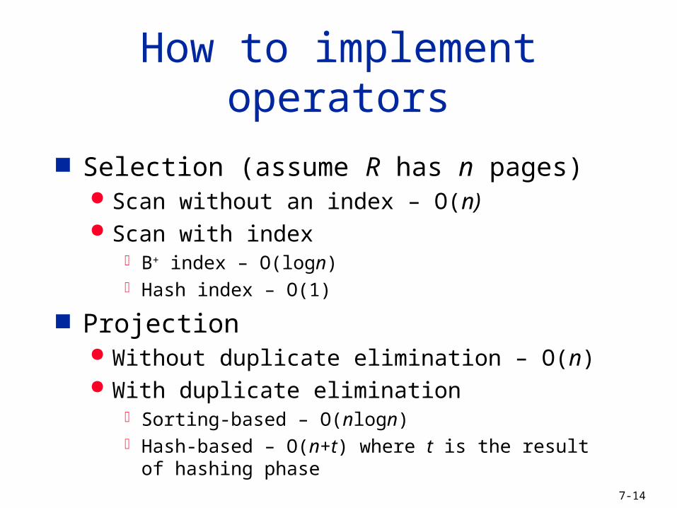
How to implement operators
Selection (assume R has n pages) Scan without an index – O(n) Scan with index
B+ index – O(logn) Hash index – O(1)
Projection Without duplicate elimination – O(n) With duplicate elimination
Sorting-based – O(nlogn) Hash-based – O(n+t) where t is the result of hashing phase
7-15
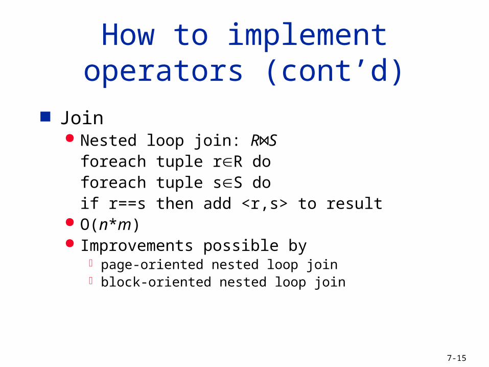
How to implement operators (cont’d)
Join Nested loop join: R⋈Sforeach tuple rR do
foreach tuple sS doif r==s then add <r,s> to
result O(n*m) Improvements possible by
page-oriented nested loop join block-oriented nested loop join
7-16
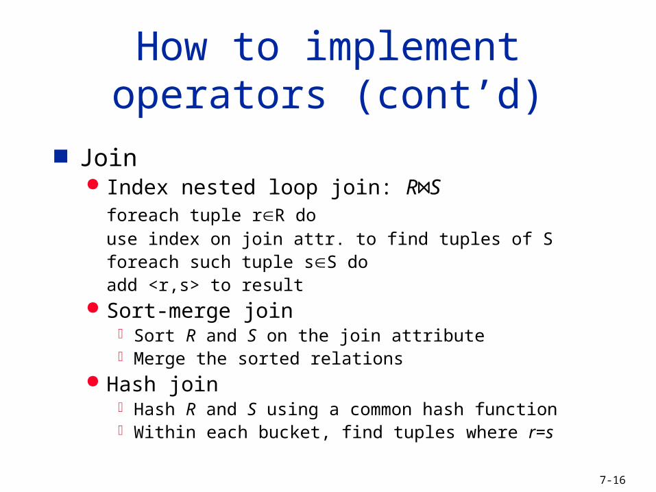
How to implement operators (cont’d)
Join Index nested loop join: R⋈Sforeach tuple rR do
use index on join attr. to find tuples of Sforeach such tuple sS do
add <r,s> to result Sort-merge join
Sort R and S on the join attribute Merge the sorted relations
Hash join Hash R and S using a common hash function Within each bucket, find tuples where r=s
7-17
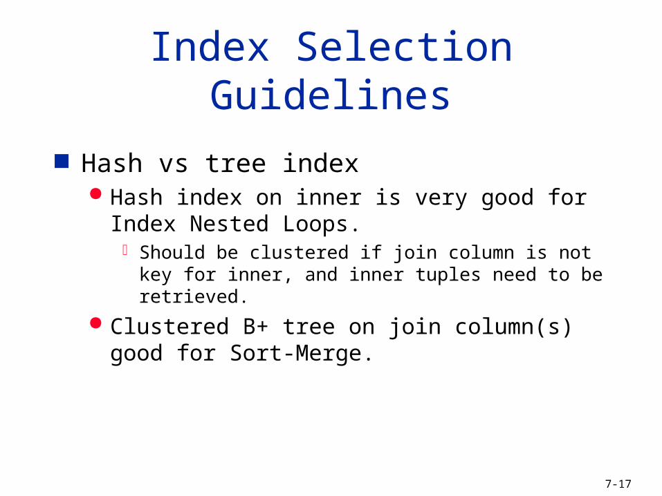
Index Selection Guidelines
Hash vs tree index Hash index on inner is very good for Index Nested
Loops. Should be clustered if join column is not key for inner, and
inner tuples need to be retrieved.
Clustered B+ tree on join column(s) good for Sort-Merge.
7-18
Example 1
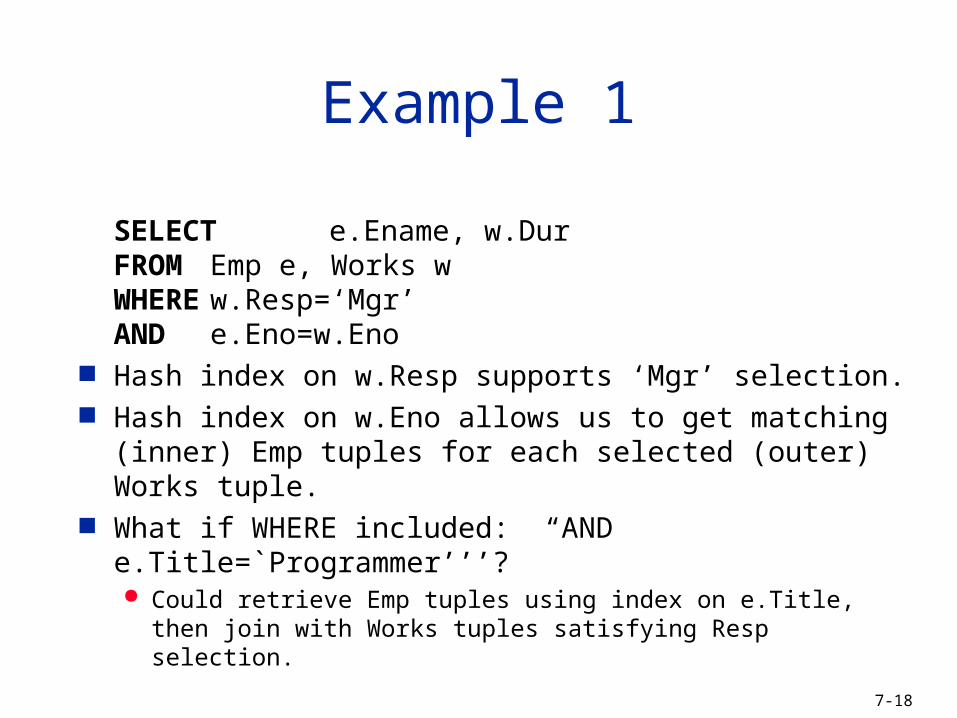
SELECT e.Ename, w.DurFROM Emp e, Works wWHERE w.Resp=‘Mgr’ AND e.Eno=w.Eno
Hash index on w.Resp supports ‘Mgr’ selection. Hash index on w.Eno allows us to get matching (inner) Emp
tuples for each selected (outer) Works tuple. What if WHERE included: “AND e.Title=`Programmer’’’?
Could retrieve Emp tuples using index on e.Title, then join with Works tuples satisfying Resp selection.
7-19
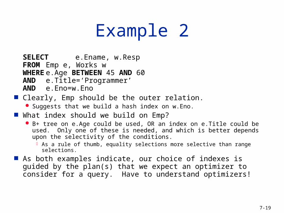
Example 2SELECT e.Ename, w.RespFROM Emp e, Works wWHERE e.Age BETWEEN 45 AND 60AND e.Title=‘Programmer’ AND e.Eno=w.Eno
Clearly, Emp should be the outer relation. Suggests that we build a hash index on w.Eno.
What index should we build on Emp? B+ tree on e.Age could be used, OR an index on e.Title could be used. Only one of
these is needed, and which is better depends upon the selectivity of the conditions. As a rule of thumb, equality selections more selective than range selections.
As both examples indicate, our choice of indexes is guided by the plan(s) that we expect an optimizer to consider for a query. Have to understand optimizers!
7-20
Examples of Clustering
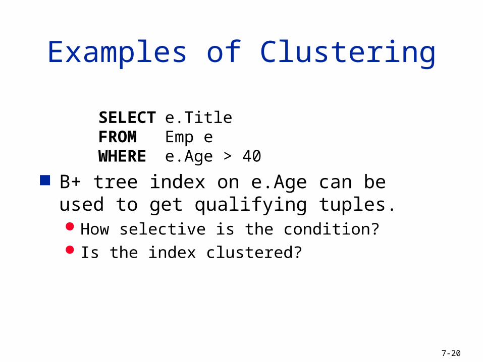
SELECT e.TitleFROM Emp eWHERE e.Age > 40
B+ tree index on e.Age can be used to get qualifying tuples. How selective is the condition? Is the index clustered?
7-21
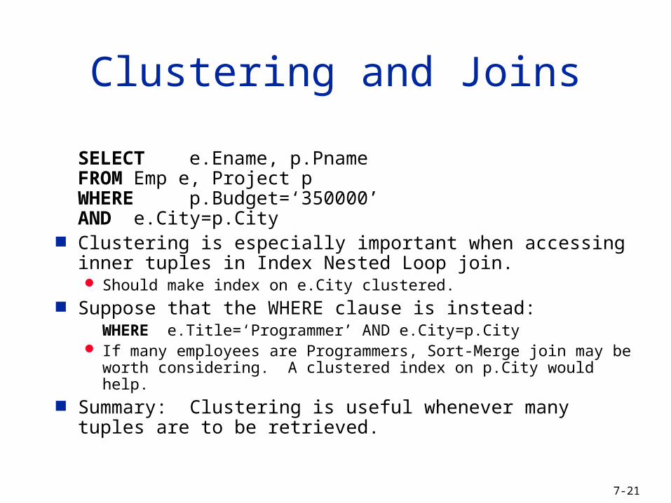
Clustering and Joins
SELECT e.Ename, p.PnameFROM Emp e, Project pWHERE p.Budget=‘350000’ AND e.City=p.City
Clustering is especially important when accessing inner tuples in Index Nested Loop join. Should make index on e.City clustered.
Suppose that the WHERE clause is instead:WHERE e.Title=‘Programmer’ AND e.City=p.City
If many employees are Programmers, Sort-Merge join may be worth considering. A clustered index on p.City would help.
Summary: Clustering is useful whenever many tuples are to be retrieved.
7-22
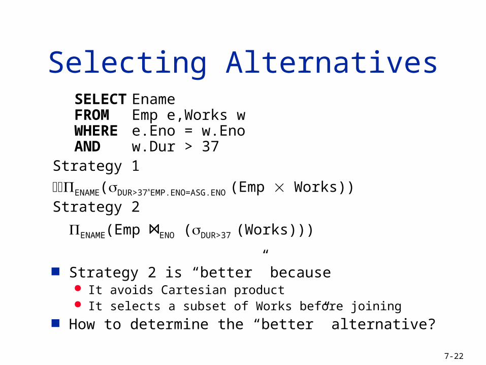
SELECT EnameFROM Emp e,Works wWHERE e.Eno = w.Eno AND w.Dur > 37
Strategy 1
ENAME(DUR>37EMP.ENO=ASG.ENO(Emp Works))Strategy 2
ENAME(Emp ⋈ENO (DUR>37 (Works)))
Strategy 2 is “better” because It avoids Cartesian product It selects a subset of Works before joining
How to determine the “better” alternative?
Selecting Alternatives
7-23
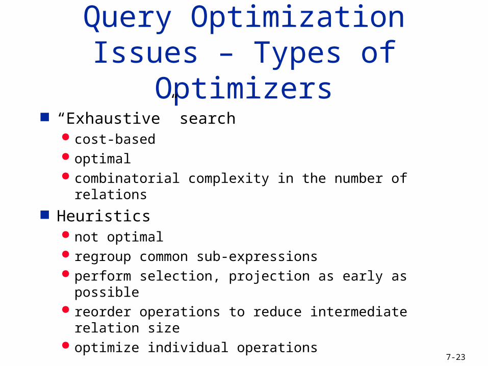
Query Optimization Issues – Types of Optimizers
“Exhaustive” search cost-based optimal combinatorial complexity in the number of relations
Heuristics not optimal regroup common sub-expressions perform selection, projection as early as possible reorder operations to reduce intermediate relation size optimize individual operations
7-24
Query Optimization Issues – Optimization Granularity
Single query at a time cannot use common intermediate results
Multiple queries at a time efficient if many similar queries decision space is much larger
7-25
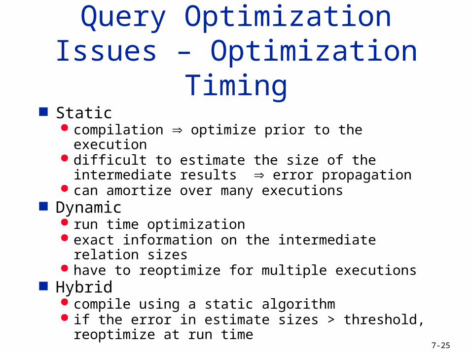
Query Optimization Issues – Optimization Timing
Static compilation optimize prior to the execution difficult to estimate the size of the intermediate results
error propagation can amortize over many executions
Dynamic run time optimization exact information on the intermediate relation sizes have to reoptimize for multiple executions
Hybrid compile using a static algorithm if the error in estimate sizes > threshold, reoptimize at
run time
7-26
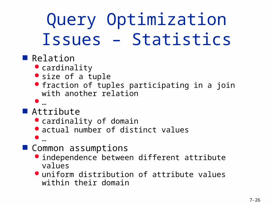
Query Optimization Issues – Statistics
Relation cardinality size of a tuple fraction of tuples participating in a join with another
relation …
Attribute cardinality of domain actual number of distinct values …
Common assumptions independence between different attribute values uniform distribution of attribute values within their domain
7-27
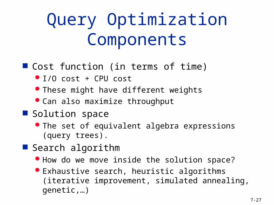
Query Optimization Components
Cost function (in terms of time) I/O cost + CPU cost These might have different weights Can also maximize throughput
Solution space The set of equivalent algebra expressions (query trees).
Search algorithm How do we move inside the solution space? Exhaustive search, heuristic algorithms (iterative
improvement, simulated annealing, genetic,…)
7-28
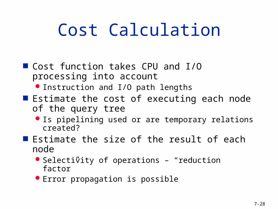
Cost Calculation
Cost function takes CPU and I/O processing into account Instruction and I/O path lengths
Estimate the cost of executing each node of the query tree Is pipelining used or are temporary relations created?
Estimate the size of the result of each node Selectivity of operations – “reduction factor” Error propagation is possible
7-29
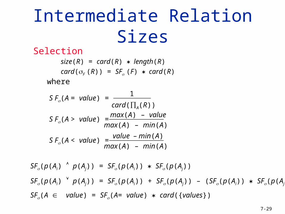
Selectionsize(R) = card(R) length(R)
card(F (R)) = SF (F) card(R)
where
Intermediate Relation Sizes
S F(A = value) = card(∏A(R))
1
S F(A > value) = max(A) – min(A) max(A) – value
S F(A < value) = max(A) – min(A) value – min(A)
SF(p(Ai) p(Aj)) = SF(p(Ai)) SF(p(Aj))
SF(p(Ai) p(Aj)) = SF(p(Ai)) + SF(p(Aj)) – (SF(p(Ai)) SF(p(Aj)))
SF(A value) = SF(A= value) card({values})
7-30
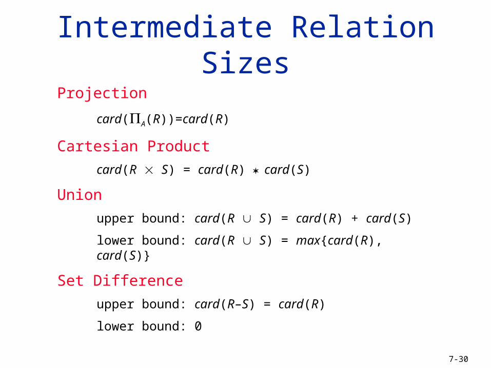
Projection
card(A(R))=card(R)
Cartesian Product
card(R S) = card(R) card(S)
Union
upper bound: card(R S) = card(R) + card(S)
lower bound: card(R S) = max{card(R), card(S)}
Set Difference
upper bound: card(R–S) = card(R)
lower bound: 0
Intermediate Relation Sizes
7-31
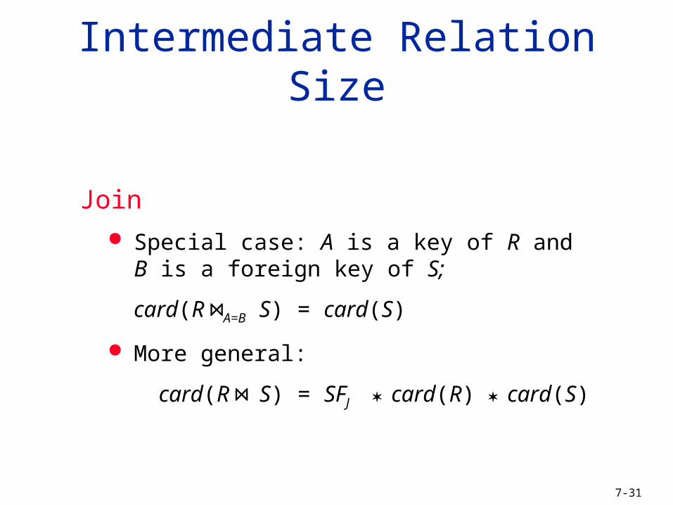
Join
Special case: A is a key of R and B is a foreign key of S;
card(R ⋈A=B S) = card(S)
More general:
card(R ⋈ S) = SFJ card(R) card(S)
Intermediate Relation Size
7-32
Search Space
Characterized by “equivalent” query plans Equivalence is defined in terms of equivalent query
results
Equivalent plans are generated by means of algebraic transformation rules
The cost of each plan may be different Focus on joins
7-33
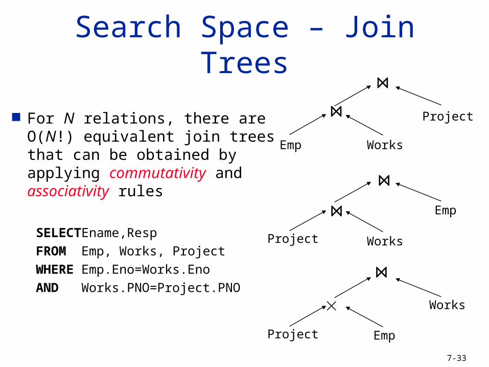
Search Space – Join Trees
For N relations, there are O(N!) equivalent join trees that can be obtained by applying commutativity and associativity rules
SELECT Ename,Resp
FROM Emp, Works, Project
WHERE Emp.Eno=Works.Eno
AND Works.PNO=Project.PNO
Project
WorksEmp
Project Works
Emp
Project
Works
Emp
⋈
⋈
⋈
⋈
⋈
7-34
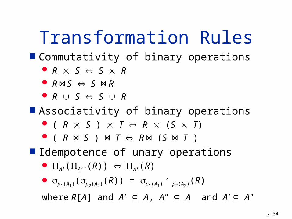
Commutativity of binary operations R S S R R ⋈ S S ⋈ R R S S R
Associativity of binary operations ( R S ) T R (S T) ( R ⋈ S ) ⋈ T R ⋈ (S ⋈ T )
Idempotence of unary operations A’(A’’(R)) A’(R)
p1(A1)(p2(A2)(R)) = p1(A1) p2(A2)(R)
where R[A] and A' A, A" A and A' A"
Transformation Rules
7-35
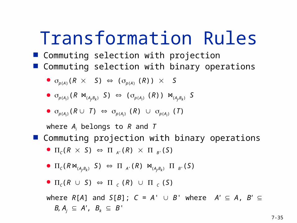
Commuting selection with projection Commuting selection with binary operations
p(A)(R S) (p(A) (R)) S
p(Ai)(R ⋈(Aj,Bk) S) (p(Ai)
(R)) ⋈(Aj,Bk) S
p(Ai)(R T) p(Ai)
(R) p(Ai) (T)
where Ai belongs to R and T
Commuting projection with binary operations C(R S) A’(R) B’(S)
C(R ⋈(Aj,Bk) S) A’(R) ⋈(Aj,Bk) B’(S)
C(R S) C (R) C (S)
where R[A] and S[B]; C = A' B' where A' A, B' B, Aj A', Bk B'
Transformation Rules
7-36
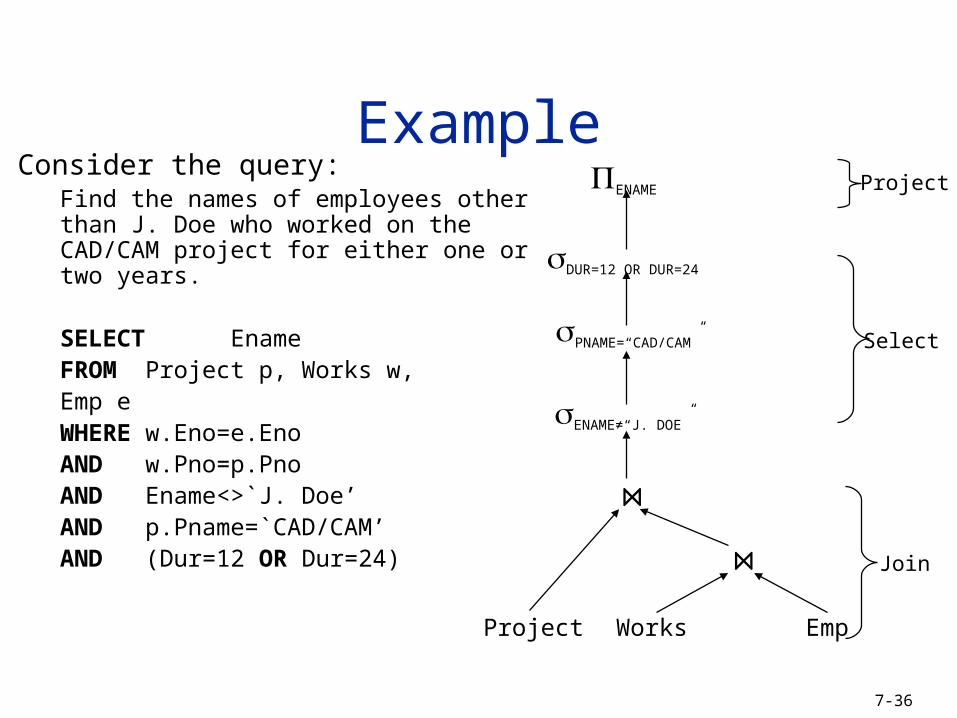
ExampleConsider the query:
Find the names of employees other than J. Doe who worked on the CAD/CAM project for either one or two years.
SELECT EnameFROM Project p, Works w,
Emp eWHERE w.Eno=e.EnoAND w.Pno=p.PnoAND Ename<>`J. Doe’AND p.Pname=`CAD/CAM’AND (Dur=12 OR Dur=24)
ENAME
DUR=12 OR DUR=24
PNAME=“CAD/CAM”
ENAME≠“J. DOE”
Project Works Emp
Project
Select
Join
⋈
⋈
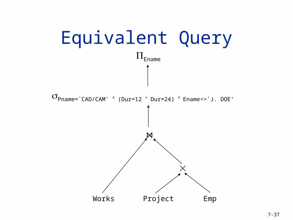
7-37
Equivalent QueryEname
Pname=`CAD/CAM’ (Dur=12 Dur=24) Ename<>`J. DOE’
ProjectWorks Emp
⋈
7-38
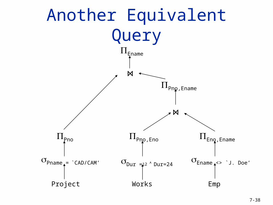
Emp
Ename
Ename <> `J. Doe’
WorksProject
Eno,Ename
Pname = `CAD/CAM’
Pno
Dur =12 Dur=24
Pno,Eno
Pno,Ename
Another Equivalent Query
⋈
⋈
7-39
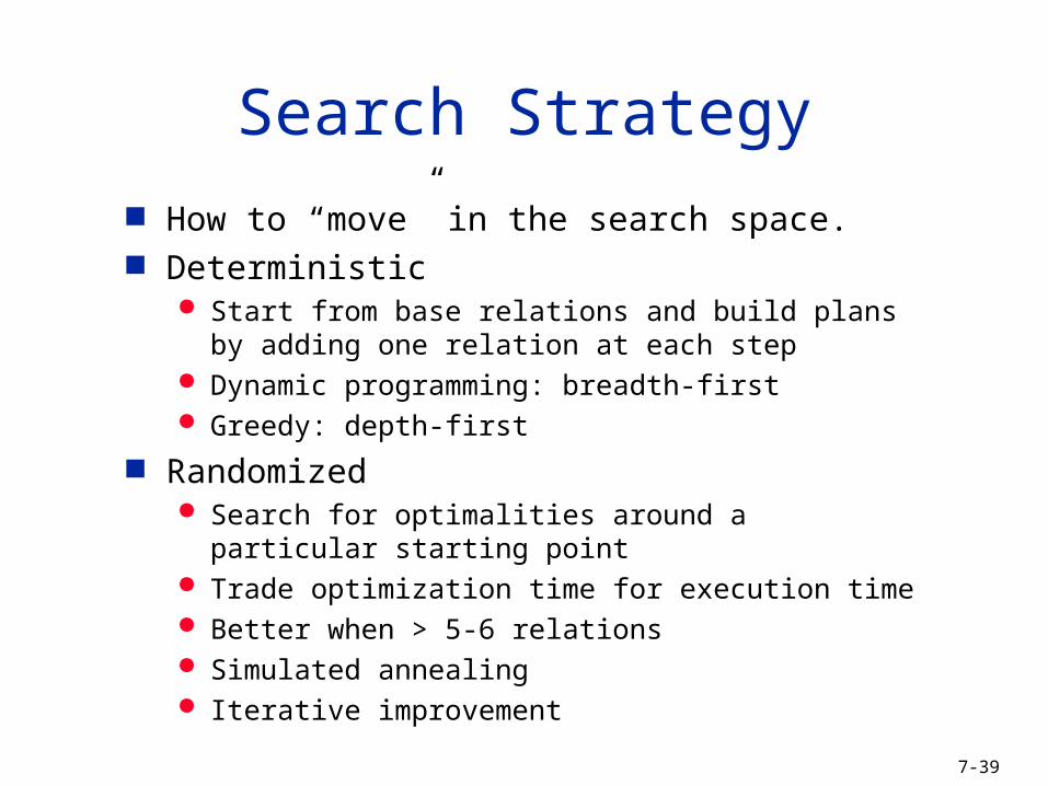
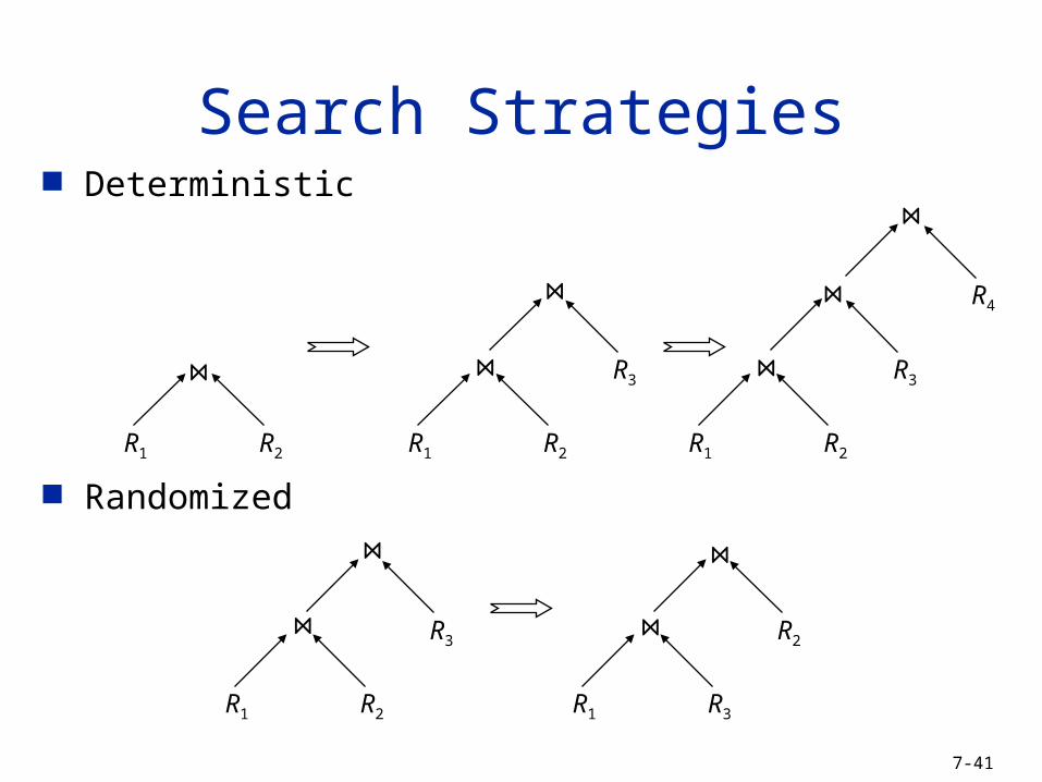
Search Strategy
How to “move” in the search space. Deterministic
Start from base relations and build plans by adding one relation at each step
Dynamic programming: breadth-first Greedy: depth-first
Randomized Search for optimalities around a particular starting point Trade optimization time for execution time Better when > 5-6 relations Simulated annealing Iterative improvement
7-40
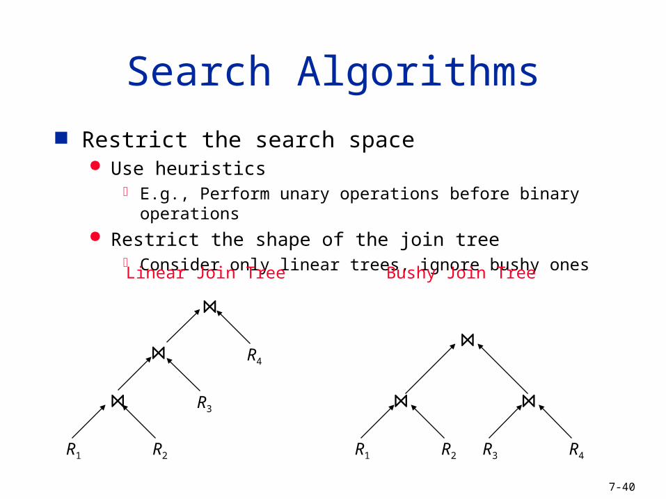
Search Algorithms
Restrict the search space Use heuristics
E.g., Perform unary operations before binary operations Restrict the shape of the join tree
Consider only linear trees, ignore bushy ones
R2R1
R3
R4
Linear Join Tree
R2R1 R4R3
Bushy Join Tree
⋈
⋈
⋈
⋈
⋈ ⋈
7-41
Search Strategies Deterministic
Randomized
R2R1
R3
R4
R2R1 R2R1
R3
R2R1
R3
R3R1
R2
⋈ ⋈
⋈
⋈
⋈
⋈
⋈
⋈
⋈
⋈
7-42
Summary Declarative SQL queries need to be converted into
low level execution plans These plans need to be optimized to find the
“best” plan Optimization involves
Search space: identifies the alternative plans and alternative execution algorithms for algebra operators
This is done by means of transformation rules Cost function: calculates the cost of executing each
plan CPU and I/O costs
Search algorithm: controls which alternative plans are investigated