Chapter 3 Atmospheric Thermodynamics, Instabilities, and ...

68 Atmospheric Thermodynamics
vertical force that acts on the slab of air between zand z � z due to the pressure of the surroundingair. Let the change in pressure in going from height zto height z � z be p, as indicated in Fig. 3.1.Because we know that pressure decreases withheight, p must be a negative quantity, and theupward pressure on the lower face of the shadedblock must be slightly greater than the downwardpressure on the upper face of the block. Therefore,the net vertical force on the block due to the verticalgradient of pressure is upward and given by the posi-tive quantity �p, as indicated in Fig. 3.1. For anatmosphere in hydrostatic balance, the balance offorces in the vertical requires that
or, in the limit as ,
(3.17)�p�z
� ���
z : 0
�p � ��z
Equation (3.17) is the hydrostatic equation.14 Itshould be noted that the negative sign in (3.17)ensures that the pressure decreases with increasingheight. Because � � 1�� (3.17) can be rearranged togive
(3.18)
If the pressure at height z is p(z), we have, from(3.17), above a fixed point on the Earth
or, because p(�) � 0,
(3.19)
That is, the pressure at height z is equal to the weightof the air in the vertical column of unit cross-sectional area lying above that level. If the mass ofthe Earth’s atmosphere were distributed uniformlyover the globe, retaining the Earth’s topographyin its present form, the pressure at sea level wouldbe 1.013 � 105 Pa, or 1013 hPa, which is referred toas 1 atmosphere (or 1 atm).
3.2.1 Geopotential
The geopotential at any point in the Earth’satmosphere is defined as the work that must bedone against the Earth’s gravitational field to raisea mass of 1 kg from sea level to that point. In otherwords, is the gravitational potential per unitmass. The units of geopotential are J kg�1 or m2 s�2.The force (in newtons) acting on 1 kg at height zabove sea level is numerically equal to �. The work(in joules) in raising 1 kg from z to z � dz is �dz;therefore
or, using (3.18),
(3.20)d � �dz � ��dp
d � �dz
p(z) � ��
z��dz
��p (�)
p (z)
dp � ��
z��dz
�dz � ��dp
Column with unit cross-sectional area
Pressure = p + δp
Pressure = p
Ground
z
–δp
gρδz
δz
Fig. 3.1 Balance of vertical forces in an atmosphere inwhich there are no vertical accelerations (i.e., an atmospherein hydrostatic balance). Small blue arrows indicate the down-ward force exerted on the air in the shaded slab due to thepressure of the air above the slab; longer blue arrows indicatethe upward force exerted on the shaded slab due to the pres-sure of the air below the slab. Because the slab has a unitcross-sectional area, these two pressures have the samenumerical values as forces. The net upward force due to thesepressures (�p) is indicated by the upward-pointing thickblack arrow. Because the incremental pressure change p is anegative quantity, �p is positive. The downward-pointingthick black arrow is the force acting on the shaded slab dueto the mass of the air in this slab.
14 In accordance with Eq. (1.3), the left-hand side of (3.17) is written in partial differential notation, i.e., �p��z, because the variation ofpressure with height is taken with other independent variables held constant.
P732951-Ch03.qxd 9/12/05 7:41 PM Page 68

70 Atmospheric Thermodynamics
Above the turbopause the vertical distribution ofgases is largely controlled by molecular diffusion anda scale height may then be defined for each of theindividual gases in air. Because for each gas the scaleheight is proportional to the gas constant for a unitmass of the gas, which varies inversely as the molecu-lar weight of the gas [see, for example (3.13)], thepressures (and densities) of heavier gases fall offmore rapidly with height above the turbopause thanthose of lighter gases.
Exercise 3.2 If the ratio of the number density ofoxygen atoms to the number density of hydrogenatoms at a geopotential height of 200 km above theEarth’s surface is 105, calculate the ratio of the num-ber densities of these two constituents at a geopoten-tial height of 1400 km. Assume an isothermalatmosphere between 200 and 1400 km with a tem-perature of 2000 K.
Solution: At these altitudes, the distribution ofthe individual gases is determined by diffusion andtherefore by (3.26). Also, at constant temperature,the ratio of the number densities of two gases isequal to the ratio of their pressures. From (3.26)
From the definition of scale height (3.27) and analo-gous expressions to (3.11) for oxygen and hydrogenatoms and the fact that the atomic weights of oxygenand hydrogen are 16 and 1, respectively, we have at2000 K
and
� 1.695 � 106 m
Hhyd �1000R*
1 20009.81
m � 8.3145 2 � 106
9.81 m
� 0.106 � 106 m
Hoxy �1000R*
16 20009.81
m �8.3145
16 2 � 106
9.81 m
� 105 exp ��1200 km 1Hoxy
�1
Hhyd�
�(p200 km)oxy exp[�1200 km�Hoxy (km)](p200 km)hyd exp[�1200 km�Hhyd (km)]
(p1400 km)oxy
(p1400 km)hyd
Therefore,
and
Hence, the ratio of the number densities of oxygen tohydrogen atoms at a geopotential height of 1400 kmis 2.5. �
The temperature of the atmosphere generallyvaries with height and the virtual temepraturecorrection cannot always be neglected. In this moregeneral case (3.24) may be integrated if we definea mean virtual temperature with respect to p asshown in Fig. 3.2. That is,
(3.28)
Then, from (3.24) and (3.28),
(3.29)
Equation (3.29) is called the hypsometric equation.
Exercise 3.3 Calculate the geopotential height ofthe 1000-hPa pressure surface when the pressure atsea level is 1014 hPa. The scale height of the atmos-phere may be taken as 8 km.
Z2 � Z1 � H ln p1
p2 �
RdTv
�0 ln p1
p2
Tv #
�p1
p2
Tv d(ln p)
�p1
p2
d(ln p)�
�p1
p2
Tv dpp
ln p1
p2
Tv
(p1400 km)oxy
(p1400 km)hyd� 105 exp (�10.6) � 2.5
� 8.84 � 10�3 km�1
1Hoxy
�1
Hhyd � 8.84 � 10�6 m�1
Virtual temperature, Tv (K)
From radiosondedata
A B
C
ED
Tv
ln p1
ln p2
ln p
Fig. 3.2 Vertical profile, or sounding, of virtual temperature.If area ABC � area CDE, is the mean virtual temperaturewith respect to ln p between the pressure levels p1 and p2.
Tv
P732951-Ch03.qxd 9/12/05 7:41 PM Page 70

3.2 The Hydrostatic Equation 71
Solution: From the hypsometric equation (3.29)
where p0 is the sea-level pressure and the rela-tionship has been used.Substituting into this expression, andrecalling that Zsea level � 0 (Table 3.1), gives
Therefore, with p0 � 1014 hPa, the geopotential heightZ1000 hPa of the 1000-hPa pressure surface is found tobe 112 m above sea level. �
3.2.3 Thickness and Heights of ConstantPressure Surfaces
Because pressure decreases monotonically withheight, pressure surfaces (i.e., imaginary surfaces onwhich pressure is constant) never intersect. It can beseen from (3.29) that the thickness of the layerbetween any two pressure surfaces p2 and p1 is pro-portional to the mean virtual temperature of thelayer, . We can visualize that as increases, the airbetween the two pressure levels expands and thelayer becomes thicker.
Exercise 3.4 Calculate the thickness of the layerbetween the 1000- and 500-hPa pressure surfaces(a) at a point in the tropics where the mean virtualtemperature of the layer is 15 °C and (b) at a pointin the polar regions where the corresponding meanvirtual temperature is �40 °C.
Solution: From (3.29)
Therefore, for the tropics with , �Z �
5846 m. For polar regions with . In operational practice, thickness is rounded to
the nearest 10 m and is expressed in decameters (dam).Hence, answers for this exercise would normally beexpressed as 585 and 473 dam, respectively. �
4730 m�Z �Tv � 233 K,
Tv � 288 K
�Z � Z500 hPa � Z1000 hPa �RdTv
�0 ln 1000
500 � 20.3Tv m
TvTv
Z1000 hPa � 8 (p0 � 1000)
H � 8000ln (1 � x) � x for x �� 1
� H ln 1 �p0 � 1000
1000 � H p0 � 10001000
Z1000 hPa � Zsea level � H ln p0
1000
Before the advent of remote sensing of the atmos-phere by satellite-borne radiometers, thickness wasevaluated almost exclusively from radiosonde data,which provide measurements of the pressure, tempera-ture, and humidity at various levels in the atmosphere.The virtual temperature Tv at each level was calculatedand mean values for various layers were estimatedusing the graphical method illustrated in Fig. 3.2. Usingsoundings from a network of stations, it was possible toconstruct topographical maps of the distribution ofgeopotential height on selected pressure surfaces.These calculations, which were first performed byobservers working on site, are now incorporated intosophisticated data assimilation protocols, as describedin the Appendix of Chapter 8 on the book Web site.
In moving from a given pressure surface toanother pressure surface located above or below it,the change in the geopotential height is related geo-metrically to the thickness of the intervening layer,which, in turn, is directly proportional to the meanvirtual temperature of the layer. Therefore, if thethree-dimensional distribution of virtual temperatureis known, together with the distribution of geopoten-tial height on one pressure surface, it is possible toinfer the distribution of geopotential height of anyother pressure surface. The same hypsometric rela-tionship between the three-dimensional temperaturefield and the shape of pressure surface can be used ina qualitative way to gain some useful insights into thethree-dimensional structure of atmospheric distur-bances, as illustrated by the following examples.
i. The air near the center of a hurricane is warmerthan its surroundings. Consequently, the intensityof the storm (as measured by the depression ofthe isobaric surfaces) must decrease with height(Fig. 3.3a). The winds in such warm core lows
Fig. 3.3 Cross sections in the longitude–height plane. Thesolid lines indicate various constant pressure surfaces. Thesections are drawn such that the thickness between adjacentpressure surfaces is smaller in the cold (blue) regions andlarger in the warm (red) regions.
(a) (b)
W
A
R
M
WARM
COLD
12
0
Hei
ght (
km)
P732951-Ch03.qxd 9/12/05 7:41 PM Page 71

3.3 The First Law of Thermodynamics 73
of work done by the system, and du is the differen-tial increase in internal energy of the system.Equations (3.33) and (3.34) are statements of thefirst law of thermodynamics. In fact (3.34) providesa definition of du. The change in internal energy dudepends only on the initial and final states of thesystem and is therefore independent of the mannerby which the system is transferred between thesetwo states. Such parameters are referred to as func-tions of state.17
To visualize the work term dw in (3.34) in a sim-ple case, consider a substance, often called theworking substance, contained in a cylinder of fixedcross-sectional area that is fitted with a movable,frictionless piston (Fig. 3.4). The volume of the sub-stance is proportional to the distance from the baseof the cylinder to the face of the piston and can berepresented on the horizontal axis of the graphshown in Fig. 3.4. The pressure of the substance inthe cylinder can be represented on the vertical axisof this graph. Therefore, every state of the sub-stance, corresponding to a given position of thepiston, is represented by a point on thispressure–volume (p–V) diagram. When the sub-stance is in equilibrium at a state represented bypoint P on the graph, its pressure is p and its vol-ume is V (Fig. 3.4). If the piston moves outwardthrough an incremental distance dx while its pres-sure remains essentially constant at p, the work dWdone by the substance in pushing the external forceF through a distance dx is
or, because F � pA where A is the cross-sectional areaof the face of the piston,
(3.35)
In other words, the work done by the substancewhen its volume increases by a small increment dVis equal to the pressure of the substance multipliedby its increase in volume, which is equal to theblue-shaded area in the graph shown in Fig. 3.4;that is, it is equal to the area under the curve PQ.
dW � pA dx � pdV
dW � Fdx
When the substance passes from state A withvolume V1 to state B with volume V2 (Fig. 3.4), dur-ing which its pressure p changes, the work W doneby the material is equal to the area under the curveAB. That is,
(3.36)
Equations (3.35) and (3.36) are quite general andrepresent work done by any substance (or system)due to a change in its volume. If V2 � V1, W is posi-tive, indicating that the substance does work onits environment. If V2 � V1, W is negative, whichindicates that the environment does work on thesubstance.
The p�V diagram shown in Fig. 3.4 is an exampleof a thermodynamic diagram in which the physicalstate of a substance is represented by two thermody-namic variables. Such diagrams are very useful inmeteorology; we will discuss other examples later inthis chapter.
W � �V2
V1
pdV
17 Neither the heat q nor the work w are functions of state, since their values depend on how a system is transformed from one state toanother. For example, a system may or may not receive heat and it may or may not do external work as it undergoes transitions betweendifferent states.
↔V1 V2V
Pre
ssur
e
p1
p2
p
A
QB
Volume
P
F
PistonWorking substance
Distance, x
Cylinder
dV
Fig. 3.4 Representation of the state of a working substancein a cylinder on a p–V diagram. The work done by the work-ing substance in passing from P to Q is p dV, which is equal tothe blue-shaded area. [Reprinted from Atmospheric Science: AnIntroductory Survey, 1st Edition, J. M. Wallace and P. V. Hobbs,p. 62, Copyright 1977, with permission from Elsevier.]
P732951-Ch03.qxd 9/12/05 7:41 PM Page 73

3.4 Adiabatic Processes 77
be represented by a curve such as AC, which is calledan adiabat. The reason why the adiabat AC is steeperthan the isotherm AB on a p–V diagram can be seenas follows. During adiabatic compression, the internalenergy increases [because dq � 0 and pd� is negativein (3.38)] and therefore the temperature of the systemrises. However, for isothermal compression, the tem-perature remains constant. Hence, TC � TB and there-fore pC � pB.
3.4.1 Concept of an Air Parcel
In many fluid mechanics problems, mixing is viewedas a result of the random motions of individual mole-cules. In the atmosphere, molecular mixing is impor-tant only within a centimeter of the Earth’s surfaceand at levels above the turbopause (�105 km). Atintermediate levels, virtually all mixing in the verticalis accomplished by the exchange of macroscale “airparcels” with horizontal dimensions ranging frommillimeters to the scale of the Earth itself.
To gain some insights into the nature of verticalmixing in the atmosphere, it is useful to consider thebehavior of an air parcel of infinitesimal dimensionsthat is assumed to be
i. thermally insulated from its environment sothat its temperature changes adiabatically as itrises or sinks, always remaining at exactly thesame pressure as the environmental air at thesame level,24 which is assumed to be inhydrostatic equilibrium; and
ii. moving slowly enough that the macroscopickinetic energy of the air parcel is a negligiblefraction of its total energy.
Although in the case of real air parcels one ormore of these assumptions is nearly always violated
to some extent, this simple, idealized model is helpfulin understanding some of the physical processes thatinfluence the distribution of vertical motions andvertical mixing in the atmosphere.
3.4.2 The Dry Adiabatic Lapse Rate
We will now derive an expression for the rate ofchange of temperature with height of a parcel of dryair that moves about in the Earth’s atmosphere whilealways satisfying the conditions listed at the end ofSection 3.4.1. Because the air parcel undergoes onlyadiabatic transformations (dq � 0) and the atmos-phere is in hydrostatic equilibrium, for a unit mass ofair in the parcel we have, from (3.51),
(3.52)
Dividing through by dz and making use of (3.20) weobtain
(3.53)
where �d is called the dry adiabatic lapse rate. Becausean air parcel expands as it rises in the atmosphere, itstemperature will decrease with height so that �d
defined by (3.53) is a positive quantity. Substituting� � 9.81 m s�2 and cp � 1004 J K�1 kg�1 into (3.53)gives �d � 0.0098 K m�1 or 9.8 K km�1, which is thenumerical value of the dry adiabatic lapse rate.
It should be emphasized again that �d is the rate ofchange of temperature following a parcel of dry airthat is being raised or lowered adiabatically in theatmosphere. The actual lapse rate of temperature in acolumn of air, which we will indicate by � � �T��z,as measured, for example, by a radiosonde, averages6–7 K km�1 in the troposphere, but it takes on a widerange of values at individual locations.
3.4.3 Potential Temperature
The potential temperature � of an air parcel is definedas the temperature that the parcel of air would haveif it were expanded or compressed adiabatically fromits existing pressure and temperature to a standardpressure p0 (generally taken as 1000 hPa).
�dTdzdry parcel
��cp
� �d
d(cpT � ) � 0
24 Any pressure differences between the parcel and its environment give rise to sound waves that produce an almost instantaneousadjustment. Temperature differences, however, are eliminated by much slower processes.
Pre
ssur
e
Volume
Isotherm
Adiabat
C
B
A
Fig. 3.5 An isotherm and an adiabat on a p–V diagram.
P732951-Ch03.qxd 9/12/05 7:41 PM Page 77
3.5 Water Vapor in Air 79
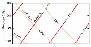
y � mx � c, where m is the same for all isothermsand c is a different constant for each isotherm.Therefore, on the skew T � ln p chart, isotherms arestraight parallel lines that slope upward from leftto right. The scale for the x axis is generally chosento make the angle between the isotherms and theisobars about 45°, as depicted schematically inFig. 3.7. Note that the isotherms on a skew T � ln pchart are intentionally “skewed” by about 45° fromtheir vertical orientation in the pseudoadiabaticchart (hence the name skew T � ln p chart). From(3.55), the equation for a dry adiabat (� constant) is
Hence, on a � ln p versus ln T chart, dry adiabatswould be straight lines. Since �ln p is the ordinate onthe skew T � ln p chart, but the abscissa is not ln T,dry adiabats on this chart are slightly curved linesthat run from the lower right to the upper left. Theangle between the isotherms and the dry adiabats ona skew T � ln p chart is approximately 90° (Fig. 3.7).Therefore, when atmospheric temperature soundingsare plotted on this chart, small differences in slope
�ln p � (constant) lnT � constant
are more apparent than they are on the pseudoadia-batic chart.
Exercise 3.5 A parcel of air has a temperature of�51 °C at the 250-hPa level. What is its potentialtemperature? What temperature will the parcelhave if it is brought into the cabin of a jet aircraftand compressed adiabatically to a cabin pressure of850 hPa?
Solution: This exercise can be solved using the skewT � ln p chart. Locate the original state of the airparcel on the chart at pressure 250 hPa and temper-ature �51 °C. The label on the dry adiabat thatpasses through this point is 60 °C, which is thereforethe potential temperature of the air.
The temperature acquired by the ambient air if itis compressed adiabatically to a pressure of 850 hPacan be found from the chart by following the dry adi-abat that passes through the point located by 250 hPaand �51 °C down to a pressure of 850 hPa and read-ing off the temperature at that point. It is 44.5 °C.(Note that this suggests that ambient air brought intothe cabin of a jet aircraft at cruise altitude has tobe cooled by about 20 °C to provide a comfortableenvironment.) �
3.5 Water Vapor in AirSo far we have indicated the presence of watervapor in the air through the vapor pressure e thatit exerts, and we have quantified its effect on thedensity of air by introducing the concept of virtualtemperature. However, the amount of water vaporpresent in a certain quantity of air may be expressedin many different ways, some of the more important
Pre
ssur
e p
(hP
a)
Temperature T (K)
θ = 100 K
θ = 200 Kθ = 300 K
θ = 400 Kθ = 500 K
10
100
200
300
400
600
800
10004003002001000
0
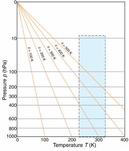
Fig. 3.6 The complete pseudoadiabatic chart. Note thatp increases downward and is plotted on a distorted scale(representing p0.286). Only the blue-shaded area is generallyprinted for use in meteorological computations. The slopinglines, each labeled with a value of the potential temperature �,are dry adiabats. As required by the definition of �, the actualtemperature of the air (given on the abscissa) at 1000 hPa isequal to its potential temperature.
Pre
ssur
e (h
Pa)
Isot
herm
T = 0
°C
T = 2
0 °C
Dry Adiabat
θ = 293 K
θ = 273 K
θ = 253 K
400
600
800
1000
T = –
20 °C
Fig. 3.7 Schematic of a portion of the skew T � ln p chart.(An accurate reproduction of a larger portion of the chart isavailable on the book web site that accompanies this book,from which it can be printed and used for solving exercises.)
p
P732951-Ch03.qxd 9/12/05 7:41 PM Page 79
3.5 Water Vapor in Air 79
y � mx � c, where m is the same for all isothermsand c is a different constant for each isotherm.Therefore, on the skew T � ln p chart, isotherms arestraight parallel lines that slope upward from leftto right. The scale for the x axis is generally chosento make the angle between the isotherms and theisobars about 45°, as depicted schematically inFig. 3.7. Note that the isotherms on a skew T � ln pchart are intentionally “skewed” by about 45° fromtheir vertical orientation in the pseudoadiabaticchart (hence the name skew T � ln p chart). From(3.55), the equation for a dry adiabat (� constant) is
Hence, on a � ln p versus ln T chart, dry adiabatswould be straight lines. Since �ln p is the ordinate onthe skew T � ln p chart, but the abscissa is not ln T,dry adiabats on this chart are slightly curved linesthat run from the lower right to the upper left. Theangle between the isotherms and the dry adiabats ona skew T � ln p chart is approximately 90° (Fig. 3.7).Therefore, when atmospheric temperature soundingsare plotted on this chart, small differences in slope
�ln p � (constant) lnT � constant
are more apparent than they are on the pseudoadia-batic chart.
Exercise 3.5 A parcel of air has a temperature of�51 °C at the 250-hPa level. What is its potentialtemperature? What temperature will the parcelhave if it is brought into the cabin of a jet aircraftand compressed adiabatically to a cabin pressure of850 hPa?
Solution: This exercise can be solved using the skewT � ln p chart. Locate the original state of the airparcel on the chart at pressure 250 hPa and temper-ature �51 °C. The label on the dry adiabat thatpasses through this point is 60 °C, which is thereforethe potential temperature of the air.
The temperature acquired by the ambient air if itis compressed adiabatically to a pressure of 850 hPacan be found from the chart by following the dry adi-abat that passes through the point located by 250 hPaand �51 °C down to a pressure of 850 hPa and read-ing off the temperature at that point. It is 44.5 °C.(Note that this suggests that ambient air brought intothe cabin of a jet aircraft at cruise altitude has tobe cooled by about 20 °C to provide a comfortableenvironment.) �
3.5 Water Vapor in AirSo far we have indicated the presence of watervapor in the air through the vapor pressure e thatit exerts, and we have quantified its effect on thedensity of air by introducing the concept of virtualtemperature. However, the amount of water vaporpresent in a certain quantity of air may be expressedin many different ways, some of the more important
Pre
ssur
e p
(hP
a)
Temperature T (K)
θ = 100 K
θ = 200 Kθ = 300 K
θ = 400 Kθ = 500 K
10
100
200
300
400
600
800
10004003002001000
0
Fig. 3.6 The complete pseudoadiabatic chart. Note thatp increases downward and is plotted on a distorted scale(representing p0.286). Only the blue-shaded area is generallyprinted for use in meteorological computations. The slopinglines, each labeled with a value of the potential temperature �,are dry adiabats. As required by the definition of �, the actualtemperature of the air (given on the abscissa) at 1000 hPa isequal to its potential temperature.
Pre
ssur
e (h
Pa)
Isot
herm
T = 0
°C
T = 2
0 °C
Dry Adiabat
θ = 293 K
θ = 273 K
θ = 253 K
400
600
800
1000T =
–20
°CFig. 3.7 Schematic of a portion of the skew T � ln p chart.(An accurate reproduction of a larger portion of the chart isavailable on the book web site that accompanies this book,from which it can be printed and used for solving exercises.)
p
P732951-Ch03.qxd 9/12/05 7:41 PM Page 79

3.5 Water Vapor in Air 81
(a) Unsaturated (b) Saturated
Water
·· ·
··
· ··
··
·
··· ·
··
·
··
·
····
· ···
·
·
·T, e T, es
··
·
Water
Fig. 3.8 A box (a) unsaturated and (b) saturated with respectto a plane surface of pure water at temperature T. Dots repre-sent water molecules. Lengths of the arrows represent therelative rates of evaporation and condensation. The saturated(i.e., equilibrium) vapor pressure over a plane surface of purewater at temperature T is es as indicated in (b).
26 For further discussion of this and some other common misconceptions related to meteorology see C. F. Bohren’s Clouds in a Glass ofBeer, Wiley and Sons, New York, 1987.
27 As a rough rule of thumb, it is useful to bear in mind that the saturation vapor pressure roughly doubles for a 10 °C increase intemperature.
to a plane surface of pure water at temperature T, andthe pressure es that is then exerted by the water vaporis called the saturation vapor pressure over a planesurface of pure water at temperature T.
Similarly, if the water in Fig. 3.8 were replaced by aplane surface of pure ice at temperature T and therate of condensation of water vapor were equal tothe rate of evaporation of the ice, the pressure esi
exerted by the water vapor would be the saturationvapor pressure over a plane surface of pure ice at T.Because, at any given temperature, the rate of evapo-ration from ice is less than from water, es(T) � esi(T).
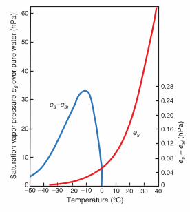
The rate at which water molecules evaporatefrom either water or ice increases with increasingtemperature.27 Consequently, both es and esi increasewith increasing temperature, and their magnitudes
depend only on temperature. The variations withtemperature of es and es � esi are shown in Fig. 3.9,where it can be seen that the magnitude of es � esi
reaches a peak value at about �12 °C. It followsthat if an ice particle is in water-saturated air it willgrow due to the deposition of water vapor upon it.In Section 6.5.3 it is shown that this phenomenon
It is common to use phrases such as “the air is sat-urated with water vapor,” “the air can hold nomore water vapor,” and “warm air can hold morewater vapor than cold air.” These phrases, whichsuggest that air absorbs water vapor, rather like asponge, are misleading. We have seen that thetotal pressure exerted by a mixture of gases isequal to the sum of the pressures that each gaswould exert if it alone occupied the total volumeof the mixture of gases (Dalton’s law of partialpressures). Hence, the exchange of water mole-
cules between its liquid and vapor phases is(essentially) independent of the presence of air.Strictly speaking, the pressure exerted by watervapor that is in equilibrium with water at a giventemperature is referred more appropriately to asequilibrium vapor pressure rather than saturationvapor pressure at that temperature. However, thelatter term, and the terms “unsaturated air” and“saturated air,” provide a convenient shorthandand are so deeply rooted that they will appear inthis book.
3.3 Can Air Be Saturated with Water Vapor?26
Temperature (°C)
es–esi
es
e s –
esi (
hPa)
0.28
0.24
0.20
0.16
0.12
0.08
0.04
0
60
50
40
30
20
10
0
Sat
urat
ion
vapo
r pr
essu
re e
s ov
er p
ure
wat
er (
hPa)
–50 403020100–10–20–30–40
Fig. 3.9 Variations with temperature of the saturation (i.e.,equilibrium) vapor pressure es over a plane surface of purewater (red line, scale at left) and the difference between es
and the saturation vapor pressure over a plane surface of iceesi (blue line, scale at right).
P732951-Ch03.qxd 9/12/05 7:41 PM Page 81
3.5 Water Vapor in Air 81
(a) Unsaturated (b) Saturated
Water
·· ·
··
· ··
··
·
··· ·
··
·
··
·
····
· ···
·
·
·T, e T, es
··
·
Water
Fig. 3.8 A box (a) unsaturated and (b) saturated with respectto a plane surface of pure water at temperature T. Dots repre-sent water molecules. Lengths of the arrows represent therelative rates of evaporation and condensation. The saturated(i.e., equilibrium) vapor pressure over a plane surface of purewater at temperature T is es as indicated in (b).
26 For further discussion of this and some other common misconceptions related to meteorology see C. F. Bohren’s Clouds in a Glass ofBeer, Wiley and Sons, New York, 1987.
27 As a rough rule of thumb, it is useful to bear in mind that the saturation vapor pressure roughly doubles for a 10 °C increase intemperature.
to a plane surface of pure water at temperature T, andthe pressure es that is then exerted by the water vaporis called the saturation vapor pressure over a planesurface of pure water at temperature T.
Similarly, if the water in Fig. 3.8 were replaced by aplane surface of pure ice at temperature T and therate of condensation of water vapor were equal tothe rate of evaporation of the ice, the pressure esi
exerted by the water vapor would be the saturationvapor pressure over a plane surface of pure ice at T.Because, at any given temperature, the rate of evapo-ration from ice is less than from water, es(T) � esi(T).
The rate at which water molecules evaporatefrom either water or ice increases with increasingtemperature.27 Consequently, both es and esi increasewith increasing temperature, and their magnitudes
depend only on temperature. The variations withtemperature of es and es � esi are shown in Fig. 3.9,where it can be seen that the magnitude of es � esi
reaches a peak value at about �12 °C. It followsthat if an ice particle is in water-saturated air it willgrow due to the deposition of water vapor upon it.In Section 6.5.3 it is shown that this phenomenon
It is common to use phrases such as “the air is sat-urated with water vapor,” “the air can hold nomore water vapor,” and “warm air can hold morewater vapor than cold air.” These phrases, whichsuggest that air absorbs water vapor, rather like asponge, are misleading. We have seen that thetotal pressure exerted by a mixture of gases isequal to the sum of the pressures that each gaswould exert if it alone occupied the total volumeof the mixture of gases (Dalton’s law of partialpressures). Hence, the exchange of water mole-
cules between its liquid and vapor phases is(essentially) independent of the presence of air.Strictly speaking, the pressure exerted by watervapor that is in equilibrium with water at a giventemperature is referred more appropriately to asequilibrium vapor pressure rather than saturationvapor pressure at that temperature. However, thelatter term, and the terms “unsaturated air” and“saturated air,” provide a convenient shorthandand are so deeply rooted that they will appear inthis book.
3.3 Can Air Be Saturated with Water Vapor?26
Temperature (°C)
es–esi
es
e s –
esi (
hPa)
0.28
0.24
0.20
0.16
0.12
0.08
0.04
0
60
50
40
30
20
10
0
Sat
urat
ion
vapo
r pr
essu
re e
s ov
er p
ure
wat
er (
hPa)
–50 403020100–10–20–30–40
Fig. 3.9 Variations with temperature of the saturation (i.e.,equilibrium) vapor pressure es over a plane surface of purewater (red line, scale at left) and the difference between es
and the saturation vapor pressure over a plane surface of iceesi (blue line, scale at right).
P732951-Ch03.qxd 9/12/05 7:41 PM Page 81

3.5 Water Vapor in Air 83
left along the 1000-hPa ordinate until we interceptthe saturation mixing ratio line of magnitude6 g kg�1; this occurs at a temperature of about 6.5 °C.Therefore, if the air is cooled at constant pressure,the water vapor it contains will just saturate the airwith respect to water at a temperature of 6.5 °C.Therefore, by definition, the dew point of the airis 6.5 °C. �
At the Earth’s surface, the pressure typically variesby only a few percent from place to place and fromtime to time. Therefore, the dew point is a good indi-cator of the moisture content of the air. In warm,humid weather the dew point is also a convenientindicator of the level of human discomfort. Forexample, most people begin to feel uncomfortablewhen the dew point rises above 20 °C, and air with adew point above about 22 °C is generally regarded asextremely humid or “sticky.” Fortunately, dew pointsmuch above this temperature are rarely observedeven in the tropics. In contrast to the dew point, rela-tive humidity depends as much upon the tempera-ture of the air as upon its moisture content. On asunny day the relative humidity may drop by asmuch as 50% from morning to afternoon, justbecause of a rise in air temperature. Neither is rela-tive humidity a good indicator of the level of humandiscomfort. For example, a relative humidity of 70%may feel quite comfortable at a temperature of 20 °C,but it would cause considerable discomfort to mostpeople at a temperature of 30 °C.
The highest dew points occur over warm bodies ofwater or vegetated surfaces from which water is evap-orating. In the absence of vertical mixing, the air justabove these surfaces would become saturated withwater vapor, at which point the dew point would bethe same as the temperature of the underlying surface.Complete saturation is rarely achieved over hot sur-faces, but dew points in excess of 25 °C are sometimesobserved over the warmest regions of the oceans.
e. Lifting condensation level
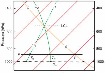
The lifting condensation level (LCL) is defined as thelevel to which an unsaturated (but moist) parcel ofair can be lifted adiabatically before it becomes satu-rated with respect to a plane surface of pure water.During lifting the mixing ratio w and potential tem-perature � of the air parcel remain constant, but thesaturation mixing ratio ws decreases until it becomesequal to w at the LCL. Therefore, the LCL is located
at the intersection of the potential temperature linepassing through the temperature T and pressure p ofthe air parcel, and the ws line that passes through thepressure p and dew point Td of the parcel (Fig. 3.10).Since the dew point and LCL are related in the man-ner indicated in Fig. 3.10, knowledge of either one issufficient to determine the other. Similarly, a knowl-edge of T, p, and any one moisture parameter is suffi-cient to determine all the other moisture parameterswe have defined.
f. Wet-bulb temperature
The wet-bulb temperature is measured with a ther-mometer, the glass bulb of which is covered with amoist cloth over which ambient air is drawn. Theheat required to evaporate water from the moistcloth to saturate the ambient air is supplied by theair as it comes into contact with the cloth. When thedifference between the temperatures of the bulb andthe ambient air is steady and sufficient to supply theheat needed to evaporate the water, the thermome-ter will read a steady temperature, which is called thewet-bulb temperature. If a raindrop falls through alayer of air that has a constant wet-bulb temperature,the raindrop will eventually reach a temperatureequal to the wet-bulb temperature of the air.
The definition of wet-bulb temperature and dewpoint both involve cooling a hypothetical air parcelto saturation, but there is a distinct difference. Ifthe unsaturated air approaching the wet bulb has amixing ratio w, the dew point Td is the temperatureto which the air must be cooled at constant pressure
C
(p, Td, ws (A))
A
θ constant
wsconstant
(p, T, w)
B
Pre
ssur
e (h
Pa)
Lifting condensation level for air at A
1000
800
600
400
Fig. 3.10 The lifting condensation level of a parcel of air atA, with pressure p, temperature T, and dew point Td, is at Con the skew T � ln p chart.
P732951-Ch03.qxd 9/12/05 7:41 PM Page 83
T
Pre
ssur
e (h
Pa)
Td
LCL
1000
800
600
400
1000
800
600
400
p
qw
wsq
ws q
Tw
qe

88 Atmospheric Thermodynamics
3.6 Static Stability3.6.1 Unsaturated Air
Consider a layer of the atmosphere in which theactual temperature lapse rate � (as measured, forexample, by a radiosonde) is less than the dry adia-batic lapse rate �d (Fig. 3.12a). If a parcel of unsat-urated air originally located at level O is raised tothe height defined by points A and B, its tempera-ture will fall to TA, which is lower than the ambienttemperature TB at this level. Because the parcelimmediately adjusts to the pressure of the ambientair, it is clear from the ideal gas equation that thecolder parcel of air must be denser than thewarmer ambient air. Therefore, if left to itself,the parcel will tend to return to its original level. Ifthe parcel is displaced downward from O itbecomes warmer than the ambient air and, if left toitself, the parcel will tend to rise back to its originallevel. In both cases, the parcel of air encounters arestoring force after being displaced, whichinhibits vertical mixing. Thus, the condition � � �d
corresponds to a stable stratification (or positivestatic stability) for unsaturated air parcels. In gen-eral, the larger the difference �d � �, the greaterthe restoring force for a given displacement and thegreater the static stability.34
Exercise 3.11 An unsaturated parcel of air has den-sity � and temperature T, and the density and tem-perature of the ambient air are � and T. Derive anexpression for the upward acceleration of the air par-cel in terms of T, T, and �.
Solution: The situation is depicted in Fig. 3.13. Ifwe consider a unit volume of the air parcel, its massis �. Therefore, the downward force acting on unitvolume of the parcel is ��. From the Archimedes35
principle we know that the upward force acting onthe parcel is equal in magnitude to the gravitationalforce that acts on the ambient air that is displaced bythe air parcel. Because a unit volume of ambient airof density � is displaced by the air parcel, the magni-tude of the upward force acting on the air parcel is��. Therefore, the net upward force (F) acting on aunit volume of the parcel is
F � (� � �) �
34 A more general method for determing static stability is given in Section 9.3.4.35 Archimedes (287–212 B.C.) The greatest of Greek scientists. He invented engines of war and the water screw and he derived the
principle of buoyancy named after him. When Syracuse was sacked by Rome, a soldier came upon the aged Archimedes absorbed in study-ing figures he had traced in the sand: “Do not disturb my circles” said Archimedes, but was killed instantly by the soldier. Unfortunately,right does not always conquer over might.
TemperatureTATB
Hei
ght
Γd
Γ
(b)
AB
(a)Temperature
TA TB
ΓdΓ
O
BA
Hei
ght
O
Fig. 3.12 Conditions for (a) positive static stability (� � �d)and (b) negative static instability (� � �d) for the displace-ment of unsaturated air parcels.
Fig. 3.13 The box represents an air parcel of unit volumewith its center of mass at height z above the Earth’s surface.The density and temperature of the air parcel are � and T,respectively, and the density and temperature of the ambientair are � and T. The vertical forces acting on the air parcel areindicated by the thicker arrows.
ρg
Surface
ρ′g
ρ, T ρ′, T ′
z
P732951-Ch03.qxd 9/12/05 7:41 PM Page 88

90 Atmospheric Thermodynamics
mountainous terrain, as shown in the top photographin Fig. 3.14 or by an intense local disturbance, asshown in the bottom photograph. The following exer-cise illustrates how buoyancy oscillations can beexcited by flow over a mountain range.
Exercise 3.13 A layer of unsaturated air flows overmountainous terrain in which the ridges are 10 kmapart in the direction of the flow. The lapse rate is 5 °Ckm�1 and the temperature is 20 °C. For what value ofthe wind speed U will the period of the orographic(i.e., terrain-induced) forcing match the period of abuoyancy oscillation?
Solution: For the period � of the orographic forcingto match the period of the buoyancy oscillation, it isrequired that
where L is the spacing between the ridges. Hence,from this last expression and (3.75),
or, in SI units,
�
Layers of air with negative lapse rates (i.e., tempera-tures increasing with height) are called inversions. Itis clear from the aforementioned discussion thatthese layers are marked by very strong static stabil-ity. A low-level inversion can act as a “lid” that trapspollution-laden air beneath it (Fig. 3.15). The layeredstructure of the stratosphere derives from the factthat it represents an inversion in the vertical temper-ature profile.
If � � �d (Fig. 3.12b), a parcel of unsaturated airdisplaced upward from O will arrive at A with a tem-perature greater than that of its environment.Therefore, it will be less dense than the ambient air
� 20 m s�1
U �104
2� �9.8
293 (9.8 � 5.0) � 10�3�1/2
U �LN2�
�L2�
��T
(�d � �)�1/2
� �LU
�2�
N
Fig. 3.14 Gravity waves, as revealed by cloud patterns.The upper photograph, based on NOAA GOES 8 visiblesatellite imagery, shows a wave pattern in west to east(right to left) airflow over the north–south-oriented moun-tain ranges of the Appalachians in the northeastern UnitedStates. The waves are transverse to the flow and their hori-zontal wavelength is �20 km. The atmospheric wave pat-tern is more regular and widespread than the undulationsin the terrain. The bottom photograph, based on imageryfrom NASA’s multiangle imaging spectro-radiometer(MISR), shows an even more regular wave pattern in a thinlayer of clouds over the Indian Ocean.
Fig. 3.15 Looking down onto widespread haze over south-ern Africa during the biomass-burning season. The haze isconfined below a temperature inversion. Above the inversion,the air is remarkably clean and the visibility is excellent.(Photo: P. V. Hobbs.)
P732951-Ch03.qxd 9/12/05 7:41 PM Page 90

3.6 Static Stability 91
and, if left to itself, will continue to rise. Similarly, ifthe parcel is displaced downward it will be coolerthan the ambient air, and it will continue to sink ifleft to itself. Such unstable situations generally do notpersist in the free atmosphere, because the instabilityis eliminated by strong vertical mixing as fast as itforms. The only exception is in the layer just abovethe ground under conditions of very strong heatingfrom below. �
Exercise 3.14 Show that if the potential tempera-ture � increases with increasing altitude the atmos-phere is stable with respect to the displacement ofunsaturated air parcels.
Solution: Combining (3.1), (3.18), and (3.67), weobtain for a unit mass of air
Letting d� � (����z)dz and dT � (�T��z)dz anddividing through by cpTdz yields
(3.76)
Noting that �dT�dz is the actual lapse rate � of theair and the dry adiabatic lapse rate �d is ��cp (3.76)may be written as
(3.77)
However, it has been shown earlier that when � � �d
the air is characterized by positive static stability. Itfollows that under these same conditions ����z mustbe positive; that is, the potential temperature mustincrease with height. �
3.6.2 Saturated Air
If a parcel of air is saturated, its temperature willdecrease with height at the saturated adiabatic lapserate �s. It follows from arguments similar to thosegiven in Section 3.6.1 that if � is the actual lapse rateof temperature in the atmosphere, saturated airparcels will be stable, neutral, or unstable withrespect to vertical displacements, depending onwhether � � �s, � � �s, or � � �s, respectively. When
1� ��
�z�
1T
(�d � �)
1� ��
�z�
1T
�T�z
��cp
cpT d�
�� cp dT � �dz
an environmental temperature sounding is plottedon a skew T � ln p chart the distinctions between �,�d, and �s are clearly discernible (see Exercise 3.53).
3.6.3 Conditional and Convective Instability
If the actual lapse rate � of the atmosphere liesbetween the saturated adiabatic lapse rate �s and thedry adiabatic lapse rate �d, a parcel of air that islifted sufficiently far above its equilibrium level willbecome warmer than the ambient air. This situationis illustrated in Fig. 3.16, where an air parcel liftedfrom its equilibrium level at O cools dry adiabaticallyuntil it reaches its lifting condensation level at A. Atthis level the air parcel is colder than the ambient air.Further lifting produces cooling at the moist adia-batic lapse rate so the temperature of the parcel ofair follows the moist adiabat ABC. If the air parcel issufficiently moist, the moist adiabat through A willcross the ambient temperature sounding; the point ofintersection is shown as B in Fig. 3.16. Up to thispoint the parcel was colder and denser than theambient air, and an expenditure of energy wasrequired to lift it. If forced lifting had stopped priorto this point, the parcel would have returned to itsequilibrium level at point O. However, once abovepoint B, the parcel develops a positive buoyancy thatcarries it upward even in the absence of furtherforced lifting. For this reason, B is referred to as thelevel of free convection (LFC). The level of free con-vection depends on the amount of moisture in therising parcel of air, as well as the magnitude of thelapse rate �.
From the aforementioned discussion it is clear thatfor a layer in which �s � � � �d, vigorous convectiveoverturning will occur if forced vertical motions are
B
OA
Γ
Hei
ght
LFC
LCL
Γs Γd
Temperature
Fig. 3.16 Conditions for conditional instability (�s � � �
�d). �s and �d are the saturated and dry adiabatic lapse rates,and � is the lapse rate of temperature of the ambient air. LCLand LFC denote the lifting condensation level and the level of freeconvection, respectively.
P732951-Ch03.qxd 9/12/05 7:41 PM Page 91
92 Atmospheric Thermodynamics
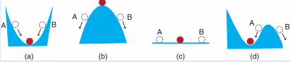
Sections 3.6.1 and 3.6.2 discussed the conditionsfor parcels of unsaturated air and saturated air tobe stable, unstable, or neutral when displaced ver-tically in the atmosphere. Under stable conditions,if an air parcel is displaced either upward ordownward and is then left to itself (i.e., the forcecausing the original displacement is removed), theparcel will return to its original position. An anal-ogous situation is shown in Fig. 3.17a where a ballis originally located at the lowest point in a valley.If the ball is displaced in any direction and is thenleft to itself, it will return to its original location atthe base of the valley.
Under unstable conditions in the atmosphere, anair parcel that is displaced either upward or down-ward, and then left to itself, will continue to moveupward or downward, respectively. An analog isshown in Fig. 3.17b, where a ball is initially on topof a hill. If the ball is displaced in any direction,and is then left to itself, it will roll down the hill.
If an air parcel is displaced in a neutral atmos-phere, and then left to itself, it will remain in thedisplaced location. An analog of this condition isa ball on a flat surface (Fig. 3.17c). If the ball isdisplaced, and then left to itself, it will not move.
If an air parcel is conditionally unstable, it canbe lifted up to a certain height and, if left toitself, it will return to its original location.However, if the air parcel is lifted beyond a cer-tain height (i.e., the level of free convection), andis then left to itself, it will continue rising(Section 3.6.3). An analog of this situation isshown in Fig. 3.17d, where a displacement of aball to a point A, which lies to the left of thehillock, will result in the ball rolling back to itsoriginal position. However, if the displacementtakes the ball to a point B on the other side ofthe hillock, the ball will not return to its originalposition but will roll down the right-hand side ofthe hillock.
It should be noted that in the analogs shownin Fig. 3.17 the only force acting on the ball afterit is displaced is that due to gravity, which isalways downward. In contrast, an air parcel isacted on by both a gravitational force and abuoyancy force. The gravitational force is alwaysdownward. The buoyancy force may be eitherupward or downward, depending on whether theair parcel is less dense or more dense than theambient air.
3.4 Analogs for Static Stability, Instability, Neutral Stability, and Conditional Instability
(a) (b) (c)
BA
AB
A BA B
(d)
Fig. 3.17 Analogs for (a) stable, (b) unstable, (c) neutral, and (d) conditional instability. The red circle is the originalposition of the ball, and the white circles are displaced positions. Arrows indicate the direction the ball will move from adisplaced position if the force that produced the displacement is removed.
large enough to lift air parcels beyond their level offree convection. Such an atmosphere is said to beconditionally unstable with respect to convection. Ifvertical motions are weak, this type of stratificationcan be maintained indefinitely.
The potential for instability of air parcels is alsorelated to the vertical stratification of water vapor. Inthe profiles shown in Fig. 3.18, the dew pointdecreases rapidly with height within the inversionlayer AB that marks the top of a moist layer. Now,
suppose that this layer is lifted. An air parcel at Awill reach its LCL quickly, and beyond that point itwill cool moist adiabatically. In contrast, an air parcelstarting at point B will cool dry adiabatically througha deep layer before it reaches its LCL. Therefore, asthe inversion layer is lifted, the top part of it coolsmuch more rapidly than the bottom part, and thelapse rate quickly becomes destabilized. Sufficientlifting may cause the layer to become conditionallyunstable, even if the entire sounding is absolutely
P732951-Ch03.qxd 9/12/05 7:41 PM Page 92

3.7 The Second Law of Thermodynamics and Entropy 93
stable to begin with. It may be shown that the criterionfor this so-called convective (or potential) instabilityis that ��e��z be negative (i.e., �e decrease withincreasing height) within the layer.
Throughout large areas of the tropics, �e decreasesmarkedly with height from the mixed layer to themuch drier air above. Yet deep convection breaks outonly within a few percent of the area where there issufficient lifting to release the instability.
3.7 The Second Law ofThermodynamics and EntropyThe first law of thermodynamics (Section 3.3) is astatement of the principle of conservation of energy.The second law of thermodynamics, which wasdeduced in various forms by Carnot,38 Clausius,39
and Lord Kelvin, is concerned with the maximumfraction of a quantity of heat that can be convertedinto work. The fact that for any given system there isa theoretical limit to this conversion was first clearlydemonstrated by Carnot, who also introduced theimportant concepts of cyclic and reversible processes.
3.7.1 The Carnot Cycle
A cyclic process is a series of operations by whichthe state of a substance (called the working sub-stance) changes but the substance is finally returnedto its original state in all respects. If the volumeof the working substance changes, the working sub-
stance may do external work, or work may be doneon the working substance, during a cyclic process.Since the initial and final states of the working sub-stance are the same in a cyclic process, and internalenergy is a function of state, the internal energy ofthe working substance is unchanged in a cyclicprocess. Therefore, from (3.33), the net heatabsorbed by the working substance is equal to theexternal work that it does in the cycle. A workingsubstance is said to undergo a reversible transforma-tion if each state of the system is in equilibrium sothat a reversal in the direction of an infinitesimalchange returns the working substance and the envi-ronment to their original states. A heat engine (orengine for short) is a device that does work throughthe agency of heat.
If during one cycle of an engine a quantity of heatQ1 is absorbed and heat Q2 is rejected, the amount ofwork done by the engine is Q1 � Q2 and its efficiency� is defined as
(3.78)
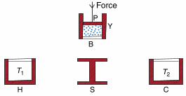
Carnot was concerned with the important practicalproblem of the efficiency with which heat enginescan do useful mechanical work. He envisaged anideal heat engine (Fig. 3.19) consisting of a workingsubstance contained in a cylinder (Y) with insulatingwalls and a conducting base (B) that is fitted with aninsulated, frictionless piston (P) to which a variableforce can be applied, a nonconducting stand (S) onwhich the cylinder may be placed to insulate its base,an infinite warm reservoir of heat (H) at constanttemperature T1, and an infinite cold reservoir forheat (C) at constant temperature T2 (where T1 � T2).Heat can be supplied from the warm reservoir to theworking substance contained in the cylinder, andheat can be extracted from the working substance bythe cold reservoir. As the working substance expands(or contracts), the piston moves outward (or inward)and external work is done by (or on) the workingsubstance.
�Q1 � Q2
Q1
� �Work done by the engine
Heat absorbed by the working substance
BA
Td T
Hei
ght
Temperature
Fig. 3.18 Conditions for convective instability. T and Td arethe temperature and dew point of the air, respectively. Theblue-shaded region is a dry inversion layer.
38 Nicholas Leonard Sadi Carnot (1796–1832) Born in Luxenbourg. Admitted to the École Polytechnique, Paris, at age 16. Became acaptain in the Corps of Engineers. Founded the science of thermodynamics.
39 Rudolf Clausius (1822–1888) German physicist. Contributed to the sciences of thermodynamics, optics, and electricity.
P732951-Ch03.qxd 9/12/05 7:41 PM Page 93
94 Atmospheric Thermodynamics
Carnot’s cycle consists of taking the working sub-stance in the cylinder through the following fouroperations that together constitute a reversible, cyclictransformation:
i. The substance starts with temperature T2 at acondition represented by A on the p–V diagramin Fig. 3.20. The cylinder is placed on the standS and the working substance is compressed byincreasing the downward force applied to thepiston. Because heat can neither enter norleave the working substance in the cylinderwhen it is on the stand, the working substanceundergoes an adiabatic compression to thestate represented by B in Fig. 3.20 in which itstemperature has risen to T1.
ii. The cylinder is now placed on the warmreservoir H, from which it extracts a quantity ofheat Q1. During this process the workingsubstance expands isothermally at temperatureT1 to point C in Fig. 3.20. During this processthe working substance does work by expandingagainst the force applied to the piston.
iii. The cylinder is returned to the nonconductingstand and the working substance undergoes anadiabatic expansion along book web site inFig. 3.20 until its temperature falls to T2.Again the working substance does workagainst the force applied to the piston.
iv. Finally, the cylinder is placed on the coldreservoir and, by increasing the force appliedto the piston, the working substance iscompressed isothermally along DA back to itsoriginal state A. In this transformation theworking substance gives up a quantity of heatQ2 to the cold reservoir.
It follows from (3.36) that the net amount of workdone by the working substance during the Carnotcycle is equal to the area contained within the figureABCD in Fig. 3.20. Also, because the working sub-stance is returned to its original state, the net workdone is equal to Q1 � Q2 and the efficiency of theengine is given by (3.78). In this cyclic operation theengine has done work by transferring a certain quan-tity of heat from a warmer (H) to a cooler (C) body.One way of stating the second law of thermodynam-ics is “only by transferring heat from a warmer to acolder body can heat be converted into work in acyclic process.” In Exercise 3.56 we prove that noengine can be more efficient than a reversible engineworking between the same limits of temperature, andthat all reversible engines working between the sametemperature limits have the same efficiency. The valid-ity of these two statements, which are known asCarnot’s theorems, depends on the truth of the sec-ond law of thermodynamics.
Exercise 3.15 Show that in a Carnot cycle theratio of the heat Q1 absorbed from the warm reser-voir at temperature T1 K to the heat Q2 rejectedto the cold reservoir at temperature T2 K is equalto T1�T2.
Solution: To prove this important relationship welet the substance in the Carnot engine be 1 mol of anideal gas and we take it through the Carnot cycleABCD shown in Fig. 3.20.
For the adiabatic transformation of the ideal gasfrom A to B we have (using the adiabatic equationthat the reader is invited to prove in Exercise 3.33)
where � is the ratio of the specific heat at constantpressure to the specific heat at constant volume. For
pA V�A
� pBV�B
Force
PY
B
SH C
T2T1
Fig. 3.19 The components of Carnot’s ideal heat engine.Red-shaded areas indicate insulating material, and whiteareas represent thermally conducting material. The workingsubstance is indicated by the blue dots inside the cylinder.
T1 Isotherm
T2 Isotherm
B
C
D
A
AdiabatAdiabat
Pre
ssur
e
Volume
Fig. 3.20 Representations of a Carnot cycle on a p–V dia-gram. Red lines are isotherms, and orange lines are adiabats.
P732951-Ch03.qxd 9/12/05 7:41 PM Page 94

96 Atmospheric Thermodynamics
In passing reversibly from one adiabat to anotheralong an isotherm (e.g., in one operation of a Carnotcycle) heat is absorbed or rejected, where theamount of heat Qrev (the subscript “rev” indicatesthat the heat is exchanged reversibly) depends onthe temperature T of the isotherm. Moreover, it fol-lows from (3.83) that the ratio Qrev�T is the same nomatter which isotherm is chosen in passing from oneadiabat to another. Therefore, the ratio Qrev�T couldbe used as a measure of the difference between thetwo adiabats; Qrev�T is called the difference inentropy (S) between the two adiabats. More pre-cisely, we may define the increase in the entropy dSof a system as
(3.84)
where dQrev is the quantity of heat that is addedreversibly to the system at temperature T. For a unitmass of the substance
(3.85)
Entropy is a function of the state of a system and notthe path by which the system is brought to that state.We see from (3.38) and (3.85) that the first law ofthermodynamics for a reversible transformation maybe written as
(3.86)
In this form the first law contains functions of stateonly.
Tds � du � pd�
ds � dqrev
T
dS � dQrev
T
When a system passes from state 1 to state 2, thechange in entropy of a unit mass of the system is
(3.87)
Combining (3.66) and (3.67) we obtain
(3.88)
Therefore, because the processes leading to (3.66)and (3.67) are reversible, we have from (3.85) and(3.88)
(3.89)
Integrating (3.89) we obtain the relationship betweenentropy and potential temperature
(3.90)
Transformations in which entropy (and thereforepotential temperature) is constant are called isen-tropic. Therefore, adiabats are often referred to asisentropies in atmospheric science. We see from(3.90) that the potential temperature can be used asa surrogate for entropy, as is generally done inatmospheric science.
Let us consider now the change in entropy in theCarnot cycle shown in Fig. 3.20. The transformationsfrom A to B and from C to D are both adiabatic andreversible; therefore, in these two transformationsthere can be no changes in entropy. In passing fromstate B to state C, the working substance takes in aquantity of heat Q1 reversibly from the source at tem-perature T1; therefore, the entropy of the sourcedecreases by an amount Q1�T1. In passing from stateD to state A, a quantity of heat Q2 is rejectedreversibly from the working substance to the sink attemperature T2; therefore, the entropy of the sinkincreases by Q2�T2. Since the working substance itselfis taken in a cycle, and is therefore returned to itsoriginal state, it does not undergo any net change inentropy. Therefore, the net increase in entropy in thecomplete Carnot cycle is Q2�T2 � Q1�T1. However,we have shown in Exercise 3.15 that Q1�T1 � Q2�T2.Hence, there is no change in entropy in a Carnotcycle.
s � cp ln � � constant
ds � cpd�
�
dqT
� cpd�
�
s2 � s1 � �2
1 dqrev
TT1
T2
T3
θ1 θ2 θ3
Volume
Pre
ssur
e
Fig. 3.21 Isotherms (red curves labeled by temperature T)and adiabats (tan curves labeled by potential temperature �)on a p–V diagram.
P732951-Ch03.qxd 9/12/05 7:41 PM Page 96

3.7 The Second Law of Thermodynamics and Entropy 97
It is interesting to note that if, in a graph (called atemperature–entropy diagram40), temperature (in kelvin)is taken as the ordinate and entropy as the abscissa, theCarnot cycle assumes a rectangular shape, as shown inFig. 3.22 where the letters A, B, C, and D correspond tothe state points in the previous discussion. Adiabaticprocesses (AB and CD) are represented by verticallines (i.e., lines of constant entropy) and isothermalprocesses (BC and DA) by horizontal lines. From (3.84)it is evident that in a cyclic transformation ABCDA, theheat Q1 taken in reversibly by the working substancefrom the warm reservoir is given by the area XBCY,and the heat Q2 rejected by the working substance tothe cold reservoir is given by the area XADY.Therefore, the work Q1 � Q2 done in the cycle isgiven by the difference between the two areas, which isequivalent to the shaded area ABCD in Fig. 3.22.Any reversible heat engine can be represented by aclosed loop on a temperature–entropy diagram, and thearea of the loop is proportional to the net work done byor on (depending on whether the loop is traversedclockwise or counterclockwise, respectively) the enginein one cycle.
Thermodynamic charts on which equal areas rep-resent equal net work done by or on the workingsubstance are particularly useful. The skew T � ln pchart has this property.
3.7.3 The Clausius–Clapeyron Equation
We will now utilize the Carnot cycle to derive animportant relationship, known as the Clausius–Clapeyron42 equation (sometimes referred to byphysicists as the first latent heat equation). TheClausius–Clapeyron equation describes how thesaturated vapor pressure above a liquid changeswith temperature and also how the melting point ofa solid changes with pressure.
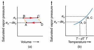
Let the working substance in the cylinder of aCarnot ideal heat engine be a liquid in equilibriumwith its saturated vapor and let the initial state of thesubstance be represented by point A in Fig. 3.23 inwhich the saturated vapor pressure is es � des at tem-perature T � dT. The adiabatic compression fromstate A to state B, where the saturated vapor pres-sure is es at temperature T, is achieved by placing thecylinder on the nonconducting stand and compress-ing the piston infinitesimally (Fig. 3.24a). Now let thecylinder be placed on the source of heat at tempera-ture T and let the substance expand isothermallyuntil a unit mass of the liquid evaporates (Fig. 3.24b).
40 The temperature–entropy diagram was introduced into meteorology by Shaw.41 Because entropy is sometimes represented by thesymbol � (rather than S), the temperature–entropy diagram is sometimes referred to as a tephigram.
41 Sir (William) Napier Shaw (1854–1945) English meteorologist. Lecturer in Experimental Physics, Cambridge University, 1877–1899.Director of the British Meteorological Office, 1905–1920. Professor of Meteorology, Imperial College, University of London, 1920–1924.Shaw did much to establish the scientific basis of meteorology. His interests ranged from the atmospheric general circulation and forecast-ing to air pollution.
42 Benoit Paul Emile Clapeyron (1799–1864) French engineer and scientist. Carnot’s theory of heat engines was virtually unknownuntil Clapeyron expressed it in analytical terms. This brought Carnot’s ideas to the attention of William Thomson (Lord Kelvin) andClausius, who utilized them in formulating the second law of thermodynamics.
Fig. 3.22 Representation of the Carnot cycle on a tempera-ture (T)–entropy (S) diagram. AB and CD are adiabats, andBC and DA are isotherms.
Fig. 3.23 Representation on (a) a saturated vapor pressureversus volume diagram and on (b) a saturated vapor pressureversus temperature diagram of the states of a mixture of aliquid and its saturated vapor taken through a Carnot cycle.Because the saturated vapor pressure is constant if tempera-ture is constant, the isothermal transformations BC and DAare horizontal lines.
T1
T2
A
X Y
D
Adiabat Adiabat
Isotherm
Isotherm
Tem
pera
ture
, T
Entropy, S
B C
es
es – des
B C
DA
Sat
urat
ed v
apor
pre
ssur
e
Sat
urat
ed v
apor
pre
ssur
e
es – des
es
A, D
B, C
T – dT T
(b)
Temperature
(a)
Volume
P732951-Ch03.qxd 9/12/05 7:41 PM Page 97
3.7 The Second Law of Thermodynamics and Entropy 97
It is interesting to note that if, in a graph (called atemperature–entropy diagram40), temperature (in kelvin)is taken as the ordinate and entropy as the abscissa, theCarnot cycle assumes a rectangular shape, as shown inFig. 3.22 where the letters A, B, C, and D correspond tothe state points in the previous discussion. Adiabaticprocesses (AB and CD) are represented by verticallines (i.e., lines of constant entropy) and isothermalprocesses (BC and DA) by horizontal lines. From (3.84)it is evident that in a cyclic transformation ABCDA, theheat Q1 taken in reversibly by the working substancefrom the warm reservoir is given by the area XBCY,and the heat Q2 rejected by the working substance tothe cold reservoir is given by the area XADY.Therefore, the work Q1 � Q2 done in the cycle isgiven by the difference between the two areas, which isequivalent to the shaded area ABCD in Fig. 3.22.Any reversible heat engine can be represented by aclosed loop on a temperature–entropy diagram, and thearea of the loop is proportional to the net work done byor on (depending on whether the loop is traversedclockwise or counterclockwise, respectively) the enginein one cycle.
Thermodynamic charts on which equal areas rep-resent equal net work done by or on the workingsubstance are particularly useful. The skew T � ln pchart has this property.
3.7.3 The Clausius–Clapeyron Equation
We will now utilize the Carnot cycle to derive animportant relationship, known as the Clausius–Clapeyron42 equation (sometimes referred to byphysicists as the first latent heat equation). TheClausius–Clapeyron equation describes how thesaturated vapor pressure above a liquid changeswith temperature and also how the melting point ofa solid changes with pressure.
Let the working substance in the cylinder of aCarnot ideal heat engine be a liquid in equilibriumwith its saturated vapor and let the initial state of thesubstance be represented by point A in Fig. 3.23 inwhich the saturated vapor pressure is es � des at tem-perature T � dT. The adiabatic compression fromstate A to state B, where the saturated vapor pres-sure is es at temperature T, is achieved by placing thecylinder on the nonconducting stand and compress-ing the piston infinitesimally (Fig. 3.24a). Now let thecylinder be placed on the source of heat at tempera-ture T and let the substance expand isothermallyuntil a unit mass of the liquid evaporates (Fig. 3.24b).
40 The temperature–entropy diagram was introduced into meteorology by Shaw.41 Because entropy is sometimes represented by thesymbol � (rather than S), the temperature–entropy diagram is sometimes referred to as a tephigram.
41 Sir (William) Napier Shaw (1854–1945) English meteorologist. Lecturer in Experimental Physics, Cambridge University, 1877–1899.Director of the British Meteorological Office, 1905–1920. Professor of Meteorology, Imperial College, University of London, 1920–1924.Shaw did much to establish the scientific basis of meteorology. His interests ranged from the atmospheric general circulation and forecast-ing to air pollution.
42 Benoit Paul Emile Clapeyron (1799–1864) French engineer and scientist. Carnot’s theory of heat engines was virtually unknownuntil Clapeyron expressed it in analytical terms. This brought Carnot’s ideas to the attention of William Thomson (Lord Kelvin) andClausius, who utilized them in formulating the second law of thermodynamics.
Fig. 3.22 Representation of the Carnot cycle on a tempera-ture (T)–entropy (S) diagram. AB and CD are adiabats, andBC and DA are isotherms.
Fig. 3.23 Representation on (a) a saturated vapor pressureversus volume diagram and on (b) a saturated vapor pressureversus temperature diagram of the states of a mixture of aliquid and its saturated vapor taken through a Carnot cycle.Because the saturated vapor pressure is constant if tempera-ture is constant, the isothermal transformations BC and DAare horizontal lines.
T1
T2
A
X Y
D
Adiabat Adiabat
Isotherm
Isotherm
Tem
pera
ture
, T
Entropy, S
B C
es
es – des
B C
DA
Sat
urat
ed v
apor
pre
ssur
e
Sat
urat
ed v
apor
pre
ssur
e
es – des
es
A, D
B, C
T – dT T
(b)
Temperature
(a)
Volume
P732951-Ch03.qxd 9/12/05 7:41 PM Page 97
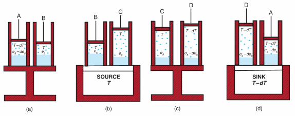
98 Atmospheric Thermodynamics
In this transformation the pressure remains constantat es and the substance passes from state B to state C(Fig. 3.24b). If the specific volumes of liquid andvapor at temperature T are �1 and �2, respectively,the increase in the volume of the system in passingfrom state B to C is (�2 � �1). Also the heatabsorbed from the source is Lv where Lv is the latentheat of vaporization. The cylinder is now placedagain on the nonconducting stand and a small adia-batic expansion is carried out from state C to state Din which the temperature falls from T to T � dT andthe pressure from es to es � des (Fig. 3.24c). Finally,the cylinder is placed on the heat sink at temperatureT � dT and an isothermal and isobaric compressionis carried out from state D to state A during whichvapor is condensed (Fig. 3.24d). All of the aforemen-tioned transformations are reversible.
From (3.83)
(3.91)
where Q1 � Q2 is the net heat absorbed by the work-ing substance in the cylinder during one cycle, whichis also equal to the work done by the working sub-stance in the cycle. However, as shown in Section 3.3,the work done during a cycle is equal to the area ofthe enclosed loop on a p–V diagram. Therefore, fromFig. 3.23, Q1 � Q2 � BC � des � (�2 � �1)des. Also,Q1 � Lv, T1 � T, and T1 � T2 � dT. Therefore, sub-stituting into (3.91),
or
Lv
T�
(�2 � �1)des
dT
Q1
T1�
Q2
T2�
Q1 � Q2
T1 � T2
(3.92)
which is the Clausius–Clapeyron equation for thevariation of the equilibrium vapor pressure es withtemperature T.
Since the volume of a unit mass of vapor is verymuch greater than the volume of a unit mass of liq-uid (�2 �� �1), Eq. (3.92) can be written to closeapproximation as
(3.93)
Because �2 is the specific volume of water vapor thatis in equilibrium with liquid water at temperature T,the pressure it exerts at T is es. Therefore, from theideal gas equation for water vapor,
(3.94)
combining (3.93) and (3.94), and then substitutingRv � 1000 R*�Mw from (3.13), we get
(3.95)
which is a convenient form of the Clausius–Clapeyron equation. Over the relatively small rangeof temperatures of interest in the atmosphere, togood approximation (3.95) can be applied in incre-mental form, that is
(3.96)1es
�es
�T�
Lv Mw
1000 R*T2
1es
des
dT�
Lv
RvT2 �LvMw
1000 R*T2
es �2 � RvT
des
dT�
Lv
T�2
des
dT�
Lv
T (�2 � �1)
T-dT
es – des
T – dT
es – deses – des
T – dT
es
T
es
T
Tes
T – dT
es – des
Tes
T – dT
(a) (b) (c) (d)
ADD
CCBBA
SOURCET
SINKT – dT
Fig. 3.24 Transformations of a liquid (solid blue) and its saturated vapor (blue dots) in a Carnot cycle. The letters A, B, C, Dindicate the states of the mixture shown in Fig. 3.23. Red-shaded areas are thermally insulating materials.
P732951-Ch03.qxd 9/12/05 7:41 PM Page 98

3.7 The Second Law of Thermodynamics and Entropy 99
Applying (3.95) to the water substance, and integrat-ing from 273 K to T K,
Alternatively, because es at 273 K � 6.11 hPa (Fig. 3.9),Lv � 2.500 � 106 J kg�1, the molecular weight of water
�es (T K)
es (273 K)
des
es�
LvMw
1000 R* �T
273 dTT2
(Mw) is 18.016, and R* � 8.3145 J K�1 mol�1, the satu-rated vapor pressure of water es (in hPa) at tempera-ture T K is given by
(3.97)� 5.42 � 103 1273
�1T
ln es (in hPa)
6.11�
LvMw
1000 R* 1273
�1T
43 If, as is generally the case, the water is in a vessel that is heated from below, the pressure where the bubbles originate is slightly greaterthan atmospheric pressure due to the extra pressure exerted by the water above the bubble. Therefore, when the water is boiling steadily, thetemperature at the bottom of the vessel will be slightly in excess of TB. When water is heated in a transparent vessel, the first visible sign ofbubbling occurs well below TB as trains of small bubbles of dissolved air rise to the surface. (Note: the solubility of a gas in a liquid decreaseswith increasing temperature.) The “singing” that precedes boiling is due to the collapse of bubbles of water vapor in the upper part of the ves-sel. Those vapor bubbles probably form around air bubbles that act as nuclei, which originate in the slightly hotter water nearer the source ofthe heat. Nuclei of some sort appear to be necessary for continuous steady boiling at TB.Without nuclei the water will not begin to boil until itis superheated with respect to the boiling point and “bumping” (i.e., delayed boiling) occurs. When bubbles finally form, the vapor pressure inthe bubbles is much greater than the ambient pressure, and the bubbles expand explosively as they rise. Chapter 6 discusses the formation ofwater drops from the vapor phase, and ice particles from the vapor and liquid phases both of which require nucleation.
A liquid is said to boil when it is heated to a temper-ature that is sufficient to produce copious smallbubbles within the liquid. Why do bubbles form at acertain temperature (the boiling point) for each liq-uid? The key to the answer to this question is torealize that if a bubble forms in a liquid, the interiorof the bubble contains only the vapor of the liquid.Therefore, the pressure inside the bubble is the satu-ration vapor pressure at the temperature of the liq-uid. If the saturation vapor pressure is less than theambient pressure that acts on the liquid (and there-fore on a bubble just below the surface of a liquid),bubbles cannot form. As the temperature increases,the saturation vapor pressure increases (see Fig. 3.9)and, when the saturation vapor pressure is equal tothe ambient pressure, bubbles can form at the sur-face of the liquid and the liquid boils (Fig. 3.25).
Water boils at a temperature TB such that thesaturation vapor pressure at TB is equal to theatmospheric (or ambient) pressure (patmos)43
(3.98)
From (3.92) expressed in incremental form, and(3.98)
�patmos
∆TB�
Lv
TB (�2 � �1)
es(TB) � patmos
or
(3.99)
Equation (3.99) gives the change in the boilingpoint of water with atmospheric pressure (orambient pressure in general). Because �2 � �1, TB
increases with increasing patmos. If the atmosphericpressure is significantly lower than 1 atm, the boil-ing point of water will be significantly lower than100 °C. This is why it is difficult to brew a goodcup of hot tea on top of a high mountain (seeExercise 3.64)!
�TB
∆patmos�
TB (�2 � �1)Lv
3.5 Effect of Ambient Pressure on the Boiling Point of a Liquid
(a) (b)
patmos patmos
Pressureinsidebubble =es(TB) = patmos
T < TBWater
T = TBWater
Fig. 3.25 (a) Water below its boiling point (TB): bubblescannot form because es(T) � patmos. (b) Water at its boil-ing point: bubbles can form because the pressure insidethem, es(TB), is equal to the atmospheric pressure (patmos)acting on them.
P732951-Ch03.qxd 9/12/05 7:41 PM Page 99
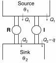
Exercises 109
temperature. Suppose initially that I ismore efficient than R and use I to drive Rbackward. Show that this leads to aviolation of the second law ofthermodynamics, and hence prove that Icannot be more efficient than R.]
(b) All reversible engines working between thesame limits of temperature have the sameefficiency. [Hint: Proof is similar to that forpart (a).]
Solution:
(a) To prove that no engine can be more efficientthan a reversible engine working betweenthe same limits of temperature, consider areversible (R) and irreversible (I) engineworking between �1 and �2.Assume I is moreefficient than R and that R takes heatQ1 from source and yields heat Q2 to sink(Fig. 3.26).Therefore, if I takes Q1 fromsource it must yield heat Q2 � q (q positive)to sink. Now let us use I to drive R backward.This will require I to do work Q1 � Q2 on R.However, in one cycle, I develops work Q1 � (Q2 � q) � (Q1 � Q2) � q. Hence,even when I is drawing R backward,mechanical work q is still available. However,in one cycle of the combined system, heat Q2 � (Q2 � q) � q is taken from a colderbody. Because this violates the second law ofthermodynamics, I cannot be more efficientthan R.
(b) Take two reversible engines operatingbetween �1 and �2 and assume one engine ismore efficient than the other.Then, followingsame procedure as in (a), it can be shown thatif one reversible engine is more efficient thananother the second law is violated. �
3.57 Lord Kelvin introduced the concept of availableenergy, which he defined as the maximumamount of heat that can be converted into workby using the coldest available body in a system asthe sink for an ideal heat engine. By consideringan ideal heat engine that uses the coldestavailable body as a sink, show that the availableenergy of the universe is tending to zero and that
loss of available energy � T0 (increase inentropy)
where T0 is the temperature of the coldestavailable body.
Solution: For an ideal reversible engine
Work done in 1 cycle �
If an engine operates with sink at T0 (� T2):
Available energy =
Let Q pass from T1 to T2 (T1 � T2) by, say, con-duction or radiation. Then,
Loss of available energy
Because T1 > T2, there is a loss of availableenergy for natural processes
Loss of available energy
�
3.58 An ideal reversible engine has a source and sinkat temperatures of 100 and 0 °C, respectively. Ifthe engine receives 20 J of heat from the sourcein every cycle, calculate the work done by theengine in 10 cycles. How much heat does theengine reject to the sink in 10 cycles?
3.59 A refrigerator has an internal temperature of0 °C and is situated in a room with a steady
� T0 (increase in entropy)
� T0QT2
�QT1
� QT0T1 � T2
T1T2
� T1 � T0
T1Q � T2 � T0
T2Q
T1 � T0
T1Q1
Q1 � Q2 �T1 � T2
T1Q1.
Q1 � Q2
Q1�
T1 � T2
T1
Q1 Q1
Q2 Q2 – q
R I
Sourceθ 1
Sinkθ 2
Fig. 3.26
P732951-Ch03.qxd 9/12/05 7:41 PM Page 109