Lecture 3 : Solving Equations, Curve Fitting,and Numerical Techniques

6.057 Introduction to MATLAB

Orhan Celiker

IAP 2019

1

Outline

(1) Linear Algebra(2) Polynomials(3) Optimization(4) Differentiation/Integration(5) Differential Equations

2

Systems of Linear Equations

• Given a system of linear equations➢ x+2y-3z=5➢ -3x-y+z=-8➢ x-y+z=0

MATLAB makes linearalgebra fun!

• Construct matrices so the system is described by Ax=b» A=[1 2 -3;-3 -1 1;1 -1 1];» b=[5;-8;0];

• And solve with a single line of code!» x=A\b;

➢ x is a 3x1 vector containing the values of x, y, and z

• The \ will work with square or rectangular systems.• Gives least squares solution for rectangular systems. Solution

depends on whether the system is over or underdetermined.

3

Worked Example: Linear Algebra

• Solve the following systems of equations:

➢ System 1: » A=[1 4;-3 1];» b=[34;2];» rank(A)» x=inv(A)*b;» x=A\b;

➢ System 2: » A=[2 -2;-1 1;3 4];» b=[4;3;2];» rank(A)➢ rectangular matrix

» x=A\b;➢ gives least squares solution

» error=abs(A*x1-b)4

More Linear Algebra

• Given a matrix» mat=[1 2 -3;-3 -1 1;1 -1 1];

• Calculate the rank of a matrix» r=rank(mat);

➢ the number of linearly independent rows or columns• Calculate the determinant

» d=det(mat);➢ mat must be square; matrix invertible if det nonzero

• Get the matrix inverse» E=inv(mat);

➢ if an equation is of the form A*x=b with A a square matrix,x=A\b is (mostly) the same as x=inv(A)*b

• Get the condition number» c=cond(mat); (or its reciprocal: c = rcond(mat);)

➢ if condition number is large, when solving A*x=b,small errors in b can lead to large errors in x (optimal c==1)

5

Matrix Decompositions

• MATLAB has many built-in matrix decomposition methods

• The most common ones are» [V,D]=eig(X)➢ Eigenvalue decomposition

» [U,S,V]=svd(X)➢ Singular value decomposition

» [Q,R]=qr(X)➢ QR decomposition

» [L,U]=lu(X)➢ LU decomposition

» R=chol(X)➢ Cholesky decomposition (R must be positive definite)

6

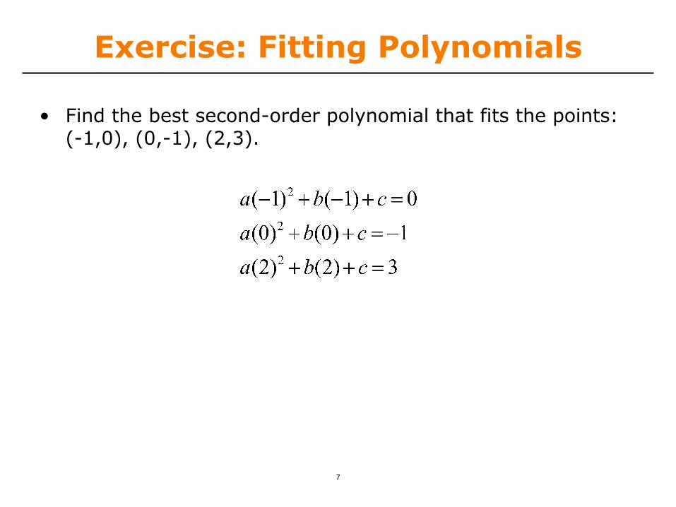
Exercise: Fitting Polynomials

• Find the best second-order polynomial that fits the points:(-1,0), (0,-1), (2,3).

7

Outline

(1) Linear Algebra(2) Polynomials(3) Optimization(4) Differentiation/Integration(5) Differential Equations

8

Polynomials

• Many functions can be well described by a high-orderpolynomial

• MATLAB represents a polynomials by a vector of coefficients➢ if vector P describes a polynomial

ax3+bx2+cx+d

P(1) P(2) P(3) P(4)

• P=[1 0 -2] represents the polynomial x2-2

• P=[2 0 0 0] represents the polynomial 2x3

9

Polynomial Operations

• P is a vector of length N+1 describing an N-th order polynomial• To get the roots of a polynomial

» r=roots(P)➢ r is a vector of length N

• Can also get the polynomial from the roots» P=poly(r)

➢ r is a vector length N

• To evaluate a polynomial at a point» y0=polyval(P,x0)

➢ x0 is a single value; y0 is a single value

• To evaluate a polynomial at many points» y=polyval(P,x)

➢ x is a vector; y is a vector of the same size10

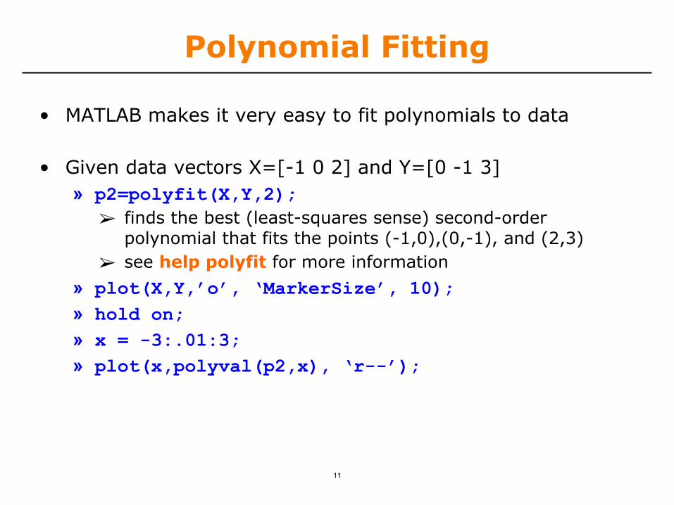
Polynomial Fitting

• MATLAB makes it very easy to fit polynomials to data

• Given data vectors X=[-1 0 2] and Y=[0 -1 3]» p2=polyfit(X,Y,2);➢ finds the best (least-squares sense) second-order

polynomial that fits the points (-1,0),(0,-1), and (2,3)➢ see help polyfit for more information

» plot(X,Y,’o’, ‘MarkerSize’, 10);» hold on;» x = -3:.01:3;» plot(x,polyval(p2,x), ‘r--’);

11

Exercise: Polynomial Fitting

• Evaluate for x=-4:0.1:4.

• Add random noise to these samples. Use randn. Plot thenoisy signal with . markers

• Fit a 2nd degree polynomial to the noisy data

• Plot the fitted polynomial on the same plot, using the samex values and a red line

12

Outline

(1) Linear Algebra(2) Polynomials(3) Optimization(4) Differentiation/Integration(5) Differential Equations

13

Nonlinear Root Finding

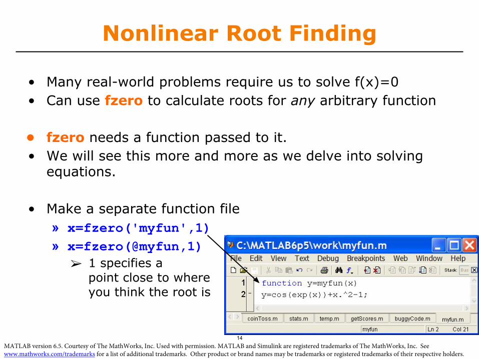
• Many real-world problems require us to solve f(x)=0• Can use fzero to calculate roots for any arbitrary function

• fzero needs a function passed to it.• We will see this more and more as we delve into solving

equations.

• Make a separate function file» x=fzero('myfun',1)» x=fzero(@myfun,1)➢ 1 specifies a

point close to whereyou think the root is

14."5-"#�WFSTJPO������$PVSUFTZ�PG�5IF�.BUI8PSLT �*OD��6TFE�XJUI�QFSNJTTJPO��."5-"#�BOE�4JNVMJOL�BSF�SFHJTUFSFE�USBEFNBSLT�PG�5IF�.BUI8PSLT �*OD���4FF�XXX�NBUIXPSLT�DPN�USBEFNBSLT�GPS�B�MJTU�PG�BEEJUJPOBM�USBEFNBSLT���0UIFS�QSPEVDU�PS�CSBOE�OBNFT�NBZ�CF�USBEFNBSLT�PS�SFHJTUFSFE�USBEFNBSLT�PG�UIFJS�SFTQFDUJWF�IPMEFST�

Minimizing a Function

• fminbnd: minimizing a function over a bounded interval» x=fminbnd('myfun',-1,2);➢ myfun takes a scalar input and returns a scalar output➢ myfun(x) will be the minimum of myfun for -1≤x ≤ 2

• fminsearch: unconstrained interval» x=fminsearch('myfun',.5)➢ finds the local minimum of myfun starting at x=0.5

• Maximize g(x) by minimizing f(x)=-g(x)

• Solutions may be local!

15

Anonymous Functions

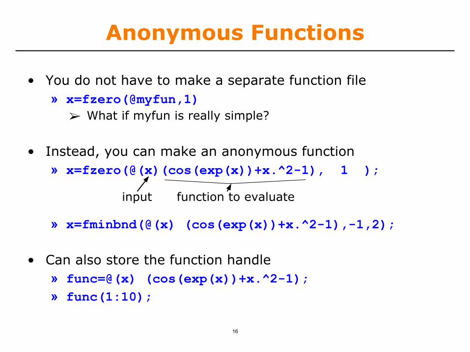
Instead, you can make an anonymous function» x=fzero(@(x)(cos(exp(x))+x.^2-1), 1 );

input function to evaluate

x=fzero(@(x)(cos(exp(x))+x.^2-1), 1 );

• You do not have to make a separate function file» x=fzero(@myfun,1)➢ What if myfun is really simple?

•

» x=fminbnd(@(x) (cos(exp(x))+x.^2-1),-1,2);

• Can also store the function handle» func=@(x) (cos(exp(x))+x.^2-1);» func(1:10);

16

Optimization Toolbox

• If you are familiar with optimization methods, use theoptimization toolbox

• Useful for larger, more structured optimization problems

• Sample functions (see help for more info)» linprog➢ linear programming using interior point methods

» quadprog➢ quadratic programming solver

» fmincon➢ constrained nonlinear optimization

17

Exercise: Min-Finding

• Find the minimum of the functionover the range –π to π. Use fminbnd.

• Plot the function on this range to check that this is theminimum.

18

Digression: Numerical Issues

• Many techniques in this lecture use floating point numbers• This is an approximation!

• Examples:» sin(pi) = ?» sin(2 * pi) = ?» sin(10e16 * pi) = ?➢ Both sin and pi are approximations!

» A = (10e13)*ones(10) + rand(10)➢ A is nearly singular, poorly conditioned (see cond(A))

» inv(A)*A = ?

19

A Word of Caution

• MATLAB knows no fear!

• Give it a function, it optimizes / differentiates / integrates➢ That’s great! It’s so powerful!

• Numerical techniques are powerful but not magic

• Beware of overtrusting the solution!➢ You will get an answer, but it may not be what you want

• Analytical forms may give more intuition➢ Symbolic Math Toolbox

20

Outline

(1) Linear Algebra(2) Polynomials(3) Optimization(4) Differentiation/Integration(5) Differential Equations

21

Numerical Differentiation

• MATLAB can 'differentiate' numerically» x=0:0.01:2*pi;» y=sin(x);» dydx=diff(y)./diff(x);

➢ diff computes the first difference

• Can also operate on matrices» mat=[1 3 5;4 8 6];» dm=diff(mat,1,2)

➢ first difference of mat along the 2nd dimension, dm=[2 2;4 -2]

numerically

mat along themat along the 22nd dimension,dimension, dm=[2dm=[2 2;42;4 -2]-2]

x=0:0.01:2*pi;

dydx=diff(y)./diff(x);first differencefirst differencefirst differencefirst differencefirst differencefirst difference

➢ The opposite of diff is the cumulative sum cumsum

• 2D gradient» [dx,dy]=gradient(mat);

• Higher derivatives / complicated problems: Fit spline (see help)

22

Numerical Integration

• MATLAB contains common integration methods

• Adaptive Simpson's quadrature (input is a function)» q=quad('myFun',0,10)➢ q is the integral of the function myFun from 0 to 10

» q2=quad(@(x) sin(x).*x,0,pi)➢ q2 is the integral of sin(x).*x from 0 to pi

• Trapezoidal rule (input is a vector)» x=0:0.01:pi;» z=trapz(x,sin(x))➢ z is the integral of sin(x) from 0 to pi

» z2=trapz(x,sqrt(exp(x))./x)➢ z2 is the integral of from 0 to pi

23

Outline

(1) Linear Algebra(2) Polynomials(3) Optimization(4) Differentiation/Integration(5) Differential Equations

24

ODE Solvers: Method

• Given a differential equation, the solution can be found byintegration:

➢ Evaluate the derivative at a point and approximate by straight line➢ Errors accumulate!➢ Variable timestep can decrease the number of iterations

25

ODE Solvers: MATLAB

• MATLAB contains implementations of common ODE solvers

• Using the correct ODE solver can save you lots of time andgive more accurate results» ode23➢ Low-order solver. Use when integrating over small intervals

or when accuracy is less important than speed» ode45➢ High order (Runge-Kutta) solver. High accuracy and

reasonable speed. Most commonly used.» ode15s➢ Stiff ODE solver (Gear's algorithm), use when the diff eq's

have time constants that vary by orders of magnitude

26

ODE Solvers: Standard Syntax

To use standard options and variable time step» [t,y]=ode45('myODE',[0,10],[1;0])

ODE integrator: 23, 45, 15s

ODE function Time range

Initial conditions

•

• Inputs:➢ ODE function name (or anonymous function). This function

should take inputs (t,y), and returns dy/dt➢ Time interval: 2-element vector with initial and final time➢ Initial conditions: column vector with an initial condition for

each ODE. This is the first input to the ODE function➢ Make sure all inputs are in the same (variable) order

• Outputs:➢ t contains the time points➢ y contains the corresponding values of the variables

27

ODE Function• The ODE function must return the value of the derivative at

a given time and function value

• Example: chemical reaction 10➢ Two equations

➢ ODE file:– y has [A;B]– dydt has

[dA/dt;dB/dt]

A B50

28

."5-"#�WFSTJPO������$PVSUFTZ�PG�5IF�.BUI8PSLT �*OD��6TFE�XJUI�QFSNJTTJPO��."5-"#�BOE�4JNVMJOL�BSF�SFHJTUFSFE�USBEFNBSLT�PG�5IF�.BUI8PSLT �*OD���4FF�XXX�NBUIXPSLT�DPN�USBEFNBSLT�GPS�B�MJTU�PG�BEEJUJPOBM�USBEFNBSLT���0UIFS�QSPEVDU�PS�CSBOE�OBNFT�NBZ�CF�USBEFNBSLT�PS�SFHJTUFSFE�USBEFNBSLT�PG�UIFJS�SFTQFDUJWF�IPMEFST�

ODE Function: viewing results

• To solve and plot the ODEs on the previous slide:» [t,y]=ode45('chem',[0 0.5],[0 1]);➢ assumes that only chemical B exists initially

» plot(t,y(:,1),'k','LineWidth',1.5);» hold on;» plot(t,y(:,2),'r','LineWidth',1.5);» legend('A','B');» xlabel('Time (s)');» ylabel('Amount of chemical (g)');» title('Chem reaction');

29

ODE Function: viewing results

• The code on the previous slide produces this figure

30

Higher Order Equations• Must make into a system of first-order equations to use

ODE solvers• Nonlinear is OK!• Pendulum example:

."5-"#�WFSTJPO������$PVSUFTZ�PG�5IF�.BUI8PSLT �*OD��6TFE�XJUI�QFSNJTTJPO��."5-"#�BOE�4JNVMJOL�BSF�SFHJTUFSFE�USBEFNBSLT�PG�5IF�.BUI8PSLT �*OD���4FF�XXX�NBUIXPSLT�DPN�USBEFNBSLT�GPS�B�MJTU�PG�BEEJUJPOBM�USBEFNBSLT���0UIFS�QSPEVDU�PS�CSBOE�OBNFT�NBZ�CF�USBEFNBSLT�PS�SFHJTUFSFE�USBEFNBSLT�PG�UIFJS�SFTQFDUJWF�IPMEFST�

31

Plotting the Output

• We can solve for the position and velocity of the pendulum:» [t,x]=ode45('pendulum',[0 10],[0.9*pi 0]);➢ assume pendulum is almost horizontal

» plot(t,x(:,1));» hold on;» plot(t,x(:,2),'r');» legend('Position','Velocity');

Position in terms ofangle (rad)

Velocity (m/s)

32

Plotting the Output

• Or we can plot in the phase plane:» plot(x(:,1),x(:,2));» xlabel('Position');» yLabel('Velocity');

• The phase plane is just a plot of one variable versus theother:

Velocity is greatest when theta=0

Velocity=0 whentheta is the greatest

VelocityVelocityVelocity is greatest whenwhenwhen theta=0

Velocity=0 whentheta is the greatestgreatestgreatest

33

ODE Solvers: Custom Options

• MATLAB's ODE solvers use a variable timestep• Sometimes a fixed timestep is desirable

» [t,y]=ode45('chem',[0:0.001:0.5],[0 1]);➢ Specify timestep by giving a vector of (increasing) times➢ The function value will be returned at the specified points

• You can customize the error tolerances using odeset» options=odeset('RelTol',1e-6,'AbsTol',1e-10);» [t,y]=ode45('chem',[0 0.5],[0 1],options);➢ This guarantees that the error at each step is less than

RelTol times the value at that step, and less than AbsTol➢ Decreasing error tolerance can considerably slow the solver➢ See doc odeset for a list of options you can customize

34

Exercise: ODE

• Use ode45 to solve for on the range t=[0 10], withinitial condition and

• Plot the result.

35

Exercise: ODE

• Use ode45 to solve for on the range t=[0 10], withinitial condition and

• Plot the result.

range t=[0t=[0range t=[0

• Make the following function» function dydt=odefun(t,y)» dydt=-t*y/10;

• Integrate the ODE function and plot the result» [t,y]=ode45(‘odefun’,[0 10],10);

• Alternatively, use an anonymous function» [t,y]=ode45(@(t,y) –t*y/10,[0 10],10);

• Plot the result» plot(t,y);xlabel('Time');ylabel('y(t)');

36

Exercise: ODE

• The integrated function looks like this:

37

MIT OpenCourseWare https://ocw.mit.edu

6.057 Introduction to MATLAB IAP 2019

For information about citing these materials or our Terms of Use, visit: https://ocw.mit.edu/terms.