6.034 Notes: Section 11 - dspace.mit.edu

6.034 Artificial Intelligence by T. Lozano-Perez and L. Kaelbling. Copyright © 2003 by Massachusetts Institute of Technology.

6.034 Notes: Section 11.1

Slide 11.1.1 We have been using this simulated "bankruptcy" data set to illustrate the operation of different learning algorithms that operate on continuous data. Recall that R is supposed to be the ratio of earnings to expenses while L is supposed to be the number of late payments on credit cards over the past year. We will continue using it in this section where we look at a new hypothesis class, the linear separators.

One key observation is that each hypothesis class leads to a distinctive way of defining the decision boundary between the two classes. The decision boundary is where the class prediction changes from one class to another. Let's look at this in more detail.

Slide 11.1.2 We mentioned that the hypothesis for 1-Nearest Neighbor algorithm can be understood in terms of a Voronoi partition of the feature space. The cells illustrated in this figure represent the feature space points that are closest to one of the training points. Any query in that cell will have that training point as its nearest neighbor and the prediction will be the class of that training point. The decision boundary will be the boundry between cells defined by points of different classes, as illustrated by the bold line shown here.

Slide 11.1.3 Similarly, a decision tree also defines a decision boundary in the feature space. Note that although both 1-NN and decision trees agree on all the training points, they disagree on the precise decision boundary and so will classify some query points differently. This is the essential difference between different learning algorithms.


Slide 11.1.4 In this section we will be exploring linear separators which are characterized by a single linear decision boundary in the space. The bankruptcy data can be successfully separated in that manner. But, notice that in contrast to 1-NN and decision trees, there is no guarantee that a single linear separator will successfully classify any set of training data. The linear separator is a very simple hypothesis class, not nearly as powerful as either 1-NN or decision trees. However, as simple as this class is, in general, there will be many possible linear separators to choose from.

Also, note that, once again, this decision boundary disagrees with that drawn by the previous algorithms. So, there will be some data sets where a linear separator is ideally suited to the data. For example, it turns out that if the data points are generated by two Gaussian distributions with different means but the same standard deviation, then the linear separator is optimal.

Slide 11.1.5 A data set that can be succesfully split by a linear separator is called, not surprisingly, linearly separable.

Slide 11.1.6 As we've mentioned, not all data sets are linearly separable. Here's one for example. The classic non-linearly-separable data set is our old nemesis XOR.

It turns out, although it's not obvious, that the higher the dimensionality of the feature space, the more likely that a linear separator exists. This will turn out to be important later on, so let's just file that fact away.

Slide 11.1.7 When faced with a non-linearly-separable data set, we have two options: use a more complex hypothesis class - such as shown here.


Slide 11.1.8 Or, keep the simple linear separator and accept some errors. This is the classic bias/variance tradeoff. Use a more complex hypothesis with greater variance or a simpler hypothesis with greater bias. Which is more appropriate depends on the underlying properties of the data, including the amount of noise. We can use our old friend cross-validation to make the choice if we don't have much understanding of the data.

Slide 11.1.9 So, let's look at the details of linear classifiers. First, we need to understand how to represent a particular hypothesis, that is, the equation of a linear separator. We will be illustrating everything in two dimensions but all the equations hold for an arbitrary anumber of dimensions.

The equation of a linear separator is (surprise!) a linear equation which is determined by n+1 values, the components of an n-dimensional coefficient vector w and a scalar value b. These n+1 values are what will be learned from the data. The x will be some point in the feature space.

We will be using dot product notation for compactness and to highlight the geometric interpretation of this equation (more on this in a minute). Recall that the dot product is simply the sum of the componentwise products of the vector components, as shown here.

Slide 11.1.10 In two dimensions, we can see the interpretation of w and b. The vector w is perpendicular to the linear separator, such a vector is known as the normal vector. Often we say "the vector normal to the surface". The scalar b, which we will call the offset, is proportional to the perpendicular distance from the origin to the linear separator. The constant of proportionality is the negative of the magnitude of the normal vector. We'll examine this in more detail soon.

By the way, the choice of the letter "w" is traditional and meant to suggest "weights", we'll see why when we look at neural nets. The choice of "b" is meant to suggest "bias" - which is the third different connotation of this word in machine learning (the bias of a hypothesis class, bias vs variance, bias of a separator). They are all fundamentally related; they all refer to a difference from a neutral value. To keep the confusion down to a dull roar, we won't call b a bias term but are telling you about this so you won't be surprised if you see it elsewhere.

Slide 11.1.11 Sometimes we will use the following trick to simplify the equations. We'll treat the offset as the 0th component of the weight vector w and we'll augment the data vector x with a 0th component that will always be equal to 1. Then we can write a linear equation as a dot product. When we do this, we will indicate it by using an overbar over the vectors.


Slide 11.1.12 First a word on terminology: the equations we will be writing apply to linear separators in n dimensions. In two dimensions, such a linear separator is refered to as a "line". In three dimensions, it is called a "plane". These are familiar words. What do we call it in higher dimensions? The usual terminology is hyperplane. I know that sounds like some type of fast aircraft, but that's the accepted name.

Let's look at the geometry of a hyperplane a bit more closely. We saw earlier that the offset b in the linear separator equation is proportional to the perpendicular distance from the origin to the linear separator and that the constant of proportionality is the magnitude of the w vector (negated). Basically, we can multiply both sides of the equation by any number without affecting the equality. So, there are an infinite set of equations all of which represent the same separator.

If we divide the equation through by the magnitude of w we end up with the situation shown in the figure. The normal vector is now unit length (denoted by the hat on the w) and the offset b is now equal to the perpendicular distance from the origin (negated).

Slide 11.1.13 It's crucial to understand that the quantity w-hat dot x plus b is the perpendicular distance of point x to the linear separator.

If you recall, the geometric interpretation of a dot product a . b is that it is a number which is the magnitude of a times the magnitude of b times the cosine of the angle between the vectors. If one of the vectors, say a, has unit magnitude then what we have is precisely the magnitude of the projection of the b vector onto the direction defined by a. Thus what dot x is the distance from x to the origin measured perpendicular to the hyperplane.

Look at the right triangle defined by the w-hat and the x vector, both emanating from the origin, we see that the projection of x onto w-hat is the length of the base of the triangle, where x is the hypotenuse and the base angle is theta.

Now, if we subtract out the perpendicular distance to the origin we get the distance of x from the hyperplane (rather than from the origin). Note that when theta is 90 degrees (that is, w and x are perpendicular), the cosine is equal to 0 and the distance is precisely b as we expect.

Slide 11.1.14 This distance measure from the hyperplane is signed. It is zero for points on the hyperplane, it is positive for points in the side of the space towards which the normal vector points, and negative for points on the other side. Notice that if you multiply the normal vector w and the offset b by -1, you get an equation for the same hyperplane but you switch which side of the hyperplane has positive distances.


Slide 11.1.15 We can now exploit the sign of this distance to define a linear classifier, one whose decision boundary is a hyperplane. Instead of using 0 and 1 as the class labels (which was an arbitrary choice anyway) we use the sign of the distance, either +1 or -1 as the labels (that is the values of the yi).

Slide 11.1.16 A variant of the signed distance of a training point to a hyperplane is the margin of the point. This is the actual signed distance for the point times the desired sign of the distance, yi. If they agree, the point is correctly classified, the product is positive; if

they disagree, the classification is in error, then the product is negative.


Slide 11.2.1 So far we've talked about how to represent a linear hypothesis but not how to find one. In this slide is the Perceptron Algorithm, developed by Rosenblatt in the mid 50's. This is not exactly the original form of the algorithm but it is equivalent and it will help us later to see it in this form.

This is a greedy, "mistake driven" algorithm not unlike the boolean learning algorithms we saw earlier. We will be using the extended form of the weight and data points vectors in this algorithm. The extended weight vector is what we are trying to learn.

The first step is to start with an initial value of the weight vector, usually all zeros. The we repeat the inner loop until all the points are correctly classified using the current weight vector. The inner loop is to consider each point. If the point's margin is positive then it is correctly classified and we do nothing. Otherwise, if it is negative or zero, we have a mistake and we want to change the weights so as to increase the margin (so that it ultimately becomes positive).

The trick is how to change the weights. It turns out that using a value proportional to yx is the right thing. We'll see why later. For now, let's convince ourselves that it makes sense.


Slide 11.2.2 Consider the case in which y is positive; the negative case is analogous. If the jth component of x is positive then we will increase the corresponding component of w, note that the resulting effect on the margin is positive. If the jth component of x is negative then we will decrease the corresponding component of w and the resulting effect on the margin is also positive.

Slide 11.2.3 So, each change of w reduces the "error" on a particular point. However, the changes for the different points interfere with each other, that is, different points might change the weights in opposing directions. So, it will not be the case that one pass through the points will produce a correct weight vector. In general, we will have to go around multiple times.

The remarkable fact is that the algorithm is guaranteed to terminate with the weights for a separating hyperplane as long as the data is linearly separable. The proof of this fact is beyond our scope.

Notice that if the data is not separable, then this algorithm is an infinite loop. It turns out that it is a good idea to keep track of the best separator you've seen so far (the one that makes the fewest mistakes) and after you get tired of going around the loop, return that one. This algorithm even has a name (the pocket algorithm - see, it keeps the best answer in it's pocket...).

Slide 11.2.4 This shows a trace of the perceptron algorithm on the bankruptcy data. Here it took 49 iterations through the data (the outer loop) for the algorithm to stop. The hypothesis at the end of each loop is shown here. Recall that the first element of the weight vector is actually the offset. So, the normal vector to the separating hyperplane is [0.94 0.4] and the offset is -2.2 (recall that is proportional to the negative perpendicular distance from origin to the line).

Note that the units in the horizontal and vertical directions in this graph are not equal (the tick marks along the axes indicate unit distances). We did this since the range of the data on each axis is so different.

One usually picks some small "rate" constant to scale the change to w. It turns out that for this algorithm the value of the rate constant does not matter. We have used 0.1 in our examples, but 1 also works well.

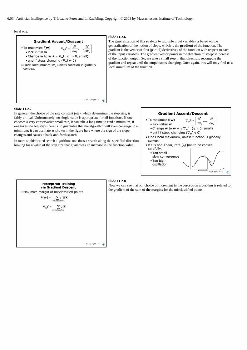
Slide 11.2.5 Let's revisit the issue of why we picked yx to increment w in the Perceptron algorithm. It might have seemed arbitrary but it's actually an instance of a general strategy called gradient ascent for finding the input(s) that maximize a function's output (or gradient descent when we are minimizing).

The strategy in one input dimension is shown here. We guess an initial value of the input. We calculate the slope of the function at that input value and we take a step that is proportional to the slope. Note that the sign of the slope will tell us whether an increase of the input variable will increase or decrease the value of the output. The magnitude of the slope will tell us how fast the function is changing at that input value. The slope is basically a linear approximation of the function which is valid "near" the chosen input value. Since the approximation is only valid locally, we want to take a small step (determined by the rate constant eta) and repeat.

We want to stop when the output change is zero (or very small), this should correspond to a point where the slope is zero, which should be a local extremum of the function. This strategy will not guarantee finding the global maximal value, only a


local one.

Slide 11.2.6 The generalization of this strategy to multiple input variables is based on the generalization of the notion of slope, which is the gradient of the function. The gradient is the vector of first (partial) derivatives of the function with respect to each of the input variables. The gradient vector points in the direction of steepest increase of the function output. So, we take a small step in that direction, recompute the gradient and repeat until the output stops changing. Once again, this will only find us a local minimum of the function.

Slide 11.2.7 In general, the choice of the rate constant (eta), which determines the step size, is fairly critical. Unfortunately, no single value is appropriate for all functions. If one chooses a very conservative small rate, it can take a long time to find a minimum, if one takes too big steps there is no guarantee that the algorithm will even converge to a minimum; it can oscillate as shown in the figure here where the sign of the slope changes and causes a back-and-forth search.

In more sophisticated search algorithms one does a search along the specified direction looking for a value of the step size that guarantees an increase in the function value.

Slide 11.2.8 Now we can see that our choice of increment in the perceptron algorithm is related to the gradient of the sum of the margins for the misclassified points.


Slide 11.2.9 If we actually want to maximize this sum via gradient descent we should sum all the corrections for every misclassified point using a single w vector and then apply that correction to get a new weight vector. We can then repeat the process until convergence. This is normally called an "off-line" algorithm in that it assumes access to all the input points.

What we actually did was a bit different, we modified w based on each point as we went through the inner loop. This is called an on-line algorithm because, in principle, if the points were arriving over a communication link, we would make our update to the weights based on each arrival and we could discard the points after using them, counting on more arriving later.

Another way of thinking about the relationship of these algorithms is that the on-line version is using a (randomized) approximation to the gradient at each point. In fact, the on-line version is sometimes called "stochastic (randomized) gradient ascent" for this reason. In some cases, this randomness is good because it can get us out of shallow local minima.

Slide 11.2.10 Here's another look at the Perceptron algorithm on the bankruptcy data with a different initial starting guess of the weights. You can see the different separator hypotheses that it goes through. Note that it converges to a different set of weights from our previous example. However, recall that one can scale these weights and get the same separator. In fact these numbers are approximately 0.8 of the ones we got before, but only approximately; this is a slightly different separator.

Slide 11.2.11 Recall that the perceptron algorithm starts with an initial guess for the weights and then adds in scaled versions of the misclassified training points to get the final weights. In this particular set of 10 iterations, the points indicated on the left are misclassified some number of times each. For example, the leftmost negative point is misclassified in each iteration except the last one. If we sum up the coordinates of each of these points, scaled by how many times they are misclassified and by the rate constant we get the total change in the weight vector.

Slide 11.2.12 This analysis leads us to a somewhat different view of the perceptron algorithm, usually called the dual form of the algorithm. Call the count of how many times point i is misclassified, alphai. Then, assuming the weight vector is initalized to 0s, we can

write the final weight vector in terms of these counts and the input data (as well as the rate constant).


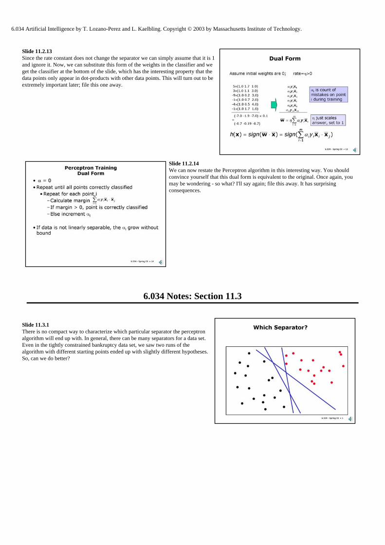
Slide 11.2.13 Since the rate constant does not change the separator we can simply assume that it is 1 and ignore it. Now, we can substitute this form of the weights in the classifier and we get the classifier at the bottom of the slide, which has the interesting property that the data points only appear in dot-products with other data points. This will turn out to be extremely important later; file this one away.

Slide 11.2.14 We can now restate the Perceptron algorithm in this interesting way. You should convince yourself that this dual form is equivalent to the original. Once again, you may be wondering - so what? I'll say again; file this away. It has surprising consequences.


Slide 11.3.1 There is no compact way to characterize which particular separator the perceptron algorithm will end up with. In general, there can be many separators for a data set. Even in the tightly constrained bankruptcy data set, we saw two runs of the algorithm with different starting points ended up with slightly different hypotheses. So, can we do better?


Slide 11.3.2 Yes. One natural choice is to pick the separator that has the maximal margin to its closest points on either side. This is the separator that seems most conservative. Any other separator will be "closer" to one class than to the other. The one shown in this figure, for example, seems like it's closer to the black points on the lower left than to the red ones.

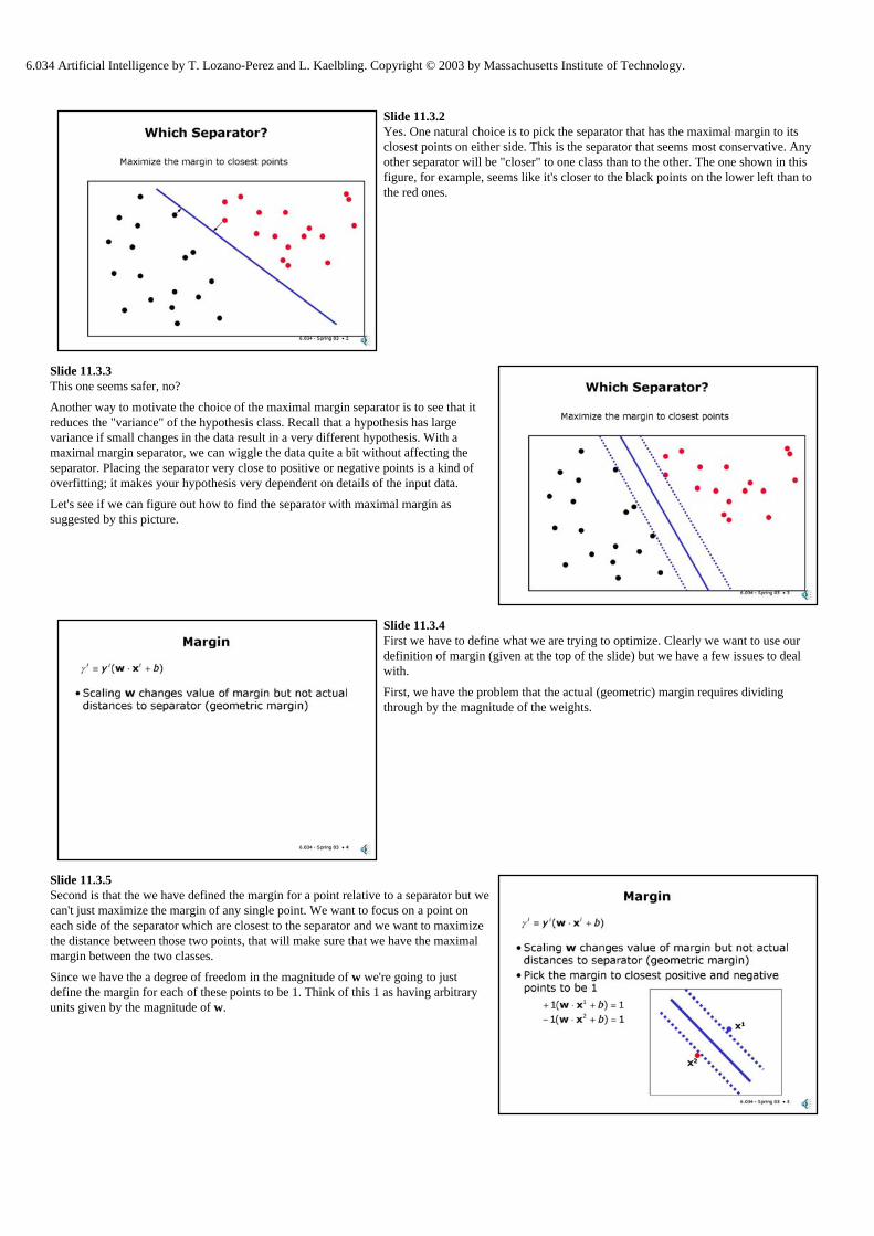
Slide 11.3.3 This one seems safer, no?

Another way to motivate the choice of the maximal margin separator is to see that it reduces the "variance" of the hypothesis class. Recall that a hypothesis has large variance if small changes in the data result in a very different hypothesis. With a maximal margin separator, we can wiggle the data quite a bit without affecting the separator. Placing the separator very close to positive or negative points is a kind of overfitting; it makes your hypothesis very dependent on details of the input data.

Let's see if we can figure out how to find the separator with maximal margin as suggested by this picture.

Slide 11.3.4 First we have to define what we are trying to optimize. Clearly we want to use our definition of margin (given at the top of the slide) but we have a few issues to deal with.

First, we have the problem that the actual (geometric) margin requires dividing through by the magnitude of the weights.

Slide 11.3.5 Second is that the we have defined the margin for a point relative to a separator but we can't just maximize the margin of any single point. We want to focus on a point on each side of the separator which are closest to the separator and we want to maximize the distance between those two points, that will make sure that we have the maximal margin between the two classes.

Since we have the a degree of freedom in the magnitude of w we're going to just define the margin for each of these points to be 1. Think of this 1 as having arbitrary units given by the magnitude of w.


Slide 11.3.6 Having chosen these margins, we can add the two equations to get that the projection of the weight vector on the difference between the two chosen data points has magnitude 2. This is obvious from the setup, but it's nice to see it follows.

Then, we divide through by the magnitude of the weight vector and we have a simple expression for the margin, simply 2 over the magnitude of w.

Slide 11.3.7 So, we want to pick w to maximize the geometric margin, that is, to maximize 2 over the magnitude of w. To maximize this expression, we want to minimize the magnitude of w. If we minimize 1/2 the magnitude squared that is completely equivalent in effect but simpler analytically.

Of course, this is not enough, since we could simply pick w = 0 which would be completely useless.

Slide 11.3.8 So, we want to impose a set of constraints, in particular, we want to pick w so that it classifies points correctly. For each point in the training data we get a linear constraint that says that the margin must be greater or equal to 1. Note that we have chosen the margin for the closest points to be 1 and so the margin for all the points must be at least that.

Slide 11.3.9 So, to summarize, we have defined a constrained optimization problem as shown here. It involves minimizing a quadratic function subject to a set of linear constraints.


Slide 11.3.10 The standard approach to solving this type of problem is to convert it to an unconstrained optimization problem by incorporating the constraints as additional terms in the function to be minimized. Each of the constraints is multiplied by a weighting term alphai. Think of these terms as penalty terms that will penalize values

of w that do not satisfy the constraints.

Slide 11.3.11 To minimize the combined expression we want to minimize the first term (the magnitude of the weight vector squared) but we want to maximize the constraint term since it is negated. Since alphai > 0, making the constraint terms bigger encourages

them to be satisfied (we want the margins to be bigger than 1).

However, the bigger the constraint term, the farther we move from the original minimal value of w. In general we want to minimize this "distortion" of the original problem. We want to introduce just enough distortion to satisfy the constraints. We'll look at this in more detail momentarily.

Slide 11.3.12 This method we have begun to outline here is called the Method of Lagrange Multipliers and the alphai are the individual Lagrange multipliers.

Slide 11.3.13 Let's look at this more closely by looking at a very simple example. This problem is basically like our problem but for a single weight w and no offset term.


Slide 11.3.14 The first step is to incorporate the constraint and define a new function L which is a function of w, with alpha as an additional parameter. This function is the Lagrangian.

Slide 11.3.15 We can plot L(w) as a function of w for several values of alpha. Note that as expected, as alpha grows the value of w for which L(w) is minimal gets farther and farther from the original value of 0. Note that for alpha=1, the value of w for which L(w) is minimal (that is, w=1) satisfies the constraint with minimal distortion. Values of alpha less than 1 don't satisfy the constraint and larger values of alpha distort the original minimum more.

If you look at the figure, you can see that the value of L(w) at the minimum is also greatest for alpha=1. Is this a coincidence? We'll see that it isn't.

Slide 11.3.16 To minimize the Lagrangian L(w), we need to set dL/dw to zero. This is extremely easy and it gives us a simple linear equation which we solve to get that the optimal value of w (denoted w*) is simply alpha times x.

Setting the derivative to zero gives us a "critical point" which could be a minimum, a maximum or simply an inflection point. Looking at the second derivative with respect to w, we see that it is 1. A positive second derivative tells us we have a minimum with respect to w.

Slide 11.3.17 We can substitute this expression for w* back into L(w) to get the value of L at its minimum for any value of alpha (recall that the x are constants from the training data). We looked at these minima for three values of alpha a few slides back. Now we have an expression that gives us the minimal values for all values of alpha. This is called the Lagrangian dual (for reasons beyond the scope of the course).


Slide 11.3.18 Based on our earlier observations, it seems as we should be interested in the value of alpha that maximizes L(alpha). We can find the maximum of L(alpha) by setting dL/dalpha to 0. This gives us a simple equation for the optimal alpha - 1 - 1/2 alpha x2

= 0. We can also re-write this in terms of our optimal w, as 1 - w*x = 0.

We can see that this critical point is a maximum by checking that the second derivative with respect to alpha is -x2, which is always negative. This is sufficient to identify this critical point as a maximum.

Slide 11.3.19 Interestingly, this maximum of alpha corresponds precisely to the value of w where the constraint is satisfied with equality and where we distort the original minimum the least.

The fact that the maximum with respect to alpha of the Lagrangian dual has this property is a non-trivial result, well beyond our scope. This idea even has a name - the Wolfe Dual.

Slide 11.3.20 Recall that alpha is constrained to be greater than or equal to 0. What happens if we get the maximum of L(alpha) for negative alpha? Observe that for any value of alpha greater than the optimal alpha the inequality constraint will also be satisfied (with margins greater than 1). So, we can choose alpha to be 0 and cause no distortion in our original minimum of L(w). Basically, we have found that the constraint is not binding at the optimal value of w.

Alternatively, if the alpha at the maximum is positive then this corresponds to satisfying the constraint at equality (the margin is exactly 1).

This is basically everything we need to know about maximizing margins. Let's summarize what we did. Let's review the steps we followed with this simple example because they're exactly the steps that we will follow with the more general case.

1. We started trying to minimize the magnitude of the weight vector subject to a set of constraints on the size of the margin for each of the points in the data set. 2. We defined the Lagrangian by incorporating all the constraints, via Lagrange

multipliers, into a single function of w to be optimized. 3. We found the minimum of the Lagrangian with respect to w and obtained a simple linear relationship between the weight vector and

alpha. 4. We substituted this relationship into the original Lagrangian and obtained the dual Lagrangian L(alpha), which gives us the minimum of

L(w) as a function of alpha. 5. We then maximize the dual Lagrangian to obtain the optimal value of the Lagrange multiplier (alpha). 6. We can use the relationship between w and alpha to find the optimal w.

We will now go through this same process for the general case of multiple weights and multiple constraints.



Slide 11.4.1 This is our original Lagrangian we set up to optimize the margin for a linear separator. Note that we need to solve for the weights w and the offset b. That is, we are solving for n+1 variables, where n is the dimensionality of the data.

We also have m Lagrange multipliers in the formulation, each associated with a linear constraint obtained from a data point.

Slide 11.4.2 Now, we find the minima of L with respect to all n+1 variables by setting all the first derivatives of the Lagrangian to zero. When we show a derivative of a function with respect to a vector this refers to the vector of derivatives with respect to each of the components of the vector.

Slide 11.4.3 Using the derivative rules shown at the bottom of the slide, we can get expressions for the derivatives of L.


Slide 11.4.4 Note that the derivative with respect to alpha is very similar to what we saw in our simple example and leads to a value for the optimal w in terms of alpha, just as before. Now we also have a derivative with respect to the offset b which gives us a linear constraint on all the alpha's.

Slide 11.4.5 We can now substitute the expression for w in terms of alpha and use the constraint on the alphas to derive an expression for the dual Lagrangian which involves only alphas and the input data.

In particular, note that the data point feature vectors don't show up except in dot products (remember, the value of a dot product is a scalar). So, someone can give us an m x m matrix of dot products of the feature vectors and we can solve for the optimal alphas; they don't actually need to tell us what the feature vectors actually are. This will prove important later.

Slide 11.4.6 Now we proceed to maximize the dual Lagrangian. Note that there are m alphas that we solve for. We started with n+1 variables in the original Lagrangian and now we have m variables in the dual Lagrangian. For the low-dimensional examples we have been dealing with this seems like a horrible tradeoff. We will see in the next lecture that this can be a very good tradeoff in some circumstances.

We have two constraints, but they are much simpler. One constraint is simply that the alphas be non-negative - this is required because our original constraints were >= inequalities. The linear constraint on the alphas comes from the setting to zero the derivative of the Lagrangian with respect to the offset b.

This problem is not trivial to solve in general; we'll talk more about this later. For now, let us assume that we can solve it and get the optimal values of alphas.

Slide 11.4.7 The same situation we described in the simple example holds. Most of the alphas will be zero, corresponding to data points that do not provide binding constraints on the choice of the weights. A few of the data points will have their alphas be nonzero; they will all satisfy their constraints with equality. These are called support vectors and they are the ones used to define the maximum margin separator. You could remove all the other data points and still get the same separator.


Slide 11.4.8 Given the optimal alphas, we can compute the weights. This is just like we did in the dual perceptron.

Slide 11.4.9 We can use the fact that at the support vectors the constraints hold with equality to solve for the value of the offset b. Each such constraint can be used to solve for this scalar. In the absence of numerical error, the value one gets from all the binding constraints should be the same. In practice, due to numerical inaccuracies, it is better to use the average of the values obtained from each of the binding constraints.

Slide 11.4.10 We have not discussed actual algorithms for finding the maxima of the dual Lagrangian. It turns out that the optimization problem we defined is a relatively simple form of quadratic programming problem which are known to (a) have a unique maximum and (b) can be found using existing algorithms. A number of variations on these algorithms exist but they are (again) beyond our scope.

Slide 11.4.11 Interestingly, we can approximate the answer using gradient ascent. The only troublesome part is the presence of the linear constraint on the alphas, which means that we can't change the alphas independently. If we assume that the offset it zero, then we can ignore this constraint and solve for the alphas and then the weights. This gives us a hyperplane that goes through the origin. In high dimensional problems this is not much of a restrictions but it is a substantial limitation in the low-dimensional examples we have been looking at.

You may wonder why we don't simply incorporate the offset into the weight vector as we've done before. The problem is that then we would be changing the magnitude of w and thereby changing the margin. In many cases, this may be ok but it's not the optimal answer in general.


Slide 11.4.12 The resulting gradient descent method to find the Max Margin classifier is called the "Adatron". To make this work reliably one has to fiddle quite a bit with the learning rate, usually one picks a different learning rate for each point! But the idea is simple.

Slide 11.4.13 Here's the result of running a quadratic programming algorithm to find the maximal margin separator for the bankruptcy example. Note that only four points have non-zero alpha's. They are the closest points to the line and are the ones that actually define the line.

Slide 11.4.14 What happens when the data are not perfectly separable by a linear separator? This is in fact, the usual case.

It turns out that there's a relatively simple strategy that's effective. We pick a parameter C (which will need to be chosen for each problem) which will be the limit on the maximum value of any of the alpha's. This means that no point can ever contribute more than C to the construction of the weights. So, the influence of "outlier" points is limited.

Recall the intuition from the dual perceptron that the magnitude of alpha is related to how many times a point has been misclassified. In general, the magnitude of the alpha will reflect how much we allow any point to distort the values of the weights from their optimal values (maximal margin). We are capping this amount and saying that we are willing to live with some misclassifications.

The lower C is, the more willing we are to accept misclassifications.

Slide 11.4.15 This simple example shows how changing C causes the geometric margin to change. For low values of C the margin between positives and negatives is reduced as the algorithm tries to "capture" the wayward point off on the right. For high values of C, the separator is closer to where it would be if the "outlier" were not there.


Slide 11.4.16 The linear separator is very simple hypothesis class but it can perform very well on appropriate data sets. On the Wisconsin Breast Cancer data, the maximal margin classifier does as well or better as any of the other classifiers we have seen on held-out data. Note that only 37 of the 512 training points are support vectors.

Of course, it is easy to find or construct data sets where performance will be poor. In the next Chapter, we will see several extensions to the ideas presented here that will allow us to develop methods that are much more general and powerful.

6.034 Notes: Section 11 - dspace.mit.edu

Documents

Transcript of 6.034 Notes: Section 11 - dspace.mit.edu