60-539: Emerging non-traditional database systems (Data...

60-539: Emerging non-traditional database systems (Data Warehousing and Mining):

60-539 Dr. C.I. Ezeife @c 2018 1

sdb1

sdb2

sdb3

Dr. C.I. EzeifeSchool of Computer Science,University of Windsor, Canada.Email: [email protected]

warehouse

PART I (DATABASE MANAGEMENT

SYSTEM OVERVIEW)

DBMS (PART 1) OVERVIEW

Components of a DBMS

DBMS Data model

Data Definition and Manipulation Language

File Organization Techniques

Query Optimization and Evaluation Facility

Database Design and Tuning

Transaction Processing

Concurrency Control

Database Security and Integrity Issues

60-539 Dr. C.I. Ezeife © 2018 2

DBMS OVERVIEW(What are?)

What is a database? : It is a collection of data, typically describing the activities of one or more related organizations, e.g., a University, an airline reservation or a banking database.

What is a DBMS?: A DBMS is a set of software for creating, querying, managing and keeping databases. Examples of DBMS’s are DB2, Informix, Sybase, Oracle, MYSQL, Microsoft Access (relational).

Alternative to Databases: Storing all data for university, airline and banking information in separate files and writing separate program for each data file.

What is a Data Warehouse?:A subject-oriented, historical, non-volatile database integrating a number of data sources.

What is Data Mining?:Is data analysis for finding interesting trends or patterns in large dataset to guide decisions about future activities.

60-539 Dr. C.I. Ezeife © 2018 3

DBMS OVERVIEW(Evolution of

Information Technology)

1960s and earlier: Primitive file processing: data are collected in files

and manipulated with programs in Cobol and other languages.

Disadv.: any change in storage structure of data requires changing the

program (i.e., no logical or physical data independence). Data and

programs are also replicated as there is no central management.

1970s – early 1980s: DBMSs used, which is a set of software for

creating, querying, managing and keeping large collections of data.

Hierarchical and network dbms came before relational (called

traditional because of its wide use and success in business).

• Advs of DBMS: (1) Logical data independence:Users can be

shielded from changes in the logical structure of data (eg, adding

fields or tables) or in the choice of relations to be stored through

external schema (eg, views).

60-539 Dr. C.I. Ezeife © 2018 4

DBMS OVERVIEW(Evolution of

Information Technology)

• (2) Physical data independence: The conceptual schema hides details regarding how data are actually stored on disk so that change in physical data storage does not affect use of the conceptual schema.

• (3)Efficient data access, data integrity and security, data administration, concurrent access and crash recovery, reduced application development time.

1980’s to present: Advanced (Non-Traditional) DBMSs: These include object-oriented database systems, object-relational databases, deductive databases, spatial, temporal, multimedia, active, scientific databases and knowledge bases.

Late 1980s to present: Other Advanced DBMSs like Data Warehousing and Mining.

1990’s to present: Web-based DBMS, XML-based DBMS and web mining.

60-539 Dr. C.I. Ezeife © 2018 5

DBMS OVERVIEW(3 Levels of Data

Abstraction)

The database consists of a schema at each of the 3 levels:

(1)External level – allows for customization of data access in terms of

individual or group of users. Each external schema consists of a

collection of one or more views. A view is computed from stored

relations.

(2)Conceptual level – describes the stored data in terms of the data

model of the DBMS (e.g., relation in relational DBMS).

(3) Physical level - specifies additional storage details by summarizing

how the relations in the conceptual schema are stored on disk (e.g.,

what file organizations like indexes to speed up operations).

60-539 Dr. C.I. Ezeife © 2018 6


A DBMS has the following basic components

• 1. A specific data model: the data structure for logically

representing data by the DBMS (e.g., relational, object-oriented,

hierarchical etc.).

• 2. A Data definition and data manipulation language for creating

files in the database and querying the database (e.g., SQL, QBE).

• 3. File Organization techniques for storing data physically on disk

efficiently (e.g., B+-tree indexing or ISAM indexing).

• 4. Query Optimization and Evaluation facility: helps to generate

the best query plan for executing a query efficiently.

60-539 Dr. C.I. Ezeife © 2018 7


• 5. Database Design and Tuning: Allows schema design

at the conceptual level (e.g., normalization,

fragmentation of data and performance tuning).

• 6. Transaction Processing

– Concurrency Control and recovery: Allowing more

than one user access data concurrently and

maintaining a consistent and correct data even after

hardware or software failure.

– Database Security and Integrity Issues: Protecting

data from inconsistent changes made by different

concurrent users.

60-539 Dr. C.I. Ezeife © 2018 8

Other Non-Traditional DBMSs

To handle requirements of new complex applications, new database

systems have emerged and include:

1. Object-Oriented Databases: database entities are objects; and codes

relating to an object are encapsulated in the object. Each object has a

set of attribute values and a set of methods for communicating with the

object. Each object belongs to a class defined in an inheritance

hierarchy in the db schema. A class may have subclasses and

superclasses. OODB can be used for computer aided engineering

design data like for buildings, cars, airplanes.

2. Object-Relational Databases: Build databases that capture OO

features using extended relational system for handling complex object

class hierarchies (e.g, use of nested relations)

60-539 Dr. C.I. Ezeife © 2018 9


3.Spatial Databases: Contain spatial-related information like

geographic (maps) databases, medical and satellite image databases.

4. Temporal Databases and Time-Series Databases:store time-related

data: Temporal db contains time-related attrs with different semantics

(e.g., jacket in fall, winter). A time-series db stores sequences of values

that change with time.

5. Text databases and Multimedia Databases:contain word descriptions

of objects. Text db may be highly unstructured, or semi-structured

(e.g., HTML/XML pages), or structured(e.g., library dbs).

60-539 Dr. C.I. Ezeife © 2018 10


6. Heterogeneous and Legacy Databases: A legacy db is a group of

heterogeneous dbs that combines different kinds of data systems like

OO, relational, files, html etc. via a network.

7. World Wide Web and NOSQL dbs: distributed information services

on the web such as Google, Yahoo, Alibaba, Mapquest that provide

interactive access through linking of web objects in applications

providing access to data through NOSQL (not only SQL) means.

8. Data Warehouses: are integrated, subject-oriented, time-variant,

non-volatile, summarized collection of data from a number of possibly

heterogeneous data sources unified under one schema.

60-539 Dr. C.I. Ezeife © 2018 11

1. DBMS Data model

Data model provides the data structure that the database is

stored in at the conceptual level, and the operations

allowed on this data structure.

Some existing DBMS data models are relational, entity-

relationship model, object-oriented and hierarchical data

model.

Schema in the relational model is used to describe the data

in the database.

60-539 Dr. C.I. Ezeife © 2018 12

1. DBMS Data model

60-539 Dr. C.I. Ezeife © 2018 13

• Example of a relational instance of the table student is given above.

Example of integrity constraint that can be defined on this table is “Every

student has a unique id”.

• Concepts associated with the relational db include:relation schema and

instance, db schema, primary key, super key, candidate key, foreign key,

cardinality and degree of a relation, integrity constraints.

student Studid Name gpa

53666 Jones S 3.4

53688 Smith M 3.2

53650 Smith J 3.8

53831 Madayan A 1.8

53832 Guldin 2.0

1. DBMS Data model

Data in DBMS are described in 3 levels of abstraction

namely:

• External schema (representing how different users view

the data). E.g., view for students with gpa > 3.2

• Conceptual Schema (logical schema) - data described in

terms of data model (e.g.)

– student (stuid:string, name:string, gpa:real)

– faculty (fid:string, fname:string, salary:real)

– courses (cid:string, cname:string, credits:integer)

– Rooms (rno: integer, address:string, capacity:integer)

– Enrolled (sid:string, cid:string, grade: string)

60-539 Dr. C.I. Ezeife © 2018 14

1. DBMS Data model

– Teaches (fid:string, cid:string)

– Meets_In (cid:string, rno:integer, time:string)

• Physical Schema: describes how data are actually

stored on disks and tapes including indexes. Example

physical design are:

– store all relations as unsorted files of records

– create indexes on the first column of student, faculty and course

relations, the salary column of faculty and capacity column of rooms.

60-539 Dr. C.I. Ezeife © 2018 15

2. Data Definition, Manipulation, Control Languages (DDL, DML, DCL)

Example of a DDL, DML and DCL language is with structured query language (SQL).

Basic DDL, DML, DCL operations for SQL (structured query lang):

A: Data Definition Language (DDL) of SQL allows us create new database structures like tables, views and indexes and to modify existing tables. The SQL DDL commands are:

• 1. Create tables [Create Table …]

• 2. Destroy tables [Drop Table …]

• 3. Alter tables [Alter Table ….]

• 4. Truncate tables [Truncate Table Student]

• 5. Rename tables [Rename oldname To newname]

60-539 Dr. C.I. Ezeife © 2018 16


Data Manipulation Language (DML) commands allow us to query,

insert, update or delete data and include the following:

• 6. Insert Data into Tables [Insert Into ….]

• 7. Delete Data from Tables [Delete from …]

• 8. Update Data in Tables [Update …. ]

• 9. Merge tables [Merge Into tablename …]

• 10. Query Tables [Select … from … where … ]

• 11. Find the structure of DB, relation, view, index, etc.[querying

catalogue with select * from tab; select * from cat; Desc Table;

etc.]

60-539 Dr. C.I. Ezeife © 2018 17


C. Data Control Language (DCL) of SQL is used to control

access to the stored data and include the following

commands:

12. Grant [Grant All to user_music]

13. Revoke [Revoke update on Student from user_music]

The document in file SQL_some handed out in class

contains summary and example use of these SQL

commands.

60-539 Dr. C.I. Ezeife © 2018 18

2 Transaction Control Language Commands

SQL commands used for saving or commiting database updates, undoing them or creating break points in transactions for effecting such undoing of tasks are transaction control commands and these include:

1. COMMIT 2. ROLLBACK 3. SAVEPOINT

The session issuing the DML command can always see the changes, but other sessions can only see the changes after you commit. DDL and DCL commands implicitly issue a COMMIT to the database. The Rollback command undoes any DML statements back to the last COMMIT command issued. The SAVEPOINT allows us to save the result of DML transactions temporarily up to a particular marked SAVEPOINT.

60-539 Dr. C.I. Ezeife © 2018 19

2. Data Definition and Manipulation

Languages (DDL & DML)

In order to create and query database tables, user needs to connect to SQL interpreter called Sqlplus as follows:

1. From Unix account, type:

>Sqlplus

>username

>password

2. To quit sqlplus, type:

> exit

3. To load and run a .sql file, type:

> @filename

4. To execute a SQL command like “Create Table …”, type:

> Create Table student(stuid VARCHAR(20), ….;

60-539 Dr. C.I. Ezeife © 2018 20



• DDL is used to create and delete tables and views, and to modify table structures. E.g. of an SQL instruction for creating the table student is:

CREATE TABLE student (stuidVARCHAR2(20),

name VARCHAR2 (20),gpa NUMBER(5,2),CONSTRAINT student_pk PRIMARY

KEY (stuid));

60-539 Dr. C.I. Ezeife © 2018 21



• To destroy a table or view, e.g., student, use:

– DROP TABLE student RESTRICT;

– or

– DROP TABLE student CASCADE CONSTRAINTS;

• The RESTRICT keyword prevents the table from being destroyed if some integrity constraints are defined on it. The CASCADE keyword destroys both the parent table student and any constraints on a child table like foreign key constraint from Enroll that references the dropped table student .

• To modify table structure, use:

– ALTER TABLE student ADD COLUMN major CHAR (20);

60-539 Dr. C.I. Ezeife © 2018 22



The DML subset of SQL is used to pose queries and to

insert, delete and modify rows of tables.

For example, to query the student table in order to print

the ids, names and gpas of all students with gpa > 3.2, we

use:

• SELECT s.stuid, s.name, s.gpa

FROM student s

WHERE s.gpa > 3.2;

The basic form of an SQL query is as follows:

60-539 Dr. C.I. Ezeife © 2018 23



• SELECT [DISTINCT] select-list

FROM from-list

WHERE qualification;

from-list is a list of table names possibly followed by a

range variable.

Select-list is a list of (expressions) column names of tables

from the from-list.

The qualification is a Boolean combination in the form

expression op expression with possible connectives (AND,

OR, NOT)

60-539 Dr. C.I. Ezeife © 2018 24

2. Data Definition and Manipulation Languages

(DDL & DML)

60-539 Dr. C.I. Ezeife © 2018 25

Sid sname rating age

22 dustin 7 45.0

31 lubber 8 55.5

58 rusty 10 35.0

Sid sname rating age

28 yuppy 9 35.0

31 lubber 8 55.0

44 guppy 5 35.0

58 rusty 10 35.0

Sailors: instance S2

Sid bid day

22 101 10/10/2011

58 103 11/12/2011

Reserves: instance R1

Sailors reserve boats

world. Sailors instance S1



DISTINCT keyword is optional and eliminates duplicate

tuples.

E.g., find the names of sailors who have reserved boat

number 103.

• Select S.sname

from sailors S, Reserves R

where S.sid = R.sid

And R.bid = 103;

60-539 Dr. C.I. Ezeife © 2018 26



Aggregate Operators

SQL supports a more general version of column list

Each item in a column list can be of the form expression

AS column-name, where expression is any arithmetic or

string expression over column names and constants.

A column-list can also contain aggregates (sum, count, avg,

min, max).

It supports pattern matching through the LIKE operator,

along with the use of wild-card symbols

60-539 Dr. C.I. Ezeife © 2018 27



% (zero or more characters) and - (exactly one arbitrary

character).

E.g., Find the ages of sailors whose name begins and ends

with B and has at least three characters.

• SELECT S.age

from sailors

where s.name LIKE ‘B - %B’;

SQL supports the set operations unions, intersect and

difference under names UNION, INTERSECT, and

EXCEPT.

60-539 Dr. C.I. Ezeife © 2018 28



Nested Queries

A nested query is a query that has another query

embedded within it. The embedded query is called

subquery.

E.g., Find the names of sailors who have reserved boat

number 103.

• Select s.same

from sailors S

where s.sid IN (Select R.sid

from Reserves R

where R.bid = 103);

60-539 Dr. C.I. Ezeife © 2018 29



Can also be expressed as:

• Select S.sname

from sailors S

where Exists (Select *

from Reserves R

where R.bid = 103

And S.sid = R.sid);

The latter version is a correlated nested query

Other set comparison operators are UNIQUE, ANY, ALL.

IN and NOT IN are equivalent to =ANY and <>ALL respectively.

60-539 Dr. C.I. Ezeife © 2018 30



The Group By and Having Clauses

Example, find the age of the youngest adult sailor for each

rating level with at least 2 such sailors.

• Select S.rating, MIN(S.age) AS minage

from Sailor S

where S.age >= 18

Group by S.rating

Having Count(*) > 1;

60-539 Dr. C.I. Ezeife © 2018 31



General SQL form is

• Select [Distinct] select-list

from from-list

where qualification

Group by grouping-list

Having group-qualification;

Result is

60-539 Dr. C.I. Ezeife © 2018 32

Rating minage

3 25.5

7 35.0

8 25.5



• Null Values• A new sailor, Bob, may not have a rating assigned,

leaving the data value for this column unknown.• Some columns may be inapplicable to some

sailors, e.g., column maiden-name is inapplicable to men and single women sailors.

• SQL provides a column value for these kinds of situations.

• SQL provides a comparison operator to test if a column value is null (IS NULL) and (IS NOT NULL).

60-539 Dr. C.I. Ezeife © 2018 33



NOT (unknown) is unknown

false OR unknown is unknown

true OR unknown is true

true AND unknown is unknown

unknown AND unknown is unknown

The arithmetic operations +, -, * and / all return null if one of their

arguments is null

COUNT(*) counts null values like other values while other aggregate

functions treat it as no value.

Null values can be disallowed by specifying NOT NULL as part of the

field definition. E.g., sname CHAR(20) NOT NULL.

60-539 Dr. C.I. Ezeife © 2018 34


Languages (DDL & DML- Embedded)

• Note: Slides 35 to 44 are to inspire additional reading if needed.

• Building db applications with nice graphical user interface would require facilities provided by general purpose langs in addition to SQL. The use of SQL commands within a host langprogram is called embedded SQL.

• In embedded SQL, SQL statements are used wherever a stmtin the host lang is allowed and SQL stmts are clearly marked. Eg., in C (e.g., Oracle Pro*C), SQL stmts must be prefixed by EXEC SQL

• Any host lang variable for passing arguments into an SQL command must be declared in SQL. Such host lang variables must be prefixed by ( : ) in SQL stmts and be declared between the commands EXEC SQL BEGIN DECLARE SECTION and EXEC SQL END DECLARE SECTION.

60-539 Dr. C.I. Ezeife © 2018 35



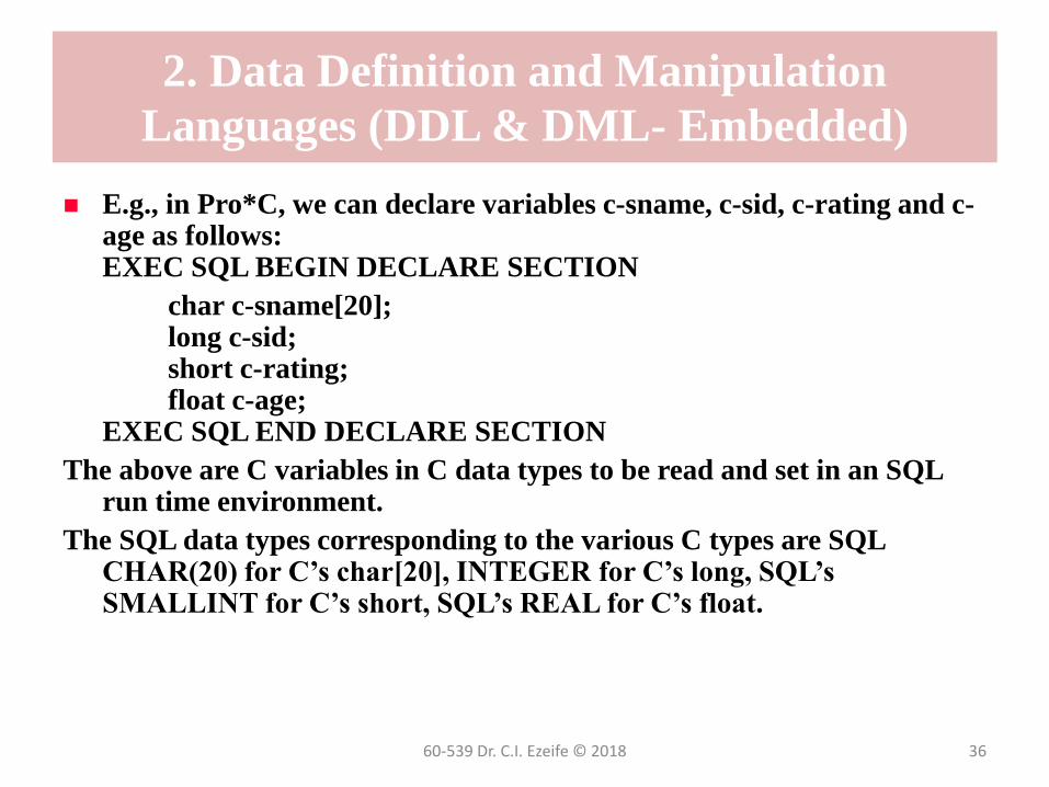
E.g., in Pro*C, we can declare variables c-sname, c-sid, c-rating and c-age as follows:EXEC SQL BEGIN DECLARE SECTION

char c-sname[20];long c-sid;short c-rating;float c-age;

EXEC SQL END DECLARE SECTION

The above are C variables in C data types to be read and set in an SQL run time environment.

The SQL data types corresponding to the various C types are SQL CHAR(20) for C’s char[20], INTEGER for C’s long, SQL’s SMALLINT for C’s short, SQL’s REAL for C’s float.

60-539 Dr. C.I. Ezeife © 2018 36



One of the two special variables (SQLCODE, SQLSTATE) for reporting errors

must be declared in an embedded SQL program.

While SQLCODE (of type long) simply returns a negative number when an

error occurs, SQLSTATE (of type char[6]) associates a predefined value with

some error conditions.

SQLSTATE variable should be checked for errors and exceptions after each

embedded SQL stmt using the WHENEVER command:

EXEC SQL WHENEVER [SQLERROR | NOT FOUND] [CONTINUE |

GOTO stmt]

E.g., SQLSTATE is set to the value of 02000 denoting NO DATA.

While SQL operates on sets of records, langs like C do not support sets of

records.

Thus, cursors are used to retrieve rows one at a time from a relation.

60-539 Dr. C.I. Ezeife © 2018 37



A cursor can be declared on any relation or on any SQL query. Once a

cursor is declared, we can (1) open it (to position the cursor just before

the first row); (2) fetch the next row; (3) move the cursor to the next

row, row after the next, first row, previous row, etc. by specifying

additional parameters to the FETCH commands; (4) close the cursor.

INSERT, DELETE and UPDATE stmts typically require no cursor.

SELECT needs cursor for a number of rows, but SELECT for just one

row does not need a cursor. E.g.,

EXEC SQL SELECT s.sname, s.age

INTO :c-sname, :c-age

FROM Sailors S

WHERE S.sid = :c-sid;

60-539 Dr. C.I. Ezeife © 2018 38


Languages (DDL & DML- JDBC/ODBC)

ODBC (open database connectivity) and JDBC (Java database

connectivity) also allow integration of SQL with a general purpose

programming lang.

ODBC and JDBC connect to databases through application

programming interface (API).

ODBC and JDBC connectivity provide more portable access to

different database management systems than embedded SQL.

With ODBC and JDBC, all interactions with a specific DBMS occurs

through a DBMS specific driver.

The driver is responsible for translating ODBC or JDBC calls into

DBMS-specific calls.

Available drivers are registered with a driver manager.

60-539 Dr. C.I. Ezeife © 2018 39


Languages (DDL & DML- JDBC/ODBC)

How JDBC works: (1) A database application (e.g., a java program for inserting rows of records into an Oracle database), selects each data source (i.e dbms) it wants to connect to (can be more than 1); (2) Application then loads and connects to each selected data source, which are now open connections. While a connection is open, transactions are executed by submitting SQL stmts, retrieving results of SQL queries, processing errors and finally committing or rolling back; (3) Application disconnects from the data source to terminate the interaction.

JDBC is a collection of Java classes and interfaces for enabling database access from programs written in Java lang.

The JDBC classes and interfaces are part of the java.sql package. Thus, all Java database applications should include at beginning

import java.sql.*

60-539 Dr. C.I. Ezeife © 2018 40


(DDL & DML- Stored Procedures like PL/SQL)

A stored procedure is a program executed through a single SQL stmtlocally executed and completed within the process space of the database server.

Once a stored procedure is registered with the db server, different users can re-use it.

All major db systems provide ways for users to write stored procedures in a simple general purpose lang close to SQL – e.g., Oracle PL/SQL.

A stored procedure is declared as:CREATE PROCEDURE name(parameter1, …., parameterN)

local variable declarationsprocedure code;

If the first CREATE line returns a single sqlDataType, it becomes a stored function.

60-539 Dr. C.I. Ezeife © 2018 41



Each parameter is a triple containing mode (IN, OUT or INOUT), parameter name, and parameter SQL datatype.

IN indicates an input parameter to the procedure, OUT indicates an output parameter for holding result from the procedure, while INOUT indicates a parameter that is passed to the procedure and which can also be changed to return results. E.g. function:CREATE PROCEDURE RateCustomer (IN custId INTEGER,

IN year INTEGER) RETURNS INTEGERDECLARE rating INTEGER;DECLARE numOrders INTEGER;SET numOrders=(SELECT COUNT(*) FROM Orders O

where O.cid=custId);IF (numOrders > 10) THEN rating = 2;ELSIF (numOrders >5) THEN rating = 1;ELSE rating = 0;END IF;RETURN rating;

60-539 Dr. C.I. Ezeife © 2018 42



Local variables are declared using DECLARE stmt and values are

assigned using the SET stmt, but returned with the RETURN stmt

Branch instruction is of the form:

IF (condition) THEN statement;

ELSIF statements;

END IF;

Loops are of the form:

LOOP

statements;

END LOOP

A procedure stmt can be an SQL query, a SET stmt, a branch or loop

stmt, a CALL stmt or a RETURN stmt.

60-539 Dr. C.I. Ezeife © 2018 43



SQL queries can be used as expressions in branches and stmts.

Cursor stmts can be used without EXEC SQL prefix and no colon (:)

before variables in these stmts.

A stored procedure may have no parameter as in:

CREATE PROCEDURE ShowNumberOfOrder

SELECT C.cid, C.cname, Count(*) FROM Customers C,

Orders O, WHERE C.cid=O.cid GROUP BY C.cid, C.cname;

Stored procedures can be called in interactive SQL with the CALL

stmt using the format:

CALL storeProcedureName(arg1, arg2, .., argN);

Stored procedures do not have to be written in SQL as they can be

written in any host lang like JAVA.

60-539 Dr. C.I. Ezeife © 2018 44

2. Relational Algebra and Calculus

Two formal query langs. associated with the relational

model are relational algebra and calculus.

A relational algebra operator accepts one or 2 relation

instances as arguments and returns a relation instance as

output

Basic algebra operators are for selection, projection, union,

cross-product and difference.

There are some additional operators defined in terms of

basic operators.

60-539 Dr. C.I. Ezeife © 2018 45


The selection operator is s, while projection of columns from a relation is accomplished with .s

srating > 8 (S2) is equivalent to select * from S2 where rating > 8.

The selection operation can use logical connectives aand . E.g., srating >8 age = 35 (S2)

The expression sname, rating (S2) is equivalent to select sname, rating from S2.

In forming a relational algebra expression, we can substitute an expression where ever a relation is expected

60-539 Dr. C.I. Ezeife © 2018 46


The set operators union (U), intersection (∩), set-difference

(-) and cross-product (x) are also available in relational

algebra.

Join operators are used to efficiently combine information

from two or more relations.

A join is a cross-product followed by selections and

projections.

There are three variations of Join Operator - condition

join, Equijoin and natural join.

60-539 Dr. C.I. Ezeife © 2018 47

2. Relational Calculus

While relational algebra is procedural, relational calculus

is non-procedural or declarative.

A variant of relational calculus is tuple relational calculus

(TRC), a subset of first order logic.

E.g., in tuple relational calculus, the query, “find all sailors

with a rating above 7” is expressed as:

• {S| S Sailors S.rating > 7}

S is a tuple variable instantiated successively to each tuple

in an instance of Sailors with the test S.rating > 7 applied.

60-539 Dr. C.I. Ezeife © 2018 48


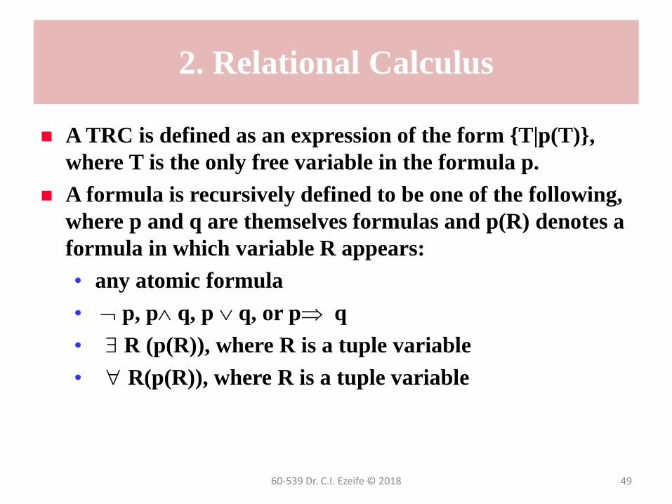
A TRC is defined as an expression of the form {T|p(T)},

where T is the only free variable in the formula p.

A formula is recursively defined to be one of the following,

where p and q are themselves formulas and p(R) denotes a

formula in which variable R appears:

• any atomic formula

• p, p q, p q, or p q

• $ R (p(R)), where R is a tuple variable

• " R(p(R)), where R is a tuple variable

60-539 Dr. C.I. Ezeife © 2018 49


Let op denote an operator in the set {<,>,=,<=,>=,!=}, an atomic formula is one of the following:

• R Rel , R.a op S.b, R.a op constant or constant op R.a(where R and S are relations and a, b are attrs)

A free variable is a variable that does not contain $ or " .

The expressive power of relational algebra is used as a metric of how powerful a relational database query language is.

A query lang. is said to be relationally complete if it can express all queries expressed by relational algebra.

60-539 Dr. C.I. Ezeife © 2018 50

2. Views

Views are tables that are defined in terms of queries over other tables

and its rows are not generally stored explicitly in the database but

computed from definition.

The view mechanism can be used to create a window on a collection of

data that are of interest to a group of users, and it provides logical data

independence since changes in the base tables do not affect the view

design.

The following query creates a view to find the names and ages of

sailors with a rating > 6, and include the dates.

• CREATE VIEW ActiveSailors(name, age, day)

AS SELECT S.name, S.age, R.day

FROM Sailors S, Reserves R

WHERE S.sname = R.sname AND S.rating > 6;

60-539 Dr. C.I. Ezeife © 2018 51

3. File Organization techniques

Data in a DBMS are stored on storage devices such as

disks and tapes.

The file manager issues requests to disk manager to

allocate or free space for storing records in units of a page

(4KB or 8KB).

The file manager determines the page of a requested

record and requests that this page be brought to the buffer

pool (part of memory) by the buffer manager.

The disk composition is shown in the following figure.

60-539 Dr. C.I. Ezeife © 2018 52


60-539 Dr. C.I. Ezeife © 2018 53

Structure of a Disk

spindle

Disk block

cylinder

tracks

a platter

Disk

arm Disk head

rotationArm movement


The time to access a disk block is:

Seek time + Rotational delay time + Transfer time

Seek time is the time to move disk heads to the track on

which a desired block is located.

Rotational delay is the waiting time for the desired block to

rotate under the disk head.

Transfer time is the time to actually read or write the data

in the block once the head is positioned.

To minimize disk I/O time, records should be stored such

that frequently used records be placed close together.

60-539 Dr. C.I. Ezeife © 2018 54


The closest we can place two records on disk is on the same

block, or then on the same track, same cylinder or adjacent

cylinder in decreasing order of closeness.

Pages of records are stored on disk and brought up to

memory when any record in them are requested by a

database transaction.

Thus, the disk manager organizes a collection of sequential

records into a page.

Higher levels of DBMS code treat a page as a collection of

records and a file of records may reside on several pages.

How can pages be organized as a file?

60-539 Dr. C.I. Ezeife © 2018 55


The possible file organization structures are:

• 1. Heap files: keep unordered data in pages in a file

(called heap file). To support inserting, deleting a

record, creating and destroying files, there is need to

keep track of pages in a heap file using doubly linked

list of pages or a directory of pages.

• 2. Ordered files: records are stored in an order in data

pages of the file.

• 3. Indexes: a file of ordered records for quickly

retrieving records of the original data file.

60-539 Dr. C.I. Ezeife © 2018 56

3. Indexes

Assume we have a database file of 1 million records with structure (student id, name, gpa), to get the students with gpa > 4.0, we need to scan the 1 million records. Slow approach.

A way to speed up processing of queries is build an index on the gpa attribute and store as an index file, which stores the records in gpa order.

An index is an auxilliary data structure that helps to find records meeting a selection condition.

Every index has an associated search key, a collection of one or more fields of the file we are building the index on; any subset of the field can be a search key.

Indexed file speeds up equality or range selections on the search key and quick retrieval of records in index file is done through access methods.

60-539 Dr. C.I. Ezeife © 2018 57

3. Indexes

Examples of access methods (organization techniques for index files) are B+

trees, hash-based structures

A database may have more than one index file.

A clustered index has its ordering the same or close to the ordering of its data

records in the main database. E.g., index on student id is clustered while that

on gpa is unclustered.

A dense index contains at least one data entry for every search key value that

appears in a record in the table.

A non-dense or sparse index contains one entry for each page of records in the

data file.

A primary index includes the primary key as its search key while a secondary

index is an index defined on a field other than the primary key.

60-539 Dr. C.I. Ezeife © 2018 58

3. Indexes

Tree-Structured Indexing

Assume we have the students file sorted on gpa,

To answer the range query “Find all students with gpa

higher than 3.0”, we identify the first such student by

doing a binary search of the file and then scan the file from

that point on.

An ISAM tree is a static structure which is effective when

the file is not updated frequently.

B+ tree is a dynamic structure that adjusts to changes

(addition and deletion) in the file gracefully.

60-539 Dr. C.I. Ezeife © 2018 59

3. Indexes

B+ tree supports equality and range queries well

In ISAM index structure there are data pages, index pages

and overflow pages.

Each tree node is a disk page and all the data reside in the

leaf pages.

At file creation, leaf pages are allocated sequentially and

sorted on key value. Then, the non-leaf pages are allocated.

Additional pages needed because of several inserts are

allocated from an overflow area.

60-539 Dr. C.I. Ezeife © 2018 60

3. Indexes (ISAM)

60-539 Dr. C.I. Ezeife © 2018 61

The basic operations of insert, delete and search are

accomplished by searching for the non-leaf node less

or equal to the search key and following that path to a

leaf page where data is inserted, deleted or retrieved.

An overflow page may need to be checked.

10* 15* 20* 27* 33* 37* 40* 46* 51* 55* 63* 97*

40

20 33 51 63

23*

Non-leaf

leaf

Overflow pages

An ISAM tree

3. Indexes (ISAM)

An insert operation of record 23 causes an overflow page since each leaf page holds only 2 records. Inserts and deletes affect only leaf pages

Number of disk I/O is equal to the number of levels of the tree and is logF P where P is the number of primary leaf pages and F is the fan out or number of entries per index page. N is P * F.

This is less than number of disk I/O for binary search, which is log2 N or log2 (P * F) . E.g., with 64 entries, 32 pages and 2 entries per page, ISAM’s disk I/O is 5 while binary search disk I/O is 6.

60-539 Dr. C.I. Ezeife © 2018 62

3. Indexes (B+trees)

B+ tree search structure is a balanced tree in which the

internal nodes direct the search and the leaf nodes contain

the data entries.

Leaf pages are linked using page pointers since they are not allocated

sequentially.

Sequence of leaf pages is called sequence set.

It requires a minimum occupancy of 50% at each node except the root.

If every node contains m entries and the order of the tree (a given parameter

of tree) is d, the relationship d m 2d is true for every node except the root

where it is 1 m 2d.

Non-leaf nodes with m index entries contain m+1 pointers to children.

Leaf nodes contain data entries.

60-539 Dr. C.I. Ezeife © 2018 63

3. Indexes (B+trees)

60-539 Dr. C.I. Ezeife © 2018 64

Insertion of 8 into the tree leads to a split of leftmost leaf node as well as

the split of the index page to increase the height of the tree.

Deletion of a record may cause a node to be at minimum occupancy and

entries from an adjacent sibling are then redistributed or two nodes may

need to be merged.

13 17 24 30

2* 3* 5* 7* 14* 16* 19* 20* 22*

24* 27* 29* 33* 34* 38* 39*

A B+ tree of height 1, order d=2

3. Multidimensional Indexes

B+ tree is an example of a one-dimensional index which allows linear

order to be imposed on the set of search key values.

Multidimensional indexes do not impose a linear order. However, each

key value is seen as a point in a k-dimensional space with k the number

of fields in the composite key.

E.g., in a 2-dimensional space of <age,sal>, a one dimensional index

maintains the key first in age order, then sal order to obtain a list like

<11, 80>, <12, 10>, <12, 20>, <13, 75>.

A multidimensional index stores data entries that are close together in

the k-dimensional space, close together on pages.

A more likely order is <12, 10> and <12, 20> together and <11, 80> and

<13, 75> together. R tree is a multidimensional tree-structured index

for storing geometric objects like regions.

60-539 Dr. C.I. Ezeife © 2018 65

3. Hash-based Indexing

60-539 Dr. C.I. Ezeife © 2018 66

Good for equality selection but poor for range selection

A hash function is used to map values in a search field into a range

of bucket numbers to find the page on which a desired data entry

belongs.

With static hashing, data pages are a collection of buckets with one

primary page and possibly additional overflow pages per bucket.

A file consists of buckets 0 to N-1 with one primary page per

bucket initially.

key h

0

1

:

N-1Primary bucket pages overflow pages

3. Hash-based Indexing

To search for a data entry, we apply a hash function h to

identify the bucket to which it belongs and search this

bucket.

Number of buckets is fixed, so that if a file grows, long

overflow chain may develop resulting in poor performance.

Extendible hashing uses a directory to support inserts and

deletes efficiently without overflow pages.

60-539 Dr. C.I. Ezeife © 2018 67

3. System Catalogs

A DBMS maintains information about every relation,

index, views that it contains which are stored in a collection

of relations called system catalog.

System catalog has information about each relation

• its name, filename, file structure

• name and type of each of its attributes

• index name of each index on the table

• integrity constraints, number of tuples

• name and structure of the index

• for each user, accounting and authorization information.

• Etc.

60-539 Dr. C.I. Ezeife © 2018 68

4. Query Optimization and Evaluation

Queries are parsed and then presented to a query optimizer which is responsible for identifying an efficient execution plan for evaluating the query.

The goal of a query optimizer is to find a good evaluation plan for a given query.

A query evaluation plan consists of an extended relational algebra tree with annotations indicating the access methods to use for each relation and the implementation method to use for each relational operator.

Result sizes may need to be estimated and the cost of the plans estimated.

The goal of a query optimizer is to find a good evaluation plan for a given query.

60-539 Dr. C.I. Ezeife © 2018 69

5. Database Design and Tuning model

The steps in database design are:

1. Requirements analysis: information about environment gathered

2. Conceptual Design: Presents a high-level description of data and

relationship between data entities. The second part of the conceptual

design is schema refinement guided through the powerful theory of

normalization.

3. Physical Database Design: Here indexes are built on relations, etc.

4. Database Tuning: Uses interaction between 3 steps above to achieve

better performance.

60-539 Dr. C.I. Ezeife © 2018 70


60-539 Dr. C.I. Ezeife © 2018 71

Schema Refinement and Normal Forms

Schema refinement in relations is an approach based on

decomposition of relations.

This is intended to address problems caused by redundant storage

of information which are: wasting storage, update anomalies,

insertion anomalies and deletion anomalies.

Ssn name lot rating wage hours

123-22-3666 Attishoo 48 8 10 40

231-31-5368 Smiley 22 8 10 30

131-24-3650 Smethurst 35 5 7 30

434-26-3751 Guldu 35 5 7 32

612-67-4134 Madayan 35 8 10 40

Hourly-Emps Relation


Assume that wage attribute is determined by rating

attribute. And if same rating appears in the rating column

of two tuples, then same value must appear in the wage

column.

Since rating 8 corresponds to wage 10, this information is

repeated. If we change wage for tuple 1 to 9, this is update

anomaly. We can not insert a tuple for an employee unless

we know her hourly rating, which is insertion anomaly.

If we delete all tuples with given rating, we lose the association between

rating value and wage (deletion anomaly)

60-539 Dr. C.I. Ezeife © 2018 72


Functional dependencies and other integrity constraints

force an association between attributes that may lead to

redundancy.

Many of the problems of redundancy can be eliminated

through decomposition of relations guided by the theories

of normal forms.

E.g., the Hourly-Emps relation can be decomposed into the

following two relations.

• Hourly-Emps2(ssn, name, lot, rating, hours)

Wages(rating, wages)

60-539 Dr. C.I. Ezeife © 2018 73


For a non-empty set of attributes X, Y in R, functional dependency FD:

X Y is read as X functionally determines Y and is true if the following holds for every pair of tuples t1 and t2 in r.

if t1. X = t2. X, then, t1. Y = t2 . Y

Note that both sides of an FD contain sets of attributes

A set of FD’s implied by a given set of FDs is called the closure of F denoted as F+.

The Armstrong’s axioms can be applied repeatedly to infer all FD’s implied by a set F of FDs. The Armstrong axioms are:

1. Reflexivity: if X Y, then X Y

2. Augmentation: if X Y , then XZ YZ for any Z

3. Transitivity: if X Y and Y Z , then X Z

60-539 Dr. C.I. Ezeife © 2018 74


Other rules satisfied are:

• Union: if X Y and X Z , then X YZ

• Decomposition: if X YZ and X Y , then X Z

The normal forms based on FDs are first normal form (1NF), second (2NF), third (3NF) and Boyce-Codd normal form (BCNF)

A relation is in 1NF if every field contains only atomic values.

Let A be an attr of relation R and X, a subset of attrs of R. R is in

BCNF if for every FD X A that hold over R, one of the following statements is true:

• A X, that is, it is a trivial FD or

• X is a superkey (a set of fields that contain a key)This means that every determinant is a candidate key and prevents forming relations with multiple composite keys that overlap.

60-539 Dr. C.I. Ezeife © 2018 75


R is in 3NF if for every FD X A that holds over R:

• A X, that is, it is a trivial FD or

• X is a superkey (a set of fields that contain a key)

• A is a part of some key for R.

That is, if every non-key attribute is non-transitively dependent on the primary key.

Other types of dependencies are multivalued dependencies (MVD) and join dependencies (JD) and Inclusion dependency.

A relation is in 4NF if for every MVD X Y that holds over R:

Y X or XY= R or X is a superkey (ie has no MVDs except as spcified).

A relation R is in 5NF if for every JD that holds over R one of the following is true: join of Ri = R for all i, or

• JD is implied by the set of those FDs over R where left side is a key.

That is, if a join of relations Ri gives back R without any loss of a tuple.

60-539 Dr. C.I. Ezeife © 2018 76

5. DBMS Benchmarks

A DBMS benchmark is a system of programs and queries for

evaluating the performance of a DBMS

A DBMS workload consists of a mix of queries and updates.

By testing the same set of workoads on a number of DBMS’s,

performance parameters like number of transactions per second, price

per performance ratios are gathered for each DBMS to guide users on

which DBMS is most suited for their needs.

E.g., Transaction Processing Council (TPC) TPC-A, TPC-B and TPC-

C (for warehouse). TPC-D benchmark (for decision support

applications). The 001 and 007 benchmarks measure performance of

object relational database systems.

60-539 Dr. C.I. Ezeife © 2018 77

6. Transaction Processing

Concurrency control and Recovery

A transaction is a DML statement or a group of statements that

logically belong together.

The group of statements is defined by two commands:

COMMIT and ROLLBACK in conjunction with the SAVEPOINT

command.

An interleaved execution of several transactions is called a schedule.

An execution of a user program or transaction is regarded as a series

of reads and writes of database objects.

The important properties of database transactions are ACID for

atomicity, consistency, isolation and durability.

60-539 Dr. C.I. Ezeife © 2018 78

6. Transaction Processing

Assume we have two transactions T1 and T2, defined as follows:

• T1: R1(A), W1(A), R1(C), W1(C)

• T2: R2(B), W2(B)

A schedule for running T1 and T2 concurrently should produce the

same effect as running T1, T2.

One such schedule is:

• R1(A), W1(A), R2(B), W2(B) , commit(T2), R1(C), W1(C),

commit(T1)

Approaches for concurrency control include (1)strict two-phase

locking (strict 2PL), (2) 2 Phase locking, serializability and

Recoverability, (3) View Serializability, (4) Optimistic concurrency

control and (5) Timestamp-based concurrency control.

60-539 Dr. C.I. Ezeife © 2018 79

6. Crash Recovery

The recovery manager is responsible for atomicity (ensuring that

actions of uncommitted transactions are undone) and durability

(ensuring that actions of committed transactions survive system

crashes and media failures).

It keeps a log of all modifications on stable storage. The log is used to

undo the actions of aborted and incomplete transactions and to redo

the actions of committed transactions.

DATABASE SECURITY

Issues of interest in a secure database are secrecy, integrity and

availability

Secure policy and mechanisms are needed to enforce this

60-539 Dr. C.I. Ezeife © 2018 80

6. Database Administrator

Role of the Database Administrator (DBA) are:

• 1. Creating new accounts

• 2. Mandatory control issues: must assign security

classes to each database object and security clearance to

each authorization id in accordance with the chosen

security policy.

• 3. Maintaining Audit trail: log of updates or all actions,

etc.

60-539 Dr. C.I. Ezeife © 2018 81

PART 2 : DATA WAREHOUSING

1. Components of a Data Warehouse

Operational Source databases

Operational Data Store

Data Warehouse Data and Meta Data

2. Building a Data Warehouse

Data Extraction, cleaning and Transformation

tool(ETL)

Front end tools (EIS, OLAP, DATA MINING)

3. Warehouse Database Management Schemas

4. Research Issues in Data Warehousing

60-539 Dr. C.I. Ezeife © 2018 82

1. Components of Data Warehouse

60-539 Dr. C.I. Ezeife © 2018 83

sdb1 sdb2 sdb3

Data WarehouseMeta

data

EIS OLAP Data mining DSS Warehouse admin & others

Operational source dbs

ODS

Data Extraction, cleaning

and loading tool

Data transformation tool

Warehouse Architecture including an ODS

1. What is a Data Warehouse?

A Data Warehouse is:

• a large database organized around major subjects

(entities) of an enterprise (not around functions).

• an integrated database collecting data from a number

of source application databases.

• a historical database system representing data over a

long time horizon (up to ten years).

• a database that supports online analytical processing

(OLAP) for decision support systems.

• A mostly non-changeable collection of data.

60-539 Dr. C.I. Ezeife © 2018 84

1. Warehouse Example

60-539 Dr. C.I. Ezeife © 2018 85

Consider a simple banking warehouse system where

there is an integration of two application source

databases keeping track of all transactions in the

following two source databases (1) a Savings account

db, and (2) a Checking account db.

custid transtype Amount

C0001 dep 500

C0518 wd 200

C0300 dep 300

cid trans amt balance

0518 wd 100 400

0001 dep 200 600

Customer(custid, name, address)

Balance(custid, balance)

Transaction(transtype, trname)

Savings source database S1 Checking source db C1

Customer(cid, name, address)

Transaction(trans, trname)


Source databases hold current data which are periodically populated to the warehouse.

The following warehouse fact table represents an integration of more than one source databases.

• B-activity (cid (C), acctcode (A), transtype (T), time-m (I), amt)

Since the fact table is made up of foreign key attributes, dimension tables which specify the dimension attributes are also kept

• Customer(cid, cname, ccity, cphone)account(acctcode, accttype, date-opened),time (time-minute, hour, day, mm, yy)

60-539 Dr. C.I. Ezeife © 2018 86


60-539 Dr. C.I. Ezeife © 2018 87

A sample fact table from integrating 4 such source accounts (S1, S2, C1,

C2) is:

cid acctcode transtype time-m Amount

C0001 S1 dep 199603210003 500 *

C0518 C1 wd 199603210100 400

C1000 C2 wd 199603210200 300

C0001 S1 dep 199603221300 500

C0518 S2 dep 199603230600 300

C0411 S2 dep 199603230600 400

C1000 C2 wd 199603231000 100

C0300 S1 dep 199603231200 300

C0411 C2 dep 199603240500 400

C0001 C1 wd 199603210003 600

The time is recorded as yy/mm/dd/minute with last 4 digits used for

Both minute and hour since there are 1440 minutes in a day.


This integrated, historical, subject-oriented, non-volatile database provides means for executives to achieve business goals (increasing market share, reducing costs and expenses, and increasing revenues).

Some Warehouse queries are:

• (1) Get the number of customers who have made more than 2 withdrawals in savings account “S1” in any month

• (2) Get the number of customers who have deposited some money in the morning minutes

• (3) Find the total amount of money involved in each transaction type and account type during lunch hour (0720 and 0780)

• (4) Find the total amount of money deposited by each customer every minute in account C1.

60-539 Dr. C.I. Ezeife © 2018 88

1. Why Data Warehouse?

Business enterprises (e.g., a telephone company) need to

find ways to gain competitive advantage over rival

companies. Data Warehousing is needed because:

• 1. Decisions need to be made quickly and correctly using all

available data, the amount of which increases tremendously within

a few weeks.

• 2. Competitor has figured ways to analyze their data quickly and

might steal enterprise clients.

• 3. There is hardware technology to exploit (can handle large data

and processing fast).

• 4. Legacy systems already owned by enterprise can be integrated.

60-539 Dr. C.I. Ezeife © 2018 89


Areas Business want IT to provide some information on are:

• 1. Customer retention: identify likely defectors and offer excellent deals to keep them.

• 2. Sales and Customer Service: identify products bringing in most profits and those most needed by customers

• 3. Marketing: Discovering market trend by getting information about competitor’s trend.

• 4. Risk assessment and fraud detection: E.g. discovering questionable transactions.

• 5. Classification: Using customer classification to set operational

rules.

60-539 Dr. C.I. Ezeife © 2018 90


• 6. Clustering and Segmentation: Used to segment a database into

subsets or clusters based on attributes. Clusters can be analyzed

statistically by a program or by using visualization techniques.

• 7. Associations: Used to identify product affinities or products that

are needed together.

• 8. Sequencing: used to identify sequences of transactions that

customers ask for together.

To provide needed solution to business, data warehouses are used to

integrate internal and external data into a comprehensive view

encompassing the whole organization.

Data mining application can be used to mine the integrated data for

information.

60-539 Dr. C.I. Ezeife © 2018 91

1. Source Databases and Warehouse

Warehouse data represent integration of data from a number of data

sources in the form of flat files, relational databases, object-oriented

databases etc.

Different source data may be operating on different hardware and

software platforms. It is the responsibility of the transformation tool

(called extraction, transformation and Loading or ETL tool) to convert

data on these platforms to a uniform platform where the data

warehouse or operational data are stored.

Data in the warehouse can be organized at different levels of detail

namely: current level detail data (e.g. up to one week/month old), old

level data (eg. Longer than one week/month) and summarized data (e.g

as views through aggregate functions).

60-539 Dr. C.I. Ezeife © 2018 92

1. Source Databases and Warehouse

60-539 Dr. C.I. Ezeife © 2018 93

Differences between Data Warehouses and Source Databases.

Feature source DB Warehouse data

Data content current values summarized, archived & derived,

integrated

Data organization by application by subject

Data stability dynamic static until refreshed

Data structure optimized for transaction optimized for complex queries

Access frequency High medium to low

Access type Read/update/delete Read/aggregate/added to

Usage Predictable, repetitive ad hoc, unstructured, heuristic

Response time subsecond (< 1 sec) to 3s several seconds to minutes

1. Data mart and Metadata

A data mart is a warehouse customized to suit the needs of

a particular department owning the data. A collection of

data marts composes an enterprise-wide data warehouse.

Metadata is data about data and has such information as

the location and description of warehouse system

components, contents of the data warehouse and end-user

views, integration and transformation rules, history of

warehouse updates etc.

60-539 Dr. C.I. Ezeife © 2018 94

1. Operational Data Store (ODS)

Operational data store (ODS) is a smaller warehouse kept

for a shorter period of time before moving its data up to

the main warehouse.

ODS can be seen as a short term warehouse

ODS contains very current data while warehouse contains

both current and historical data.

ODS contains only detailed data and not the summaries or

aggregates while warehouse includes summaries.

The data warehouse architecture given includes the ODS

although it is optional.

60-539 Dr. C.I. Ezeife © 2018 95

1. Two-Tiered and Multitiered warehouse

architecture

In the two-tiered architecture, the client runs the EIS, DSS,

OLAP, data mining applications while the server maintains

the data warehouse.

A multi-tiered architecture lets the client run the EIS, DSS,

OLAP and data mining applications, but the client

communicates with application or data mart servers which

summarize, filter and maintain their own metadata’s.

These application servers in turn communicate with

warehouse server which maintains overall warehouse

metadata and file services.

60-539 Dr. C.I. Ezeife © 2018 96

2. Building the Data Warehouse

Involves the following tasks (similar to those for building a database

application):

• 1. Collecting and analyzing business requirements an designing

database tables (schemas)

• 2. Choosing the database technology and platform for the

warehouse (the DBMS server and clients).

• 3. Extracting data from operational source dbs, transforming,

cleaning and loading data in the wh.

• 4. Choosing data warehouse front end or Access tools for querying

warehouse data

• 5. Periodically updating the warehouse

• 6. Performance fine tuning through logical and physical warehouse

design.

60-539 Dr. C.I. Ezeife © 2018 97

2. Building the Data Warehouse

1. Collecting and analyzing business requirements: This

stage involves defining the problems that business wants

solved, the data they have available and their locations etc.

2. Choosing the database platform for the warehouse: This

decision is influenced by available resources. E.g., what

DBMS and hardware is available and can adequately

handle the volume of data to be integrated?

3. Extracting, transforming, cleaning and loading data into

the warehouse: This is major step which is discussed more

in detail next.

60-539 Dr. C.I. Ezeife © 2018 98

2. Data Extraction, Clean up and

Transformation Tools

Tasks to be performed by the tools are:

• Data transformation from one format to another, e.g.,

source db 1 represents gender of customer as ‘F’ and

‘M’ and another source db2 represents it as 1 for female

and 0 for male. The two sources have some differences

in schema definitions and one is stored on MS Access

while the other is stored on Oracle DBMS.

• Data consolidation and integration which includes

combining several source records into a single record to

be loaded into the warehouse.

60-539 Dr. C.I. Ezeife © 2018 99



• Metadata synchronization and management including storing data into and updating metadata.

Vendor Approaches to Data Extraction and Trans.

• 1. Code Generators: are transformation tools based on source and target data definitions, data transformation and enhancement rules defined by the developer. Code generation products are used for data conversion projects and for building an enterprise wide data warehouse. The approach generates a program for each group of data sources which copies data from source to target system.

60-539 Dr. C.I. Ezeife © 2018 100



• 2. Database Replication Tools: employ database triggers

or recovery log to capture changes to a single data

source on one system and apply the changes to a copy of

the source data at a different location. Effective for

building small ODS, warehouses involving a few

sources.

• 3. Rule-driven dynamic transformation engines:

capture data from a source system at user-defined

intervals, transforms the data and then sends and loads

the results into a target environment.

60-539 Dr. C.I. Ezeife © 2018 101



Data Extraction Tool Vendors

-. Some currently popular Extraction, Transformation

and Loading (ETL) tools are Informatica (power center),

IBM (Websphere datastage) and (Cognos Data Manager),

SAP (BusinessObjects data integrator), Microsoft (SQL

server integration services), Oracle (data integrator), SAS

(data integration studio), Oracle (data integrator), etc.

60-539 Dr. C.I. Ezeife © 2018 102

2. Data Warehouse Access Tools

Many of the warehouse access tools aim at providing graphical user interface (GUI) based mechanisms for querying and generating reports etc.

The tools can be:

• 1. Data query and reporting tools (eg. Built with Oracle forms or php)

• 2. Application development tools (eg. with SQL, ODBC, ADO.NET, JDBC, XML, XPath, Xquery).

• 3. Executive information system (EIS) tools

• 4. On-line analytical processing (OLAP) tools

• 5. Data Mining tools.

60-539 Dr. C.I. Ezeife © 2018 103


1. Query and Reporting tools : Reporting tools include

batch reporting tools using languages like COBOL,

Information Builders and desktop report writers like

Crystal Reports and forms.

2. Application development tools: used to create and view

standard reports, define and create ad hoc reports and for

data exploration. Many of the applications

60-539 Dr. C.I. Ezeife © 2018 104


have support for object linking and embedding (OLE),

object database connectivity (ODBC), and hypertext mark-

up language (HTML).

3. Executive Information System tools (EIS): EIS

applications highlight exceptions to normal business

activity. Popular EIS tools include Business Objects,

Hyperion, SAS/EIS, TRACk Business Solutions

60-539 Dr. C.I. Ezeife © 2018 105


4. Olap tools support aggregation of data through

hierarchies and dimensions. Users can drill down or up

levels in each dimension, pivot or swap out dimensions to

change their view of data. Some tools are Arbor Software’s

Essbase and Oracle’s Express, Cogno’s PowerPlay. Olap is

discussed further next.

5. Data Mining tools: Mining tools use a variety of

statistical and AI algorithms to analyze the correlation of

variables in the data and highlight interesting patterns and

relationships to investigate, e.g., WEKA miner, SAS data

mining solution, IBM’S quest, SGI Mineset etc.

60-539 Dr. C.I. Ezeife © 2018 106

2. OLAP

4. OLAP tools

Modern business problems are characterized by the need

to retrieve large number of records from very large data

sets and summarize them.

There is need to do such things as market analysis and

financial forcasting which require schemas that are array-

oriented and multidimensional in nature.

The two-dimensional relational model has some speed

limitations for such complex real-world problems.

60-539 Dr. C.I. Ezeife © 2018 107

2. OLAP

• for example, a query may translate into a number of

complex SQL statements, each of which may require

full table scan, multiple joins, aggregations and large

temporary tables for storing intermediate results.

• SQL does not support grouping by an aggregate

function since Select amt from fact group by sum(amt)

is illegal.

OLAP uses a multidimensional model to provide a solution

which also supports drill-down and roll-up analysis.

60-539 Dr. C.I. Ezeife © 2018 108

1. Drill-down and Roll-up analysis of the

warehouse

Warehouses allow business analysis to be performed either top-down (drill-down) fashion or bottom-up (roll-up) fashion.

Drill-down analysis starts providing the summarization of warehouse data at a highly summarized level before getting to the most detailed level. E.g., provide the total number of withdrawals by each customer every year, then every month, week, hour, …….., second.

Roll-up analysis starts providing the summarization at a most detailed level before gradually doing it at a highly summarized level.

Pivoting: provides aggregation on a set of dimensions, eg , CATI, ATIC by rotating the attributes to get alternative view of data

Slicing: is an equality selection on one dimension possibly with some dimensions projected out. E.g. select cid, sum(amt) from fact where fact.cid = C0518 group by acctcode, transtype;

Dicing: is a range selection on one or more dimensions. Eg. … where fact.time-m <= 1200 group by cid, acctcode.

60-539 Dr. C.I. Ezeife © 2018 109

2. Multidimensional Data model

Example of a multidimensional question is “how much revenue did the new product generate by month in the northeastern division, broken down by user demographic, by sales office, relative to the previous version of the product, compared with the plan?” - a six dimensional question.

The multidimensional data model is viewed as a data cube (a data model for presenting different or multiple perspectives of some aggregate measure value like total revenue).

The relational table given below has detailed sales data by product, market and time.

60-539 Dr. C.I. Ezeife © 2018 110


60-539 Dr. C.I. Ezeife © 2018 111

Product market time units

camera Boston Q1 1200




camera Seatle Q1 1000

camera Seatle Q2 1100

…………………………………..

tuner Denver Q1 250

tuner Denver Q2 300

Detailed sales data by product,

market and time.

market

product

timeQ1 Q2 Q3 Q4

Camera 1200 1500 1800 2100

BostonSeatle

Denver

Data Cube


The cube on the right associates sales numbers (units sold) with dimensions (product type, market and time) with the unit sold organized as cells in an array.

The dimension time has a hierarchy like quarter year.

The cube supports matrix arithmetic on cells of the array and the response time depends on the number of cells to be added on the fly.

Problem with this model is that the number of cells in the cube increases exponentially as the number of dimensions increases and

many queries need summarized high level data.

60-539 Dr. C.I. Ezeife © 2018 112


One solution to speed up performance is to pre-aggregate

all logical subtotals and totals along all dimensions.

Pre-aggregation allows for drill-down aggregation along

dimension hierarchies.

Another issue with the cube is how to handle sparse data

since not every cell has a meaning across all dimensions.

Relational OLAP (ROLAP) implements multidimensional

data cube using the relational data model with the Star or

snowflake schema.

60-539 Dr. C.I. Ezeife © 2018 113


60-539 Dr. C.I. Ezeife © 2018 114

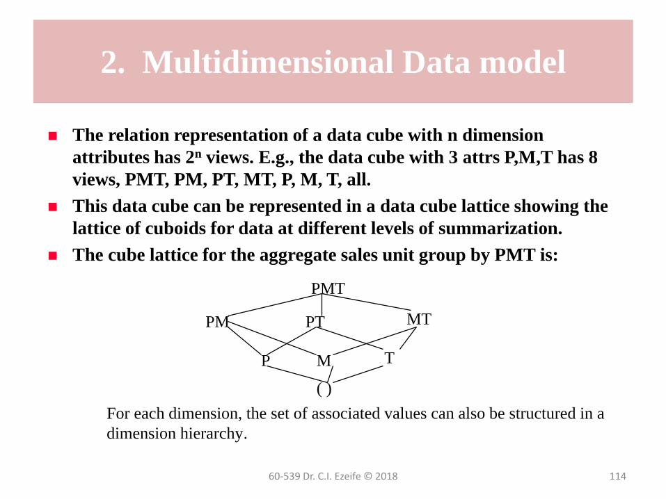
The relation representation of a data cube with n dimension

attributes has 2n views. E.g., the data cube with 3 attrs P,M,T has 8

views, PMT, PM, PT, MT, P, M, T, all.

This data cube can be represented in a data cube lattice showing the

lattice of cuboids for data at different levels of summarization.

The cube lattice for the aggregate sales unit group by PMT is:

PMT

PM PT MT

P M T

( )

For each dimension, the set of associated values can also be structured in a

dimension hierarchy.


Example ROLAP tools are Microstrategy (DSS Agent),

SAP Business objects, Oracle Business Intelligence,

Mondrian (open source).

Other OLAP tools implement the cube using array-like

structures and these are called MOLAP (multidimensional

OLAP). Examples are Cognos, Powerplay, Oracle

database olap option.

60-539 Dr. C.I. Ezeife © 2018 115

3. Warehouse DBMS Schemas

Star Schema

The most common schema methodology for data warehousing based

on the relational model is the star schema.

The star schema allows information to be classified into facts and

dimensions.

Facts are organized and stored in a fact table as foreign key attributes

and some measure attributes, e.g., customer id, transaction id, account

type, time-second.

Dimensions are stored in dimension tables as attributes describing the

facts, e.g.,

customer id, customer name, phone

time-second, minute, hour, day, month, year.

60-539 Dr. C.I. Ezeife © 2018 116


Dimension attributes define dimension hierarchies.

The facts are foreign key attributes to the dimension

tables.

The star schema simplifies answering multidimensional

queries like “Get the total number of withdrawals by each

customer every day, then every month and every year”.

A star schema is a relational schema organized around a

central table (fact table) using foreign key references.

60-539 Dr. C.I. Ezeife © 2018 117


60-539 Dr. C.I. Ezeife © 2018 118

Fact

cid

acctcode

transtype

time-m

Amt

Balance

customer

cid

cname

ccity

cphone

account acctcode

accttype

date-op

transaction

transtype

tname

timingtime-m

hour

day

month

year

THE STAR SCHEMA


60-539 Dr. C.I. Ezeife © 2018 119

A star schema can be created for every industry - consumer

packaged goods, retail, telecommunications,

transportation, insurance etc.

The dimension hierarchies from the schema above are:

cid

cname ccity cphone

acctcode

accttype date-op

transtype

tname

Time-m

hour

day

month

year


Alternative Warehouse Schema - Snowflake Schema

Snowflake schema is a variant of the star schema where some

dimension tables are normalized to reduce redundancies. Set back is

that for olap queries involving huge fact table, more table joins may be

expensive. E.g.,

fact(cid, ……)

customer(cid, cname,caddress, crating)

customerating(crating, loanpaidup)

Fact Constellation: This schema allows multiple fact tables to share

dimension tables. It is also called galaxy schema.

60-539 Dr. C.I. Ezeife © 2018 120


Some performance problems in warehouse design need

some improvement and these include:

1. Relational query optimizers have been optimized for OLTP

processing and thus multidimensional queries typical of warehousing

will not benefit from such optimizations.

2. Since the star schema has been somewhat denormalized and when

placed back on the relational DBMS, the result may be poor

performance.

3. Query Language: Thus, SQL needs to be extended to support such

OLAP operations as cube, drill-down, roll-up, etc. Some DBMSs like

Oracle 9i are already providing these support.

60-539 Dr. C.I. Ezeife © 2018 121


60-539 Dr. C.I. Ezeife © 2018 122

3. Indexing: Indexes can be used to speed up olap queries.

Efficient indexing techniques for olap need to be developed. Some

indexing techniques under use include bitmap and join indexing.

Example bit map index. Consider the Purchase table below(left)

cid item city

1 H V

2 C V

3 P V

4 S V

5 H T

6 C T

7 P T

8 S T

cid H C P S

1 1 0 0 0

2 0 1 0 0

3 0 0 1 0

4 0 0 0 1

5 1 0 0 0

6 0 1 0 0

7 0 0 1 0

8 0 0 0 1

cid V T

1 1 0

2 1 0

3 1 0

4 1 0

5 0 1

6 0 1

7 0 1

8 0 1

Purchase Relation item bit map city bit map


Every attribute of the table has a bitmap index where there is a distinct

bit vector Bv for each value v in the domain of the attr.

E.g., for attr. Item, there are 4 bit vectors for the attr values H, C, P, S.

Each bit vector is 8 bits long for the 8 records in the table.

For each record in the db table, the attr value the record has in the

table is set to 1 in its bit map index and the rest of the record’s bit

vectors are set to 0. E.g., record 1 purchased item H, while record 2

purchased item C and the item bit map shows the bit vector for record

1 as 1000 while that for record 2 is 0100.

Bitmap index leads to reduction in space and I/O and is useful for low

cardinality domains because comparisons, join and aggregation

operations are reduced to bit arithmetic.

60-539 Dr. C.I. Ezeife © 2018 123


Join Index: Traditional index maps the value in a given column to a list

of rows having that value.

On the other hand, join indexing registers the joinable rows of two

relations from a relational database. Eg. Join index for product/market

from pmt fact table may record the tuples (camera, Boston), (camera,

Seatle), (tuner, Denver).

Assume there are 360 products, 10 city markets, and 10 million sales in

the fact. If Sales have been recorded for only 3 markets, the other 7

markets will not participate in the join.

Bit map and Join indices can also be used combined.

Exploring the use of these and new indexing techniques for speeding

up warehouse queries remain research issues.

60-539 Dr. C.I. Ezeife © 2018 124


4. Materialized View and Online Aggregates: While materialized views are precomputed aggregate view used to speed up query responses, online aggregation provides approximate answers and continues with user’s interaction in a direction. Methods researched include partitioning and indexing and maintenance of materialized views. Reducing time for updating warehouse fact table and views is important and many algorithms have been proposed for maintenance of materialized views and open problems still exist in this area.

5. Data Cleaning Techniques: Providing high quality data in warehouses is accomplished by efficient and reliable data cleaning techniques.

7. Integration of warehousing processes with mining such that mining systems can extract, integrate, clean, and analyze data.

60-539 Dr. C.I. Ezeife © 2018 125


8. Increasing usability of warehousing system is achieved by making the process of building wh systems cheaper and easier, techniques for integrating data sources through code generation are being incorporated by some dbmsvendors. Efficiently managing and maintaining metadata is an important research issue.

Building extraction tools that can uniformly apply to a number of different types of data sources will cut down on coding and thus on the price of the product and is being investigated.

60-539 Dr. C.I. Ezeife © 2018 126

PART 3 - DATA MININING

1. Data Mining Techniques

1. 1 Association Rule Mining

1.2 Classification and Regression Rules

Decision Trees

1.3 Clustering

1.4 Genetic Algorithms

2. Data Visualization

60-539 Dr. C.I. Ezeife © 2018 127

1. Data Mining

Data mining helps end users extract useful business information from

large databases.

Data mining is used for finding interesting trends or patterns in large

datasets to guide decisions about future activities.

Data mining helps answer questions like

• 1. What has been going on in my data?

• 2. What is going to happen next?

• 3. How can I profit?

Data mining tools provide solutions which are built on such computer

algorithms as association rule mining, decision tree classifications,

neural networks, and clustering techniques like nearest neighbor.

60-539 Dr. C.I. Ezeife © 2018 128

1. Data Mining

Data mining is closely related to the area of statistics called exploratory data analysis and also related to the subareas of artificial intelligence called knowledge discovery, but handles much larger data in an automated fashion.

Data mining tools are built to be embedded into the business data warehouse and to be understandable and usable by marketing professionals, while classic statistical tools can not fulfil these objectives.

Data mining is used for information discovery (looking for gold in mountain of data) and prediction (using the found information gold to predict what will happen next)

The knowledge discovery and data mining (KDD) process consists of data selection, data cleaning, data mining and result evaluation.

60-539 Dr. C.I. Ezeife © 2018 129

1. Data Mining

The importance of the discovered information can be

measured by (1) how strong the association is and (2) how

unexpected

Two ways for building predictive models are called

supervised learning and unsupervised learning.

With supervised learning, the aim is to predict some target

field in the historical database, unsupervised learning has

no well-defined goal or target to predict.

Techniques such as clustering and detection of association

rules fall into the category of unsupervised learning.

Mining techniques are discussed next.

60-539 Dr. C.I. Ezeife © 2018 130

1.1 Association Rule Mining

Association Rule mining is the most common form of knowledge discovery in unsupervised learning systems.

Mining for gold in this method is equivalent to looking for an interesting rule, formed from database attributes occurring strongly together in the same transactions.

Association Rule mining in a database aims at pulling out all possible patterns (combinations of attributes) from the database, calculating their support (or coverage) and confidence (accuracy).

Rules are generally simple, e.g.,

“If bagels are purchased, then cream cheese is purchased 90% of the time and this pattern occurs in 3% of all shopping baskets.”

60-539 Dr. C.I. Ezeife © 2018 131


Where is Association Rule Mining Used?

Examples of rules are

• if paper plates,then plastic forks (paper plates => plastic forks)

• if dip, then potato chips(dips => potato chips)

• if salsa, then tortilla chips (salsa => tortilla chips)

For the computed rules to be useful, two pieces of information must be

supplied by the mining result as well:

• 1.Confidence (accuracy): how often is the rule correct?

• 2. Support (or Coverage) : how often does the rule apply?

The rules themselves consist of two halves, the left side called

antecedent and right side called consequent.

60-539 Dr. C.I. Ezeife © 2018 132


60-539 Dr. C.I. Ezeife © 2018 133

Example of Rule confidence and support

The first rule is a pattern that occurs quite often and is right more

often than not, while the last rule is almost never wrong but also is

almost never applicable.

The antecedent can consist of one or multiple conditions which

must all be true in order for the consequent to be true at the given

confidence (accuracy).

Generally, the consequent is a single condition.

Rule Confidence Support

if breakfast cereal, then milk is purchased 85 20

if bread purchased, then Swiss cheese purchased 15 6

if 42 years old and purchased pretzels and dry

roasted peanuts, then bear is purchased 95 0.01


60-539 Dr. C.I. Ezeife © 2018 134

What can business do with a rule?

1. Target the antecedent: E.g., collect all rules that show a certain

value (e.g., nail) on the antecedent to determine its relationship

with other items.

2. Target the consequent: E.g., place rules showing items in

consequent close to items as sales promo.

3. Target based on confidence: target highly accurate rules of 80 to

90% for higher benefit.

4. Target based on support: increased support means most readily

applicable.

5. Target based on interestingness: Interesting rules have high

confidence and high support and deviate from the norm.


General idea

Rules are created to show events in the database and are used to find interesting patterns in the database. The two important features of a rule are:

• 1. Confidence: the probability that if the antecedent is true, then the consequent will be true. High confidence means that this is a rule that is highly dependable. That is, confidence = |Rule|/|antecedent|

• 2. Support: the number of records in the database that the rule applies to. High support means that the rule can be used very often. That is,support = |Rule|/|total|

• Coverage: |antecedent|/|total| is also used in place of support sometimes.

60-539 Dr. C.I. Ezeife © 2018 135


In statistics, support is apriori probability of both the antecedent and consequent occurring and the confidence is the probability of the consequent conditional on the antecedent.

Thus, to calculate for a simple rule like “ if milk, then egg”milk eggTotal = 100 = total number of shopping baskets in the database.Egg = 30 = number of baskets with eggs in themMilk = 40 = number of baskets with milk in themBoth = 20 = number of baskets with both eggs and milk in themConfidence = |Both| = 20 = 50%

|Milk| 40

Coverage = |Milk| = 40 = 40%|Total| 100

Support = |Both| = 20 = 20%|Total| 100

60-539 Dr. C.I. Ezeife © 2018 136


Other measures of usefulness include:

1. Support of a Rule as either percentage or number of records: percentage of times the entire rule occursSupport = |Both| = confidence * coverage

|Total|= |Both| * |antecedent|

|antecedent| |Total|or Support= |Both|

2. Support as number: used to capture support not as a probability or percentage but as the total number of records that match the given antecedent. Support number = |antecedent U consequent|.

3. Significance: compares given pattern to random chance. To compute significance, we find the probability that all events are independent and compare it with the support for the rule.

60-539 Dr. C.I. Ezeife © 2018 137


Association Rule Mining Algorithms include the Apriori

Algorithm and the Frequent Pattern Tree Algorithm.

Given a market basket database with a list of 5 items and

4 transactions, with minimum support of 2 trans:

C1= {milk, sugar, bread, salt, tea}

TID items Purchased

1 milk, sugar

2 milk, sugar, tea

3 milk, sugar, bread, tea

4 sugar, bread, salt, tea

60-539 Dr. C.I. Ezeife © 2018 138


The Apriori algorithm finds the set of frequent patterns (large

itemsets, Li) iteratively by computing the support of each itemset in the

candidate set Ci . During each ith iteration, it finds the ith large

itemsets (Li) from Ci, before computing the next (i+1) candidate set Ci+1

as Li apriori-gen join Li. It then, prunes itemsets from Ci+1 which have

any subset that are not already large. The process terminates when

either a Ci or Li is an empty set.

The apriori-gen join of Li with Li joins every itemset k of first Li with

every itemset n of second Li where n > k and first (i-1) members of

itemsets k and n are the same.

Example mining of the above table with the Apriori algorithm

proceeds as:

60-539 Dr. C.I. Ezeife © 2018 139


L1(large itemsets 1) = {milk, sugar, bread, tea}

C2 = L1 apriori gen L1 = {milk:sugar, milk:bread, milk:tea, sugar:bread, sugar:tea, bread:tea} after join and prune stages.

L2= {milk:sugar, milk:tea, sugar:bread, sugar:tea, bread:tea}

C3={milk:sugar:tea, sugar:bread:tea}

L3 ={milk:sugar:tea, sugar:bread:tea}

C4={empty set} and Apriori ends.

The discovered large itemsets L = L1 U L2 U L3.

Rules are formed from these large itemsets and only strong rules with confidence greater than or equal to minimum confidence are kept.

To form rules, from each each frequent pattern Li, obtain subsets and from each subset s, form a rule as s Li – s, where s is the antecedent and Li – s is the consequent.

60-539 Dr. C.I. Ezeife © 2018 140


Versions of the Apriori algorithm have been developed for

other kinds of mining including sequential and web mining

(check article references for details).

The Frequent Pattern (FP-tree) algorithm stores the

database information in an FP-tree which is used for

mining.

60-539 Dr. C.I. Ezeife © 2018 141


Details of the FP-tree and FP-growth algorithms can be found in references. Summary of the algorithm is:

1. Get the frequent 1-items F1 in descending order of support.

2. For each transaction t in DB, get frequent transaction ft as only items in F1 order.

3. Using the ft set, construct the FP tree with F1 header linkages.

4. Recursively mine (in suffix order) the FP tree by starting from the lowest item down the leaf on the tree and obtaining the conditional pattern bases of the suffix frequent pattern first. And the process continues by reconstructing an FP tree with conditional pattern bases that are frequent with count greater than or equal to minimum support as long as there is more than one node on the tree to continuously find prefix frequent patterns of the already found suffix patterns.

60-539 Dr. C.I. Ezeife © 2018 142


E.g. Info from a mailing campaign by an insurance company is:

InsuranceInfo(age:integer, cartype:string, highrisk:boolean)

We want to use this table information to identify rules that predict the

insurance risk of new insurance applicants whose ages and cartypes

are known.

E.g., if age is between 16 and 25, and cartype is either Sports or Truck,

then, the risk is high.

The attribute we want to predict (highrisk) is called the dependent

attribute. The other attrs are called predictor attributes (age and

cartype).

The general form of the types of rules we want to discover is:

P1(X1) ^ P2(X2) ^ … ^ Pk(Xk) Y = C

60-539 Dr. C.I. Ezeife © 2018 143


The Pi(Xi) are predicates that involve predictor attrs Xi.

Attributes can be either numerical (e.g., age) or categorical (e.g.,

cartype and highrisk).

If the dependent attr is categorical, the rule is called classification rule,

but it is regression rule if the dependent attr is numerical.

Thus, since highrisk is categorical, we have classification rule in our

example as:

( age <= 25) ^ (cartype {Sports, Truck}) highrisk = true

Support and confidence for classification and regression rules can be

defined as:

Support: for a rule C1 C2 is the %age of tuples that satisfy C1 ^ C2

Confidence: for a rule C1C2 is the %age of C1 tuples satisfying C2 too.

60-539 Dr. C.I. Ezeife © 2018 144


A decision tree is a graphical or tree representation of a collection of classification rules. Each internal node denotes a test on an attribute, each branch represents an outcome of the test and leaf nodes represent classes or class distributions. Decision trees are built or learnt from training data. A basic decision tree induction algm is ID3 (Fig. 7.3 of Han book) and another is C4.5.

In order to classify an unknown sample, the attribute values of the sample are tested against the decision tree. A path from root to a leaf node holding the class prediction for that sample is traced. Given a data record, the tree directs the record from the root to a leaf. Each internal node of the tree is labeled with a predictor attribute called splitting attribute.

The outgoing edges of an internal node are labeled with predicate that involve splitting attributes of the node.

The combined information about the splitting attr and the predicates on the outgoing edges is called the splitting criterion of the node.

Each leaf node of the tree is labeled with a value of the dependent attribute. E.g.,

60-539 Dr. C.I. Ezeife © 2018 145


60-539 Dr. C.I. Ezeife © 2018 146

Age

carType

<= 25 >25

Sedan Sports, Truck

A DECISION TREE EXAMPLE

NO

NO YES

Insurance Risk Decision Tree

- A decision tree represents a collection of classification rules, one for each

leaf node. The tree is usually constructed in 2 phases – the growth and the

prune phases. Several algorithms exist for making both stages efficient (ID3,

C4.5). Other classification techniques are Naïve Bayesian Classification,

which is based on Bayes theorem “The effect of an attr value on a given class

is independent of the values of the other attrs” (see section 7.4 for more).


Where are decision trees used?

Decision trees automate the process of hypothesis generation and

testing and handle data with little or no preprocessing. They have been

used in application areas ranging from medicine to game theory and

business.

It can be used for exploration of data set by looking at predictors and

values chosen for each split of the tree.

It can be used to preprocess data for other prediction algorithms by

creating a subset of possibly useful predictors in the first run of data.

It is a supervised learning that can be built from historical data.

60-539 Dr. C.I. Ezeife © 2018 147


Growing the Tree

The first step in the process is to grow the tree.

In growing the tree, the objective is to find the best possible question to ask at each branch point of the tree to come up with homogeneous leaves

In building the tree, decision tree algorithms look at all possible distinct questions that could break up the data set into segments that are homogeneous with respect to the prediction values. They pick the questions through heuristics or at random. An entropy-based measure may be used for selecting the test or decision attribute.

60-539 Dr. C.I. Ezeife © 2018 148


Classification and Regression trees (CART) pick the

questions by trying them all before picking the best one.

The decision tree stops growing when either of the

following 3 conditions occurs:

• 1. Segment contains only one record or algorithmically defined

minimum number of records.

• 2. Segment is completely organized into one prediction value.

• 3. The improvement in organization is not sufficient to warrant

making the split (e.g. splitting 90% of churners to get 89.99% does

not represent any progress).

60-539 Dr. C.I. Ezeife © 2018 149

1.3. Nearest Neighbor and Clustering

Other less developed classification methods include K-nearaestneighbor classification, genetic algorithms, rough set and fuzzy set approaches. K-Nearest neighbor is a prediction technique that is based on learning by analogy and is quite similar to clustering

The idea here is that in order to determine what a prediction value is in a new record, the user should look for records with similar predictor values in the historical or training database and use the prediction value from the record that is “nearest” to the unknown record. “Nearness” is defined in terms of Euclidean distance d(X,Y) = sqrt(∑n

i=1(xi – yi)2) between two points X=(x1, x2, .., xn) and Y=(y1,y2,

..yn)

For example, in order to predict a person’s income, use the income of his nearest neighbor.

Nearness in a database may consist of other factors like school attended by person, degrees obtained etc.

60-539 Dr. C.I. Ezeife © 2018 150


Clustering is used to partition a set of records into groups such that

records within a group are similar to each other. However, unlike

classification, the class label of each objet is unknown. Clustering

groups the data into classes or clusters where objects within a cluster

have high similarity in comparison to one another, but are very

dissimilar to objects in other clusters.

Each such group is called a cluster and similarity or dissimilarity

between records may be measured by a distance function.

Clustering techniques include partition-based (e.g. K-Means),

hierarchical (e.g. BIRCH), desnsity-based (e.g DBSCAN, LSC), grid-

based methods (e.g. STING).

E.g., Customerinfo(caddress: string, salary: real)

60-539 Dr. C.I. Ezeife © 2018 151


Clusters are used more for exploration and summarization than for prediction and have been used in pattern recognition, image processing and market research.

Clustering can be used to identify outliers or records that stick out

The K-means algm is on Fig. 8.1 and is summarized as:Input: number of clusters k and a database of n objectsOutput: a set of k clusters tha minimizes the squared erorr criterion.Method:1. arbirtarily choose k objects as the initial cluster centers2. repeat3. (re)assign each object to the cluster to which the object is most similar, based on the mean value of the objects in the cluster;4. update the cluster means by calculating the mean of objects in each

cluster.5. until no change;

60-539 Dr. C.I. Ezeife © 2018 152

1.4. Genetic Algorithms

Genetic algorithms are algorithms that dictate how

population of organisms should be formed, evaluated and

modified.

E.g., there is a genetic algorithm that determines how to

select organisms for sexual reproduction and another that

will determine which organisms to be deleted from the

population.

Genetic algorithm can be used to optimize a variety of data

mining techniques like neural networks and nearest

neighbor.

60-539 Dr. C.I. Ezeife © 2018 153

OTHER Mining Approaches to Possibly

Explore

Sequential Mining and Web Mining algorithms (e.g.,

PLWAP) using Web access pattern tree

AI approaches to Mining using Neural Networks.

Statistical approaches to Mining using point estimation,

Bayes theorem, hypothesis testing, regression and

correlation, similarity measures etc.

Data Stream Mining

Incremental Mining and incremental sequential mining

Presentation of Mining Results through data visualization

and other means.

60-539 Dr. C.I. Ezeife © 2018 154


Data visualization displays patterns in a way that can

easily be understood by humans.

Data visualization has to do with finding a mapping

between very high-dimensional spaces that exist in the

database or the predictive model and the two-dimensional

space that exists on the computer screen.

Three dimensional and higher dimensional spaces are

simulated through the 2-dimensional space making the

task of data visualization even harder.

Good data visualization allows the user the following key

abilities:

60-539 Dr. C.I. Ezeife © 2018 155


• 1. Ability to compare data

• 2. Ability to control scale (look from a high level or drill

down to detail).

• 3. Ability to map the visualization back to the detailed

data that created it.

• 4. Ability to filter the data to look only at subsets or

subregions of it at a given time.

60-539 Dr. C.I. Ezeife © 2018 156


Visualization is used in a number of places within data mining as

follows:

As a first-pass at the data mountain which is used to provide the user

some idea of where to begin mining.

As a way to display the data mining results and predictive model in a

way that is understandable to the end user.

As a way of providing confirmation that the data mining was

performed the correct way.

As a way to perform data mining directly through exploration analysis,

allowing the end user to look for and find patterns so efficiently that it

can be done in real time by the end users without using automated data

mining techniques.

60-539 Dr. C.I. Ezeife © 2018 157

60-539: Emerging non-traditional database systems (Data...

Documents

Transcript of 60-539: Emerging non-traditional database systems (Data...