Proceedings of the International Conference “Underwater Acoustic Measurements: Technologies &Results” Heraklion, Crete, Greece, 28th June – 1st July 2005

SIX YEARS OF TOMOGRAPHY OBSERVATION IN THE CENTRAL LABRADOR SEA

Tom Avsica, Uwe Sendb, Emmanuel Skarsoulisc

aLeibniz Institute of Marine Sciences, University of Kiel, Kiel, Germany bScripps Institution of Oceanography, University of California, San Diego, USA cInstitute of Applied and Computational Mathematics, FORTH, Heraklion, Greece

Tom Avsic, Leibniz Institute of Marine Science, Duesternbrooker Weg 20, 24105 Kiel, Germany. Fax: +49-431-600-17-4151, email: tavsic@ifm-geomar.de

Abstract: The Central Labrador Sea is an area of water-mass formation with a strong impact on the deep water of the Atlantic Ocean. Within the German SFB460 project a mooring array has been maintained since 1996 in the Central Labrador Sea. The measured data include time series of temperature and salinity at the mooring locations, and also acoustic travel-time data from tomographic transmissions between the moorings for the period 1997-2003. From the analysis of travel-time data horizontally averaged temperature profiles were obtained along ~150 km sections defined by corresponding moorings; for the routine analysis of travel-time data the matched-peak inversion approach was applied. The obtained heat-content results from the tomography experiment reveal a warming of 0.18°C in the upper 1800m over five years. By comparing the heat content (from acoustic measurements) to the surface heat flux (from meteorological measurements and models) an estimate of the horizontal heat flux (due to advection) can be obtained. The horizontal mean temperature variability can be interpreted in terms of a change in the Labrador Sea Water (LSW) volume and the corresponding formation rates. The obtained estimates for the volume of newly formed LSW ranges between 1013m3 to 7*1013m3 and formation rates up to 8 Sv.

Keywords: Acoustic Tomography, Labrador Sea, Matched-Peak Inversion, Acoustic Thermometry, Formation Rate, Heat Content

1. INTRODUCTION

Acoustics in the ocean has been studied for various proposes and on various time/spatial/frequency scales. Ocean acoustic tomography was introduced by Munk and Wunsch [1] as a remote-sensing technique for large-scale monitoring of the ocean interior

using low-frequency sound. Measuring the travel/arrival times of pulsed acoustic signals propagating from a source to a distant receiver through the water mass over a multitude of different paths, and exploiting the knowledge about how travel times are affected by the sound-speed (temperature) distribution in the water, the latter can be obtained by inversion.

Away from ocean's boundaries potential temperature (T) and salinity (S) can be assumed conservative – meaning that watermasses can be tracked through the ocean by its T-S values. In general watermass transformations (changes in T and/or S) occur at the sea surface where large heat and freshwater fluxes exist. Only very few regions in the world ocean are known to produce watermasses found at depths larger then 1000 m. The Labrador Sea is one of them. Strong cold and dry winter storms cause intense surface cooling driving deep convection of the surface waters – often to 2000 m. The watermass produced by these conditions is called the Labrador Sea Water (LSW).

The LSW forms the upper part of the North Atlantic Deep Water (NADW) which flows southwards in the Deep Western Boundary Current. The warm North Atlantic Current (NAC) transports warm surface waters back to the North to balance for the NADW export to the south. Without the NAC the Western Europe's climate would be colder. Without deep water formation in the North Atlantic the sea surface height in the North Atlantic would be higher with strong impact for the coastal regions [2].

Convection in the Labrador Sea is driven by surface heat loss, however other aspects, such as preconditioning and freshwater water anomalies, have also significant influence on the convection process (see [3] for an overview on open ocean convection). Fresh water released from ice melting in the Arctic could reduce the salinity of the surface water in the Labrador Sea and thus reduce LSW production. Indeed since 1996 convection depths were reduced compared to the first half of the 1990's. However Dickson [4] reported strong variations in the LSW production over the last 4 decades. Furthermore, the first half of the 1990's could have been years with exceptionally high LSW production rates (Kieke, personal comm.).

In this work some results from the acoustic observation of the deep convection and watermass formation activity in the central Labrador Sea over a period of six years (1997-2003) are presented.

2. EXPERIMENT

The Labrador Sea Tomography Experiment was conducted from August 1996 to September 2003 in the central Labrador Sea, see Fig. 1, as part of the German SFB460 project (TP A2). The tomographic array consisted of 3-4 moored instruments (sources and receivers) which were redeployed annually in late spring or summer. The acoustic sources were of Webb type emitting BPSK signals at 400 Hz. During the period 1998-99 the source mounted on the mooring K3 (Fig. 1) emitted at 250 Hz. There were 6 transmissions per day by each source over the 6-year duration of the experiment.

The sources and receivers were positioned at a nominal depth of 150 m as a result of an optimization study seeking to maximize the amount of sound-speed information to be recovered. Typical distances between mooring pairs (with high-quality data in terms of signal-to-noise ratio) ranged between 150 km and 330 km [5]. The exact transceiver positions were monitored with 3 transponders deployed around the base of each mooring (short baseline navigation, [6]).

In this paper we concentrate on data from two acoustic sections (K1-K2 and K1-K3) defined by the three mooring positions K1, K2 and K3 (Fig. 1). On the K1-K2 section acoustic tomography data exists from 07/1997 to 05/2002 whereas on the K1-K3 section it exists from 07/1997 to 05/2003 with missing data from 05/2000 to 06/2001.

Fig.1: Position of K1, K2 and K3 moorings deployed in the central Labrador Sea during

the period 1997 - 2003. Lines indicate acoustic propagation paths for which travel times of acoustic signals are used herein.

3. INVERSION

The sound speed profile in the Labrador Sea is of polar type, meaning that the SOFAR channel is at or near the surface and that the eigenrays tend to be reflected at the surface (Fig. 2). To invert acoustic travel times of eigenrays into sound speed and hence into temperature (having the largest influence on sound speed) a certain amount of a priori knowledge about the typical sound-speed variability of the probed region is required. The common assumption, that the observed travel-time fluctuations can largely be explained by the horizontally averaged field, reduces the sought sound-speed field from a 2-D section to a one-dimensional vertical profile. Thus, the variability is sufficiently described by a set of vertical sound-speed modes, which in our case were calculated from EOF analysis of all available CTD profiles collected during the different Labrador Sea cruises since 1990.

The matched-peak tracking (MPT) approach [7], which was used to invert the travel-time data iτ of the different eigenrays 1, ,i I= K , by-passes the explicit solution of the peak identification problem (association between model and observed travel times) and also accounts for the non-linear behaviour of travel times. Using the mean profile and the sound-speed modes mentioned above and assuming a range-independent ocean environment the sound-speed variability in the area of interest can be represented through a modal expansion

( ) ( ) ( )1

L

0 l ll=

c z = c z + f zϑ∑

where 0( )c z and ( ), 1, ,lf z l L= K denote the mean profile and the empirical orthogonal functions, respectively. The solution of the direct problem in ocean acoustic travel-time tomography leads to a set of model relations

Θ∈== ϑϑτ ,,...,2,1),( Iigii

r

nonlinear in general, between the parameter vector ϑr

and the arrival times iτ . These relation

can be linearized about a discrete set of background states ( )bϑr

to calculate arrival times on a fine grid of model states

( )

( )( )[ ].)()(

1

bll

L

l l

bib

iig ϑϑ

ϑϑτϑτ −

∂∂

+= ∑=

rr

The theoretical arrivals are allowed to associate with observed peaks if their time distance is smaller than a tolerance which depends on the particular peak, the background state, and the parameter discretization step. Accordingly, each discrete model state can explain (identify) a number of peaks in a particular reception. The population of model states that explains the maximum number of observed peaks are considered the more likely parametric descriptions of the particular reception, that can be described in terms of mean values and variances / inversion errors (MPT solution, see [7] for details).

Fig.2: Some typical eigenrays between K1 and K2 transceivers for winter conditions. The deepest ray has its lower turning point at ~1800m. All eigenrays reflect at the surface.

Background shading: Potential Temperature.

4. DATA

Assuming that the temperature along the K1-K2 section is representative for the whole convection region the heat content of the water resulting from the acoustic measurements can be combined with surface heat flux data to obtain horizontal heat-flux estimates (associated with horizontal advection and eddy flux). Surface heat-flux data for the area of the experiment are available from the U.S. National Centre from Environmental Prediction (NCEP). Still, on the basis of discrepancies observed in comparisons between NCEP data and direct measurements [8], [9] only radiation fluxes were taken here from NCEP, whereas the sensible and latent heat fluxes were recalculated using two different bulk formulae. The first approach is the one used by Isemer and Hasse in 1987 [10], whose suitability for the Labrador Sea was shown by Bumke [9]. The second calculation uses the CLIB model described in Renfrew 2002 [8]. The difference between the two approaches is 5 W/m2 - the surface heat fluxes resulting on Renfrew's model are considered slightly underestimated

(pers. comm. Jerome Cuny), whereas the original NCEP mean net surface heat flux is about 30W/m2 different from both calculations used herein.

For the LSW volume estimations knowledge over the LSW layer depth and the LSW temperature is needed. This data was obtained by analyzing simultaneously T-S mooring data, shipboard obtained CTD sections and TS-diagrams – a detailed description of the applied methods goes beyond the scope of this paper – and the results from this work are summarized in Table 1 (the interested reader can find more information on http://www.ifm-geomar.de/index.php?id=1468&L=1).

5. RESULTS

Tomography gives accurate horizontal mean temperature profiles. The heat content of the water along an acoustic section can directly be compared to surface heat flux to obtain the horizontal heat flux. If the vertical layer depth is such that it includes all the water which can exchange heat with the surface then the difference between the heat content and the surface heat flux has to be balanced by horizontal heat flux (similar to [11]).

Fig.3: Ocean's heat content along the K1-K2 section in the upper 1800m and the net

surface heat flux calculated using two different methods. The 8W/m2 warming of the ocean interior and ~15W/m2 cooling at surface require a lateral heat transport of 23W/m2.

Fig. 3 shows the heat content along the K1-K2 section obtained from tomography for the

upper 1800m over 5 years (1997-2002), together with the integrated surface heat flux. Mean water temperature along K1-K2 shows a warming rate of 8W/m2 (warming converted into surface heat flux) – the inversion error (rms) from tomography is 0.02oC (0.15x109 J/m2 or 1W respectively). On the other hand, the surface heat flux over the presented 5 years shows a mean surface cooling of 10W/m2 if Renfrew's CLIB model is used for the calculation, whereas Isemer and Hasse [10] bulk formulae give a mean surface cooling of 15W/m2. For comparison it is mentioned that the original NCEP net surface heat flux is ~45W/m2.

Combining the heat content increase (8W/m2) in the upper 1800m and the heat loss (15W/m2) through the surface, we obtain an estimate for the horizontally transported heat into the area of 23W/m2 (surface heat flux equivalent).

Warm water advection at the K1 site is performed preferably by vortices from the boundary current. Strong vortices activity has been shown at the west Greenland shelf where Irminger rings are formed and advect into the central Labrador Sea [12], however float trajectories show also a recirculation cell of the Labrador Current at 700m depth [13].

Tomography can give an indication for the LSW volume and formation rate. Historical estimations of LSW formation rate range from 2 to 11Sv, recent tracer estimations [14][15] give formation rates of 1.8-10.8 Sv (dependant on tracer saturation criterion). Boening's 2003 model estimations also gives highly variable formation rates (0-12Sv) with a mean of 4.3 Sv from 1970 to 1997 [16]. The formation rate calculated herein is directly calculated from the measurements at the convection site and thus has some advantages to indirect measurements. However, as in other estimation methods, some assumptions have to be made which are not necessary true for all conditions. The assumptions are:

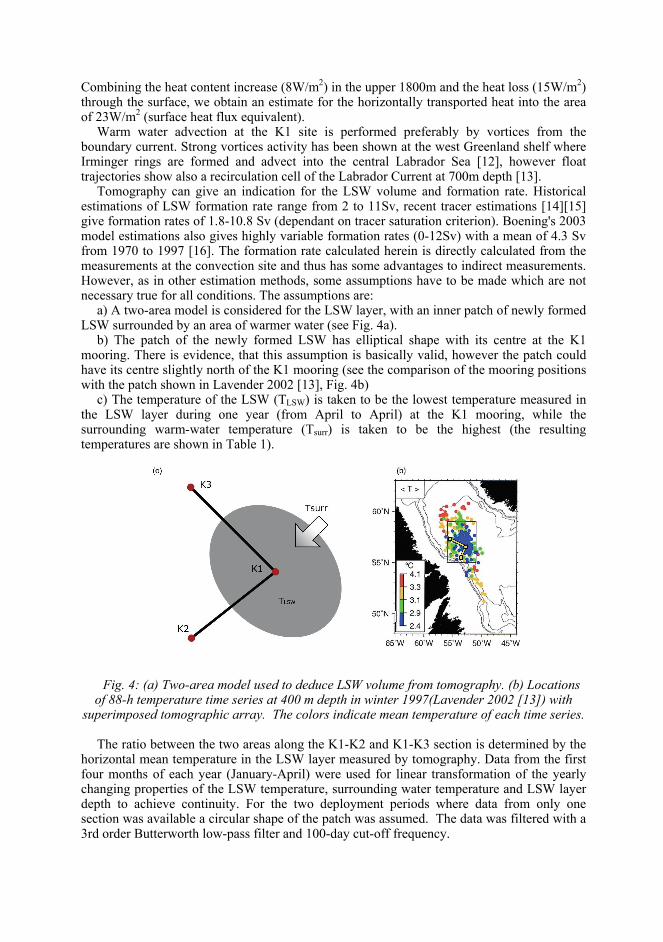
a) A two-area model is considered for the LSW layer, with an inner patch of newly formed LSW surrounded by an area of warmer water (see Fig. 4a).

b) The patch of the newly formed LSW has elliptical shape with its centre at the K1 mooring. There is evidence, that this assumption is basically valid, however the patch could have its centre slightly north of the K1 mooring (see the comparison of the mooring positions with the patch shown in Lavender 2002 [13], Fig. 4b)

c) The temperature of the LSW (TLSW) is taken to be the lowest temperature measured in the LSW layer during one year (from April to April) at the K1 mooring, while the surrounding warm-water temperature (Tsurr) is taken to be the highest (the resulting temperatures are shown in Table 1).

Fig. 4: (a) Two-area model used to deduce LSW volume from tomography. (b) Locations

of 88-h temperature time series at 400 m depth in winter 1997(Lavender 2002 [13]) with superimposed tomographic array. The colors indicate mean temperature of each time series.

The ratio between the two areas along the K1-K2 and K1-K3 section is determined by the

horizontal mean temperature in the LSW layer measured by tomography. Data from the first four months of each year (January-April) were used for linear transformation of the yearly changing properties of the LSW temperature, surrounding water temperature and LSW layer depth to achieve continuity. For the two deployment periods where data from only one section was available a circular shape of the patch was assumed. The data was filtered with a 3rd order Butterworth low-pass filter and 100-day cut-off frequency.

Fig. 5: LSW volume and formation/dissipation rate deduced from combination of

tomography data and LSW properties shown in Table 1. The upper panel in Fig. 5 shows the evolution of the LSW volume for the period 1997-

2003. In the first 5 years (1997-2002) very low LSW volumes are observed, with peaks of 1-2·1013 m3 in April. However, in the last year (2003) the volume increases remarkably to 6·1013 m3. By differentiating the volume with respect to time we obtain the formation and dissipation rate of LSW (Fig. 5 lower panel). Peak values of 2-8 Sv are observed, which are in the range of other estimations for a atmospheric state of low NAO index [16], [14], [17].

6. SUMMARY

The SFB460 project maintained a mooring array in the Central Labrador Sea from summer 1996 to summer 2003. The collected data is of various types including acoustic travel time measurements. The analysis of travel-time data was performed with the matched-peak inversion approach. The resulting horizontal mean temperature reveal a warming of 0.18°C in the upper 1800m over 5 years. Comparing this temperature to meteorological models result in lateral heat flux of 23W/m². Furthermore by applying a simple two-area model the temperature variability can be interpreted in terms of a change in the LSW volume and estimates for the corresponding formation rates were obtained.

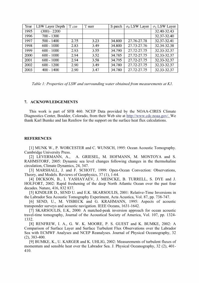
Table 1: Properties of LSW and surrounding water obtained from measurements at K1.

7. ACKNOWLEDGEMENTS

This work is part of SFB 460. NCEP Data provided by the NOAA-CIRES Climate Diagnostics Center, Boulder, Colorado, from their Web site at http://www.cdc.noaa.gov/. We thank Karl Bumke and Ian Renfrew for the support on the surface heat flux calculations.

REFERENCES

[1] MUNK W., P. WORCESTER and C. WUNSCH, 1995: Ocean Acoustic Tomography. Cambridge University Press.

[2] LEVERMANN, A., A. GRIESEL, M. HOFMANN, M. MONTOYA and S. RAHMSTORF, 2005: Dynamic sea level changes following changes in the thermohaline circulation, Climate Dynamics, 24, 347.

[3] MARSHALL, J. and F. SCHOTT, 1999: Open-Ocean Convection: Observations, Theory, and Models. Reviews of Geophysics, 37 (1), 1-64.

[4] DICKSON, B., I. YASHAYAEV, J. MEINCKE, B. TURRELL, S. DYE and J. HOLFORT, 2002: Rapid freshening of the deep North Atlantic Ocean over the past four decades. Nature, 416, 832 837.

[5] KINDLER D., SEND U. and E.K. SKARSOULIS, 2001: Relative-Time Inversions in the Labrador Sea Acoustic Tomography Experiment, Acta Acustica, Vol. 87, pp. 738-747.

[6] SEND, U., M. VISBECK and G. KRAHMANN, 1995: Aspects of acoustic transponder surveys and acoustic navigation. IEEE Oceans, 1631-1642.

[7] SKARSOULIS, E.K, 2000: A matched-peak inversion approach for ocean acoustic travel-time tomography, Journal of the Acoustical Society of America, Vol. 107, pp. 1324-1332.

[8] RENFREW, I. A., G. W. K. MOORE, P. S. GUEST and K. BUMKE, 2002: A Comparison of Surface Layer and Surface Turbulent Flux Observations over the Labrador Sea with ECMWF Analyses and NCEP Reanalyses. Journal of Physical Oceanography, 32 (2), 383-400.

[9] BUMKE, K., U. KARGER and K. UHLIG, 2002: Measurements of turbulent fluxes of momentum and sensible heat over the Labrador Sea. J. Physical Oceanography, 32 (2), 401-410.

[10] ISEMER H.J. and L. HASSE, 1987: The Bunker climate atlas of the North Atlantic Ocean: 2. Air-sea interactions, Springer, 256pp

[11] GILL, A. E. and P. P. NIILER, 1973: The theory of the seasonal variability in the ocean. Deep- See Research, 20 (2), 141-177, Part I.

[12] LILLY, J. M., P. B. RHINES, F. SCHOTT, K. L. LAVENDER, J. LAZIER, U. SEND and E. D ASARO, 2003: Observations of the Labrador Sea eddy field. Progress in Oceanography, 59, 75-176.

[13] LAVENDER, K. L., R. E. DAVIS and W. OWENS, 2002: Observations of open-ocean deep convection in the Labrador Sea from subsurface floats. Journal of Physical Oceanography, 32, 511-526.

[14] RHEIN, M., J. FISCHER, W. M. SMETHIE, D. SMYTHE-WRIGHT, R. F. WEISS, C. MERTENS, D.-H. MIN, U. FLEISCHMANN and A. PUTZKA, 2002: Labrador SeaWater: Pathways, CFC Inventory, and Formation Rates. Journal of Physical Oceanography, 32, 648-665.

[15] SMETHIE, W. M. and R. A. FINE, 2001: Rates of North Atlantic Deep Water formation calculated from chlorofluorocarbon inventories. Deep-See Research, 48, 189-215, Part I.

[16] BOENING, C. W., M. RHEIN, J. DENGG and C. DOROW, 2003: Modelling CFC inventories and formation rates of Labrador Sea Water. Geophysical Research Letters, 30 (2), 22.

[16] KHATIWALA, S., P. SCHLOSSER and M. VISBECK, 2002: Rates and Mechanisms of Water Mass Transformation in the Labrador Sea as Inferred from Tracer Observations. Journal of Physical Oceanography, 32, 666-686.