6 School of Life Sciences, University of Nottingham ...

Title: Why many Batesian mimics are inaccurate: evidence from hoverfly colour patterns 1

2

Authors: Christopher H Taylor1 3

Tom Reader1 4

Francis Gilbert1 5

1 School of Life Sciences, University of Nottingham, University Park, Nottingham, NG7 2RD 6

7

Corresponding author: Christopher Taylor 8

[email protected] 9

10

CORE Metadata, citation and similar papers at core.ac.uk

Provided by Repository@Nottingham

https://core.ac.uk/display/162662918?utm_source=pdf&utm_medium=banner&utm_campaign=pdf-decoration-v1

mailto:[email protected]

ABSTRACT 11

Mimicry is considered a classic example of the elaborate adaptations that natural selection can produce, yet 12

often similarity between Batesian (harmless) mimics and their unpalatable models is far from perfect. 13

Variation in mimetic accuracy is a puzzle, since natural selection should favour mimics that are hardest to 14

distinguish from their models. Numerous hypotheses exist to explain the persistence of inaccurate mimics, 15

but most have rarely or never been tested against empirical observations from wild populations. One reason 16

for this is the difficulty in measuring pattern similarity, a key aspect of mimicry. 17

Here, we use a recently developed method, based on the distance transform of binary images, to quantify 18

pattern similarity both within and among species for a group of hoverflies and their hymenopteran models. 19

This allowed us to test three key hypotheses regarding inaccurate mimicry. Firstly, we tested the prediction 20

that selection should be more relaxed in less accurate mimics, but found that levels of phenotypic variation 21

are similar across most hoverfly species. Secondly, we found no evidence that mimics have to compromise 22

between accuracy to multiple model species. However we did find that darker-coloured hoverflies are less 23

accurate mimics, which could lead to a trade-off between mimicry and thermoregulation in temperate 24

regions. Our results shed light on a classic problem concerning the limitations of natural selection. 25

Keywords: Batesian mimicry; imperfect mimicry; Syrphidae; distance transform; thermal melanism. 26

27

INTRODUCTION 28

Charles Darwin regarded mimicry as a beautiful example of the extreme results of natural selection [1, 29

p.392], and the topic has since been well studied as a powerful and conspicuous demonstration of the 30

evolution of phenotypes [2]. Batesian mimics are harmless organisms that resemble a more dangerous 31

“model” in order to deceive potential predators [3], and while some show an astonishing level of similarity 32

to their models, others bear only a passing resemblance. Both theory [4] and experiments [5-7] show that, in 33

practical terms, mimicry is a continuum rather than a simple binary category: inaccurate mimics are attacked 34

less frequently than non-mimics, but more often than more accurate ones [but see 8, 9]. We would 35

therefore expect the most accurate mimics in a population to have the highest fitness, and that natural 36

selection should drive ever-increasing perfection in resemblance to the model. Contrary to this prediction, 37

there are many examples, including some snakes [10], spiders [11] and hoverflies [12], that seem far from 38

accurate in their mimicry. By exploring this discrepancy between expectation and observation, the study of 39

inaccurate Batesian mimicry provides an excellent opportunity to develop a better understanding of the 40

ecological forces which determine the evolution of phenotypes. 41

There is no shortage of hypotheses proposed to address the existence of inaccurate mimicry, and these have 42

been well reviewed elsewhere [2, 13-15]. Here, we test some of the key hypotheses using hoverflies 43

(Diptera: Syrphidae) as our study organisms, but the hypotheses are equally relevant to other groups of 44

mimics. Hoverflies have been a major focus for studies of inaccurate mimicry, as the taxon comprises a large 45

number of species, many of which are abundant and widespread, ranging from non-mimetic to highly 46

accurate mimics of various hymenopteran models, with a wide range of inaccurate mimics in between [12, 47

15]. Hoverflies overlap their models extensively in space (with models such as Apis mellifera and Vespula 48

vulgaris being widespread in the Palearctic), and also in time. Most species of hoverfly first emerge between 49

March and May and remain active until at least September [16], with workers of social Hymenoptera 50

generally reaching peak abundance in July/August [17]. 51

Theoretical explanations for inaccurate Batesian mimicry have produced a number of testable predictions 52

about variation within and among mimetic species. An important group of predictions centre on the 53

cognition and behaviour of the predator, which can be modelled using Signal Detection Theory [4]. This 54

assumes that predators receive information from signals subject to noise, and therefore uncertainty. Signal 55

Detection Theory suggests that, past a certain minimum level of similarity, further improvements in mimetic 56

accuracy provide very little decrease in predation risk [18]. Mimics that have reached this critical level of 57

similarity will therefore experience relaxed selection. From this, Holloway et al. [19] make the prediction that 58

more accurate mimics should show greater phenotypic variation. They suggest that less accurate mimics are 59

under strong selection but lack the genetic variation to evolve closer similarity to the model, and hence have 60

low phenotypic variation. 61

However, alternative predictions arise if we consider that mimic species may not all be equally attractive to 62

predators. The threshold similarity level described above, beyond which selection is relaxed [18], depends on 63

what has been described as the “incentive to attack” [20]. A predator is less likely to risk an attack with an 64

uncertain outcome if the cost of attacking a model is high relative to the benefit of consuming a mimic, or if 65

the abundance of models is high relative to the mimics. One possible cause of low incentive to attack is given 66

by Penney et al. [21], who argue that smaller mimics have a lower calorific value to the predator, resulting in 67

a low incentive to attack, and hence favouring relatively imperfect mimicry in smaller species. Regardless of 68

the exact reasons behind the costs and benefits to a predator, if a certain group of mimics offer a low 69

incentive to attack, they are predicted to be under relatively relaxed selection by predators compared with 70

other species, and may therefore show greater phenotypic variability. 71

We must also consider that predators may be influenced by more than one model phenotype. Mathematical 72

models predict that mimics with an intermediate similarity to several model species can be better protected 73

than an accurate mimic of a single model species [14, 18], and thus increasing similarity to one model might 74

come at the cost of lower accuracy to another. It is highly likely that predators will encounter more than one 75

model species in their foraging, but the extent to which this influences inaccurate mimicry is not known [14, 76

15]. 77

Finally, if selective pressures other than those imposed by predators influence the mimic’s appearance, then 78

inaccurate mimics could represent a trade-off between such opposing pressures. For example, increasing 79

similarity to the model may come with a physiological cost, such as reduced ability to regulate temperature. 80

Hoverfly colour patterns are known to vary with temperature both seasonally and geographically [22], and 81

this variation is thought to confer a survival advantage in response to differing thermoregulatory constraints 82

[23]. In temperate climates, darker coloured insects are able to warm up more quickly [24, 25], and thus 83

improve performance in areas such as flight activity [26]. It is highly plausible that such a mechanism 84

underlies colour variation in hoverflies. However, to our knowledge, the effect of this variation on mimetic 85

accuracy has never been assessed. We would expect to see a conflict in temperate regions between the 86

bright colours required for mimicry and dark colours that allow effective temperature regulation. 87

Among the wealth of theories which seek to explain inaccurate mimicry, most have been studied through 88

mathematical modelling or abstract experiments [2, 13]. Only recently has attention turned to a broader 89

perspective of testing the various hypotheses against each other in real systems, which is the only way in 90

which the relative merits of the different hypotheses can be accurately assessed. Penney et al. [21] carried 91

out a comparative study of 38 hoverfly species, along with 10 putative models, using both morphological 92

data and human judgment to measure degree of similarity. They found evidence that inaccurate mimics are 93

not just artefacts of human perception, and suggested that no species are intermediate between several 94

models. However, they found a positive relationship between size and mimetic accuracy, which they 95

interpret as evidence for the relaxed selection theory, suggesting that larger hoverflies are more valuable 96

prey and therefore under stronger selective pressure. 97

Another comparative study by Holloway et al. [19] investigated the levels of phenotypic variation in a 98

number of hoverfly and wasp species. They used rankings of mimetic accuracy as calculated from 99

behavioural responses of pigeons recorded in Dittrich et al. [6], and were consequently limited to the few 100

species used in the pigeon study. Holloway et al. [19] found high levels of variation in many species, giving no 101

indication that a lack of genetic variation was limiting the evolution of accuracy. They did not find a clear 102

trend between mimetic accuracy and phenotypic variation, although particularly high variation in the model 103

species and one accurate mimic, Temnostoma vespiforme, led them to conclude that relaxed selection may 104

be acting in those cases. 105

The few empirical studies which have attempted to test predictions about variation in mimetic accuracy have 106

been constrained by the difficulties of generating effective measures of similarity between mimics and their 107

models. It is possible to use predator behaviour to rank similarity [e.g. 6], but this approach becomes 108

prohibitively expensive if applied to large numbers of specimens, and so in large-scale studies, a 109

mathematical similarity measure is essential. For example, Holloway et al. [19] characterized mimic 110

phenotype simply using the proportion of yellow versus black on two tergites of the abdomen. The 111

descriptors that Penney et al. [21] used to create a multivariate measure of mimetic accuracy included 112

morphometric data (e.g. antenna length, thorax width, wing length) as well as some summary variables 113

relating to the abdominal pattern (e.g. mean red-green-blue values, number of stripes), but very little about 114

the pattern itself. 115

Recently, we have developed a new objective measure of mimetic accuracy by comparing entire abdominal 116

patterns using the distance transform method [27]. This method is not intended as a faithful representation 117

of a potential predator’s cognitive processes, which in any case are not currently known, but as an objective 118

means of capturing detailed information about pattern variation, beyond simple summary measures such as 119

colour proportions. Nonetheless, our method provides a measure of mimetic accuracy much closer to 120

human and avian estimates than previous empirical measures, even without the inclusion of any 121

morphometric data [27]. In the current study, we use this new methodology to characterize the mimetic 122

patterns of hoverflies in detail, and to test some of the predictions which have emerged from theoretical 123

work. We plot a large number of model and mimic individuals in “similarity space”, giving a picture not only 124

of how species compare with one another in appearance, but also of the variation within species. We then 125

test four predictions associated with three theoretical explanations for the existence of inaccurate mimicry: 126

1. Relaxed selection 127

a. Lack of genetic variation: Less accurate mimics are under strong selection but lack the 128

genetic variation to evolve increased accuracy; more accurate mimic species experience 129

relaxed selection and thus have higher levels of phenotypic variation. 130

b. Incentive to attack: Less accurate mimic species have higher levels of phenotypic variation 131

since they provide a lower incentive to attack and are under more relaxed selection. 132

2. Multiple models: Increasing accuracy to one model decreases accuracy to others; inaccurate mimics 133

represent a compromise between two or more model phenotypes. 134

3. Thermoregulation: Less accurate mimics have more black in their pattern and hence will be better 135

able to regulate their temperature; there is a trade-off between accurate mimicry and effective 136

thermoregulation. 137

138

METHODS 139

Image processing and dissimilarity calculations were carried out in MATLAB [28]. Statistical analyses were 140

carried out in R version 3.0.3 [29]. 141

Specimens 142

Insects were collected using a hand net from wild communities in Nottinghamshire, UK (particularly the 143

Attenborough Nature Reserve) and surrounding areas, during May to October in the years 2012-2014. See 144

Table S1 for full details of sampling sites. Target insects were any hoverflies or stinging Hymenoptera bearing 145

a two-colour pattern (usually black and yellow; see example images in Figure S1), but excluding bumblebees 146

and their putative mimics, which are notably much hairier than other the other taxa encountered (making 147

automated characterization of the abdominal pattern difficult), and which are very likely part of a different 148

mimicry ring [15]. We follow other studies such as [21] in excluding male Hymenoptera from the analysis as, 149

not having a sting, their status as models is debatable (they may still be unpalatable to predators due to 150

other factors [5]). Males are also of much lower abundance than females for most of the year, and thus only 151

five specimens were excluded from this study. A total of 954 individuals were identified to species level and 152

sexed using relevant keys [16, 17, 30]. 153

Specimens were euthanised by freezing, and their legs and wings pinned out to the sides when necessary to 154

give a clear view of the abdomen. They were then placed inside a homemade “photo studio” – a white 30 x 155

18 x 10 cm open topped box. A 5mm scale bar was placed near to the insect. Specimens were photographed 156

from above with a Canon 600D DSLR camera and Tamron 90mm macro lens under natural outdoor light 157

conditions, in the shade. This method resulted in images that were evenly lit and free from strong reflections 158

or glare. While natural weather variation did lead to some changes in brightness from image to image, this 159

did not affect the analysis since patterns were converted to binary form before comparison (see “image 160

processing”). 161

Image processing 162

Images were rotated, cropped, and rescaled to a standard alignment, and an algorithm was applied to 163

remove noise and sharpen edges. An edge detection algorithm was used to find the outline of the abdomen. 164

In some cases, a rough outline was drawn manually and passed to the algorithm as a starting point, to fix 165

cases where the outline was difficult to detect against the background. 166

The abdomen was automatically segmented into two colour regions (typically black and yellow/orange). 167

Some images (129 out of 954) did not produce clear segmentations, often due to fading of the colours after 168

death (C. Taylor 2012, pers. obs.) and were discarded from further analyses. To quantify the colour 169

proportions in the pattern, we calculated the proportion of pixels within the abdominal image that were 170

classified as “black” (i.e. the darker of the two segments) after segmentation. 171

See SI Text and Figure S2 for more detail on the image processing. 172

Mimetic accuracy 173

We calculated dissimilarity values for all possible pairings of images within the dataset using the distance 174

transform method [27]. Optimization of the method used translation and scaling in the vertical direction to 175

account for any slight misalignment of the patterns. For some subsequent figures and analyses, it is more 176

intuitive to work with measures of mimetic accuracy than with dissimilarity. To make the conversion, we 177

used the formula A = 1 – (D / Dmax), where A is mimetic accuracy, D is dissimilarity and Dmax is the largest 178

dissimilarity value between any two individuals in the overall dataset. This scales mimetic accuracy to run 179

from a minimum of 0 (defined by this particular dataset) to a maximum of 1 (independent of the dataset – 180

identical images). For each individual mimic, we calculated the mean similarity with respect to all individuals 181

of a given model species, to give a measure of mimetic accuracy to that model. 182

We first tested for sexual dimorphism in the hoverfly species, since males and females may have different 183

levels of mimetic accuracy, or might even resemble different models. For example, it has been suggested 184

that female Eristalis arbustorum are bee mimics, while the males mimic wasps [31]. For each mimic species 185

in our dataset for which we have data on at least three males and three females, we tested for dimorphism 186

in both size and pattern. For size, we carried out a Wilcoxon two-sample test on thorax width data. For 187

pattern, we used distance-based multivariate analysis [32, 33] carried out in the program DISTLM5. This 188

allows the equivalent of ANOVA to be carried out directly on distance (dissimilarity) data rather than having 189

to ordinate the data first. Species were considered dimorphic if p < 0.05 for either of the above tests, in 190

which case the sexes were treated separately in all subsequent analyses. For species where p > 0.05 for both 191

size and pattern, and those with fewer than three individuals in one or other sex, data from males and 192

females were pooled in subsequent analyses. We refer to these groupings as “Species or Sex Units”, or SSUs. 193

The mimetic accuracy for an SSU was calculated as the mean of the individual values of mimetic accuracy 194

within that SSU, again for each model species separately. We then assigned each SSU a “best” model, being 195

the potential model for which it has the highest mean accuracy value. Four species of Hymenoptera were 196

treated as the candidate models of the sampled community (Figure S1), being the only potential models that 197

were common in our samples (N > 3): Vespula vulgaris (common wasp), Vespula germanica (German wasp), 198

Vespa crabro (hornet) and Apis mellifera (honeybee). We know from both theory [34] and experiments [35] 199

that a model’s importance in shaping predator behaviour increases with its abundance, and therefore we 200

have excluded eight low-abundance (N ≤ 3) model species from the main analysis. However, we did also 201

repeat our analysis including these rarer model species (see SI Text). 202


To quantify variation within SSUs, we first ordinated the dissimilarity data by using Principal Coordinates 204

Analysis (PCoA) [36]. We chose this method of ordination, as opposed to non-metric multidimensional 205

scaling, as we considered it important to use a method in which the resulting inter-point distances would be 206

linearly related to the original distance matrix. We did this in order to preserve the magnitude of the 207

variation in the dataset, despite the fact that PCoA assumes that distances between individuals are metric 208

(that is, they obey the triangle inequality), which is not always the case when using distances generated by 209

the distance transform method [27]. 210

On the basis of a scree plot, we chose the first four dimensions of the PCoA as the best representation of the 211

data. Using these four dimensions, we calculated the centroid for each SSU, and then the distance, z, of each 212

individual to its corresponding centroid. The mean of a group’s z values provides a measure of within-group 213

variability [33]. 214

When testing the relationship between mimetic accuracy and within-taxon variability in accuracy, using raw 215

similarity values as a measure of mimetic accuracy is not appropriate. If a model and mimic species overlap 216

in phenotypic space, we risk creating a circular argument. Mimics that are more variable will inevitably show 217

lower accuracy, since a greater spread in phenotypic space will lead to larger distances (on average) to the 218

model phenotype. For this test, therefore, we used a different measure of mimetic accuracy that is not 219

affected by the phenotypic variability. After ordination using PCoA, we calculated centroid points for mimic 220

and model species and defined (in)accuracy as the distance from a mimic’s centroid to the closest model 221

centroid. 222

To test for an influence of mimetic accuracy on within-taxon variability, we ran a generalized least squares 223

model (GLS) [37] in the R package “ape” version 3.1-1 [38]. GLS is equivalent to a general linear model, but 224

with the inclusion of a correlation matrix derived from the species’ phylogeny to control for relatedness 225

among species. We used mean z value for an SSU as the response and mean mimetic accuracy and mean 226

thorax width (plus their interaction) as predictors. Thorax width was included in the model as a proxy for size 227

[39], because Penney et al. [21] argued that larger hoverflies should offer a larger “incentive to attack” due 228

to their greater nutritional value. The width of the thorax at the base of the wings was measured in ImageJ 229

[40] using the unprocessed images, using a 5 mm bar in each image to set the scale. Note that in the early 230

stages of the project, photographs did not include a scale bar, and therefore in some cases (e.g. see Table S2) 231

samples for size measurements are smaller than for other measures such as pattern. 232

We tested the model under two different evolutionary scenarios: Brownian motion (BM) evolution, and 233

Ornstein-Uhlenbeck (OU) evolution (similar to BM, but traits are constrained towards an “optimum” value). 234

These different scenarios were represented by two different correlation matrices passed to the GLS model, 235

calculated from a composite phylogeny (Figure S3) based on information from Rotheray and Gilbert [41] and 236

Ståhls et al. [42]. For both females and males, the OU evolutionary model was found to be a significantly 237

better fit to the data (females: Likelihood Ratio (LR) = 11.71, p = 0.0006; males: LR = 6.10, p = 0.014; both df 238

= 1) and was used for subsequent analysis. We then used backwards stepwise model simplification with 239

likelihood ratio tests to find the minimum adequate model. In order to allow for sexual dimorphism, we 240

conducted two separate analyses, one with data from only female individuals, and the other with only 241

males. 242

2. Multiple models 243

To test for a potential trade-off in similarity to multiple models, we tested within SSUs for correlation (using 244

Pearson’s r) in mimetic accuracy towards the four main model species. A negative correlation would imply 245

that, for a given SSU, increasing similarity to one model comes at the cost of decreased similarity to another. 246

We tested all SSUs for which we had data on at least six individuals. 247

3. Thermoregulation 248

We tested for a trade-off between accuracy and the extent of black in the pattern (“proportion black”) using 249

a Markov Chain Monte Carlo generalised linear mixed model, implemented in the R package “MCMCglmm” 250

[43]. Again, this method allowed us to control for phylogenetic relatedness among species. Accuracy of 251

individual mimics to their closest model was the response variable, logit transformed for normality of 252

residuals. Fixed effects were the proportion black, thorax width, sex and season, along with all two-way 253

interactions. Thorax width was included as a proxy for size (see above), which can have a major impact on 254

thermoregulation [44]. Season was included because selection on thermoregulation may vary according to 255

the time of year. We categorised season as “early” (to 8th August) or “late” (9th August onwards) splitting at 256

the date of the median sample, which also fell roughly halfway between the first and last sampling days. We 257

also conducted a more complex analysis in which time of year was treated as a continuous variable, 258

including a quadratic term, which gave very similar results. Species was included as a random effect, and we 259

calculated a covariance structure for the random effect based on the phylogenetic tree (Figure S3; also see 260

“relaxed selection” above). We used backwards stepwise model simplification based on p values to find the 261

minimum adequate model. Note that in Figure 2, proportion black and thorax width are binned for ease of 262

interpretation, but they were treated as continuous in the analysis. 263

264

RESULTS 265

We examined pattern similarity among 697 hoverfly (54 species) and 128 hymenopteran individuals (12 266

species). We found evidence for size dimorphism in seven of the mimic species in our dataset, and for 267

pattern dimorphism in a further eleven (Table S2), giving a total of 72 SSUs. Compared against the four most 268

abundant species of Hymenoptera from our samples, 51 SSUs were classed as mimics of Vespula vulgaris, 11 269

of Apis mellifera, seven of Vespa crabro, and three of Vespula germanica. The level of mimetic accuracy to 270

the assigned model varied from 0.55 to 0.87 (Table S3, Figure S4). 271


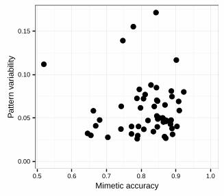
If inaccurate mimics have insufficient genetic variation to reach a level of protection at which selection 273

becomes relaxed, we predict a positive correlation between pattern variability within species and similarity 274

to the model. Alternatively, if less accurate mimic species provide a low incentive for predators to attack, for 275

example because of a low calorific value, we predict a negative correlation. However, after controlling for 276

shared ancestry, phenotypic variability was not significantly associated with either mimetic accuracy or body 277

size (thorax width) in either males or females (Table 1 and Figure 1; see also Table S4). 278

2. Multiple models 279

If mimetic accuracy is limited by a trade-off among similarities to several models, we predict that similarity 280

to different model species should be negatively correlated. However, almost all SSUs show either a 281

significant positive correlation or no significant correlation among similarity values to the four main model 282

species (Table S5). There was only one negative correlation with p < 0.05: in males of Syrphus ribesii, 283

accuracy to Apis mellifera was negatively correlated with accuracy to Vespa crabro (r = -0.56, p = 0.009, N = 284

21). Under the null hypothesis, if all tests were independent, we would expect 10 negative correlations 285

through type I error on average. 286

3. Thermoregulation 287

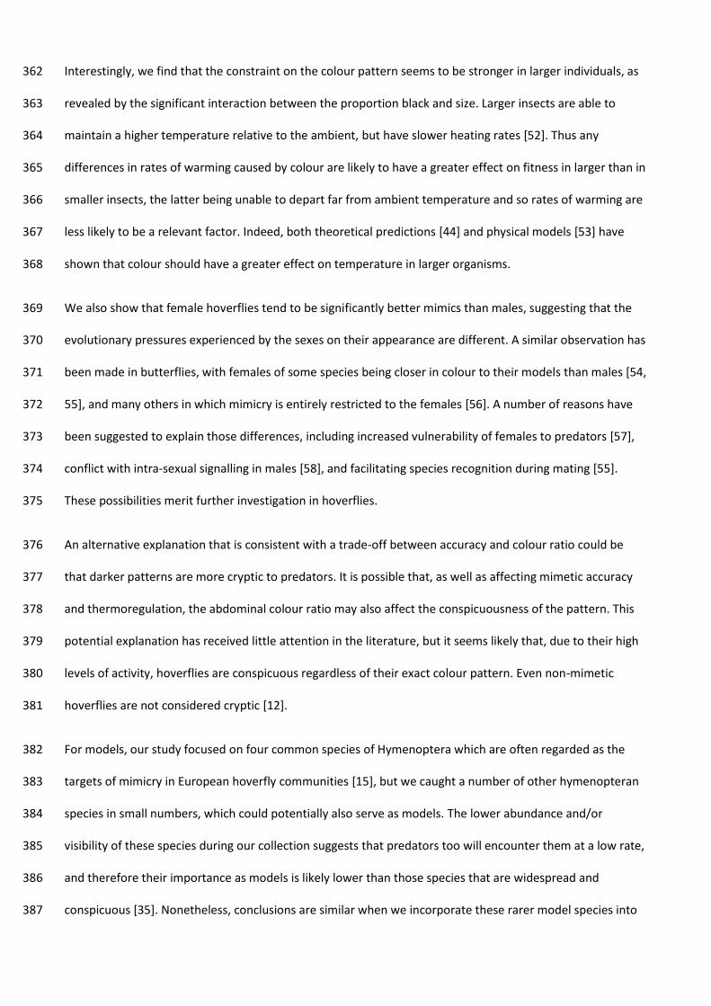
If mimetic accuracy is limited by a trade-off with thermoregulation, we predict a negative correlation 288

between similarity to the model and the proportion of the pattern that is black. Having controlled for shared 289

ancestry, there is a significant negative interaction between proportion black and thorax width (p = 0.040; 290

Table 2). When combined with the other estimated coefficients (Table 2) this indicates that those mimics 291

with a greater proportion of black on their abdomen tend to be less accurate to their model, and that this 292

trend is particularly strong in larger mimics (Figure 2). There is a significant effect of sex, with females in 293

general being more accurate (p < 0.001). In addition, both proportion black (p < 0.001) and thorax width (p < 294

0.001) interact with sex, with females showing a weaker version of the trend described above. These trends 295

observed in colour, size and sex are evident even having accounted for seasonal differences in mimetic 296

accuracy (Table 2 and Figure 2; see also Tables S6-7 and Figure S5). 297

298

DISCUSSION 299

By comparing colour patterns using the distance transform method [27] we have been able to quantify in 300

detail the mimetic relationships in a community of insects, including variation both within and among 301

species. The lack of a trend between accuracy and phenotypic variation suggests that inaccurate mimics are 302

not accounted for by the fact that they have not been able to evolve to the point of maximum protection 303

(Prediction 1a) or by relaxed selection caused by a reduced incentive of predators to attack (Prediction 1b). 304

Rather, the data suggest that inaccurate phenotypes represent the result of a trade-off between opposing 305

selective pressures. A trade-off caused by selection for similarity to multiple models (Prediction 2) is not 306

supported, but the results point towards a hitherto unexplored role for thermoregulation in limiting the 307

adaptive value of increased accuracy (Prediction 3). 308

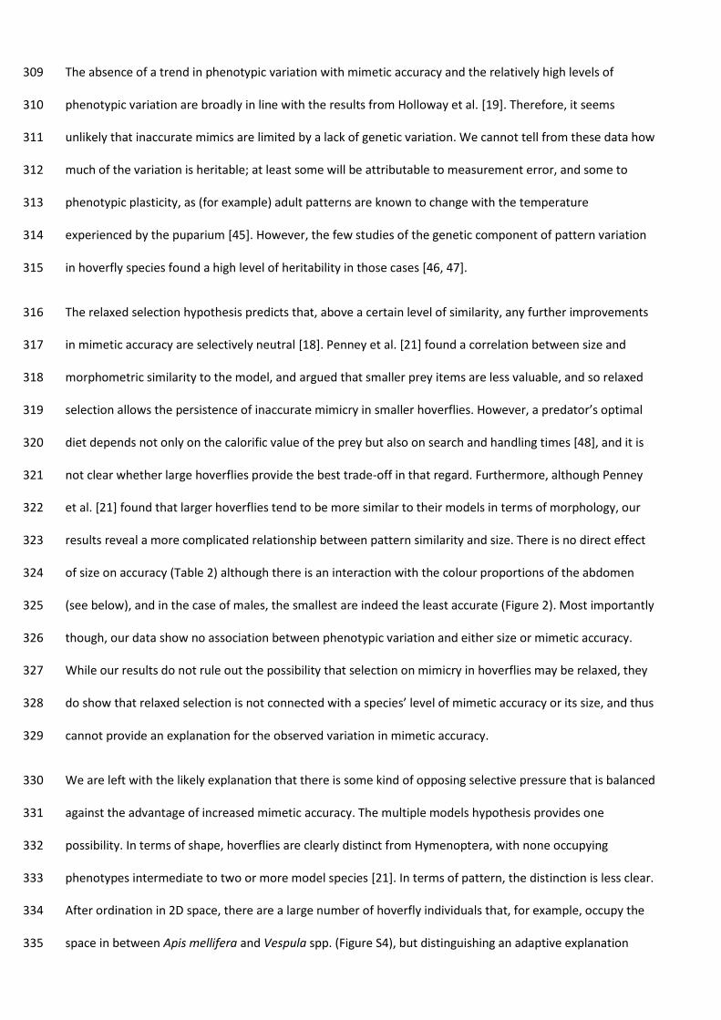
The absence of a trend in phenotypic variation with mimetic accuracy and the relatively high levels of 309

phenotypic variation are broadly in line with the results from Holloway et al. [19]. Therefore, it seems 310

unlikely that inaccurate mimics are limited by a lack of genetic variation. We cannot tell from these data how 311

much of the variation is heritable; at least some will be attributable to measurement error, and some to 312

phenotypic plasticity, as (for example) adult patterns are known to change with the temperature 313

experienced by the puparium [45]. However, the few studies of the genetic component of pattern variation 314

in hoverfly species found a high level of heritability in those cases [46, 47]. 315

The relaxed selection hypothesis predicts that, above a certain level of similarity, any further improvements 316

in mimetic accuracy are selectively neutral [18]. Penney et al. [21] found a correlation between size and 317

morphometric similarity to the model, and argued that smaller prey items are less valuable, and so relaxed 318

selection allows the persistence of inaccurate mimicry in smaller hoverflies. However, a predator’s optimal 319

diet depends not only on the calorific value of the prey but also on search and handling times [48], and it is 320

not clear whether large hoverflies provide the best trade-off in that regard. Furthermore, although Penney 321

et al. [21] found that larger hoverflies tend to be more similar to their models in terms of morphology, our 322

results reveal a more complicated relationship between pattern similarity and size. There is no direct effect 323

of size on accuracy (Table 2) although there is an interaction with the colour proportions of the abdomen 324

(see below), and in the case of males, the smallest are indeed the least accurate (Figure 2). Most importantly 325

though, our data show no association between phenotypic variation and either size or mimetic accuracy. 326

While our results do not rule out the possibility that selection on mimicry in hoverflies may be relaxed, they 327

do show that relaxed selection is not connected with a species’ level of mimetic accuracy or its size, and thus 328

cannot provide an explanation for the observed variation in mimetic accuracy. 329

We are left with the likely explanation that there is some kind of opposing selective pressure that is balanced 330

against the advantage of increased mimetic accuracy. The multiple models hypothesis provides one 331

possibility. In terms of shape, hoverflies are clearly distinct from Hymenoptera, with none occupying 332

phenotypes intermediate to two or more model species [21]. In terms of pattern, the distinction is less clear. 333

After ordination in 2D space, there are a large number of hoverfly individuals that, for example, occupy the 334

space in between Apis mellifera and Vespula spp. (Figure S4), but distinguishing an adaptive explanation 335

from random placement is difficult. Crucially, for each species of mimic, there is either no correlation or a 336

positive correlation among similarity values to each potential model species. This implies that, at least in 337

terms of pattern, there is no multi-model trade-off: assuming the observed variation has an underlying 338

genetic component, it would be possible for each mimic to improve its similarity to one or more models 339

without compromising similarity to others. We cannot rule out multiple models having an influence on the 340

phenotype of a mimic, but we can conclude that the multiple models hypothesis is not sufficient to explain 341

the observed levels of inaccuracy. 342

In contrast, a trade-off between mimicry and thermoregulation is consistent with our data. Hoverflies 343

maintain a temperature excess (a body temperature above that of the surrounding air) through a 344

combination of basking and shivering [49]. Darker coloured insects absorb more solar radiation, and 345

therefore can heat up more rapidly [24, 25], so we expect darker hoverflies to be at a fitness advantage in 346

cooler conditions. More rapid temperature gain during basking will reduce the opportunity cost of 347

thermoregulation as well as possibly reducing predation risk. In support of this, a number of hoverfly species 348

have been found to show seasonal variation in their colour patterns, with darker morphs being more 349

common outside the summer months [45], which is thought to have an adaptive function in relation to 350

temperature regulation [23]. 351

However, the results of our study show that the thermoregulatory benefits of darker patterns will also likely 352

be associated with a reduction in mimetic accuracy. To be a perfect mimic of Vespula vulgaris, the most 353

abundant model in our samples, would require the amount of black on the abdomen to be limited to 51%, 354

but almost all hoverflies surveyed were above this value (Table S3). Aposematic signals are known to 355

constrain temperature regulation, as observed in the moth Parasemia plantagenis [50]. Moths with more 356

black on their body were able to warm up more quickly, but suffered increased predation due to a less 357

effective warning signal. Thus it is highly plausible that hoverfly colour patterns are constrained by their 358

thermoregulation function. By contrast, wasp abdominal patterns are likely to be less constrained, since they 359

do not rely much on basking for thermoregulation; social wasps achieve a high temperature excess through 360

endothermy before they even leave their nest [51]. 361

Interestingly, we find that the constraint on the colour pattern seems to be stronger in larger individuals, as 362

revealed by the significant interaction between the proportion black and size. Larger insects are able to 363

maintain a higher temperature relative to the ambient, but have slower heating rates [52]. Thus any 364

differences in rates of warming caused by colour are likely to have a greater effect on fitness in larger than in 365

smaller insects, the latter being unable to depart far from ambient temperature and so rates of warming are 366

less likely to be a relevant factor. Indeed, both theoretical predictions [44] and physical models [53] have 367

shown that colour should have a greater effect on temperature in larger organisms. 368

We also show that female hoverflies tend to be significantly better mimics than males, suggesting that the 369

evolutionary pressures experienced by the sexes on their appearance are different. A similar observation has 370

been made in butterflies, with females of some species being closer in colour to their models than males [54, 371

55], and many others in which mimicry is entirely restricted to the females [56]. A number of reasons have 372

been suggested to explain those differences, including increased vulnerability of females to predators [57], 373

conflict with intra-sexual signalling in males [58], and facilitating species recognition during mating [55]. 374

These possibilities merit further investigation in hoverflies. 375

An alternative explanation that is consistent with a trade-off between accuracy and colour ratio could be 376

that darker patterns are more cryptic to predators. It is possible that, as well as affecting mimetic accuracy 377

and thermoregulation, the abdominal colour ratio may also affect the conspicuousness of the pattern. This 378

potential explanation has received little attention in the literature, but it seems likely that, due to their high 379

levels of activity, hoverflies are conspicuous regardless of their exact colour pattern. Even non-mimetic 380

hoverflies are not considered cryptic [12]. 381

For models, our study focused on four common species of Hymenoptera which are often regarded as the 382

targets of mimicry in European hoverfly communities [15], but we caught a number of other hymenopteran 383

species in small numbers, which could potentially also serve as models. The lower abundance and/or 384

visibility of these species during our collection suggests that predators too will encounter them at a low rate, 385

and therefore their importance as models is likely lower than those species that are widespread and 386

conspicuous [35]. Nonetheless, conclusions are similar when we incorporate these rarer model species into 387

the analysis (see SI Text). We also note that the four common model species from our study all increase in 388

abundance during late summer/early autumn, and that this change could potentially affect the dynamics of 389

the mimetic community. However, the relationship between colour and mimetic accuracy cannot be 390

explained by seasonal effects, since it was observed even after seasonal variation was taken into account. 391

The phenotypic correlations we have described are consistent with a trade-off between mimicry and 392

thermoregulation, but we acknowledge that, due to the comparative nature of this study, we have not been 393

able to test this trade-off directly. As we have discussed, the mechanisms that we suggest may be 394

responsible for the observed correlation are consistent with what is known about mechanisms of insect 395

thermoregulation. Further work is now needed to test the effects of colour variation on both predation and 396

temperature of hoverflies in an experimental setting. Comparison of mimetic communities from different 397

climates may also provide a fruitful means of examining the conflict between mimicry and thermoregulation 398

in more detail. 399

Ethics 400

Collection of insect specimens was approved by the Nottinghamshire Wildlife Trust. 401

Data accessibility 402

The original dataset on which our analyses were based is available in Table S8. 403

Competing interests 404

We have no competing interests. 405

Authors’ contributions 406

CT collected and analysed data and wrote the first draft of the manuscript. CT, TR and FG conceived the 407

study and revised the manuscript. All authors gave final approval for publication. 408

Acknowledgements 409

We thank staff at the Attenborough Nature Reserve and Nottinghamshire Wildlife Trust for permission to 410

collect specimens, and Chris du Feu and Katie Threadgill for assistance with fieldwork. We thank several 411

anonymous referees for their insightful comments on previous versions of the manuscript. 412

Funding 413

This study received no external funding. 414

415

REFERENCES 416

[1] Darwin, F. 1887 The Life and Letters of Charles Darwin, vol. 2. London, UK, John Murray. 417

[2] Ruxton, G.D., Sherratt, T.N. & Speed, M.P. 2004 Avoiding Attack: The Evolutionary Ecology of Crypsis, 418

Warning Signals, and Mimicry. Oxford, Oxford University Press. 419

[3] Bates, H.W. 1862 XXXII. Contributions to an Insect Fauna of the Amazon Valley. Lepidoptera: Heliconidæ. 420

Trans. Linn. Soc. Lond. 23, 495-566. (doi:10.1111/j.1096-3642.1860.tb00146.x). 421

[4] Oaten, A., Pearce, C.E.M. & Smyth, M.E.B. 1975 Batesian mimicry and signal detection theory. Bull. Math. 422

Biol. 37, 367-387. 423

[5] Mostler, G. 1935 Beobachtungen zur frage der wespenmimikry [Observations on the question of wasp 424

mimicry]. Zoomorphology 29, 381-454. (doi:10.1007/bf00403719). 425

[6] Dittrich, W., Gilbert, F., Green, P., Mcgregor, P. & Grewcock, D. 1993 Imperfect mimicry: a pigeon's 426

perspective. Proc. R. Soc. Lond. B 251, 195-200. 427

[7] Mappes, J. & Alatalo, R.V. 1997 Batesian mimicry and signal accuracy. Evolution 51, 2050-2053. 428

[8] Valkonen, J.K., Nokelainen, O. & Mappes, J. 2011 Antipredatory function of head shape for vipers and 429

their mimics. PLoS ONE 6, e22272. (doi:10.1371/journal.pone.0022272). 430

[9] Hossie, T.J. & Sherratt, T.N. 2013 Defensive posture and eyespots deter avian predators from attacking 431

caterpillar models. Anim. Behav. 86, 383-389. (doi:http://dx.doi.org/10.1016/j.anbehav.2013.05.029). 432

[10] Greene, H.W. & McDiarmid, R.W. 1981 Coral snake mimicry: does it occur? Science 213, 1207-1212. 433

[11] Pekár, S. & Jarab, M. 2011 Assessment of color and behavioral resemblance to models by inaccurate 434

myrmecomorphic spiders (Araneae). Invertebr. Biol. 130, 83-90. 435

[12] Rotheray, G.F. & Gilbert, F. 2011 The Natural History of Hoverflies. Cardigan, UK, Forrest Text. 436

[13] Kikuchi, D.W. & Pfennig, D.W. 2013 Imperfect mimicry and the limits of natural selection. Q. Rev. Biol. 437

88, 297-315. (doi:10.1086/673758). 438

[14] Edmunds, M. 2000 Why are there good and poor mimics? Biol. J. Linn. Soc. 70, 459-466. 439

(doi:10.1111/j.1095-8312.2000.tb01234.x). 440

[15] Gilbert, F. 2005 The evolution of imperfect mimicry. In Insect Evolutionary Ecology (eds. M. Fellowes, G. 441

Holloway & J. Rolff), pp. 231-288. Wallingford, UK, CABI. 442

[16] Stubbs, A.E. & Falk, S.J. 2002 British Hoverflies: An Illustrated Identification Guide. Reading, UK, British 443

Entomological and Natural History Society. 444

[17] Richards, O.W. 1980 Scolioidea, Vespoidea and Sphecoidea; Hymenoptera, Aculeata. London, UK, Royal 445

Entomological Society of London. 446

[18] Sherratt, T.N. 2002 The evolution of imperfect mimicry. Behav. Ecol. 13, 821-826. 447

[19] Holloway, G., Gilbert, F. & Brandt, A. 2002 The relationship between mimetic imperfection and 448

phenotypic variation in insect colour patterns. Proc. R. Soc. Lond. B 269, 411-416. 449

[20] Johnstone, R.A. 2002 The evolution of inaccurate mimics. Nature 418, 524-526. 450

[21] Penney, H.D., Hassall, C., Skevington, J.H., Abbott, K.R. & Sherratt, T.N. 2012 A comparative analysis of 451

the evolution of imperfect mimicry. Nature 483, 461-464. 452

(doi:http://www.nature.com/nature/journal/v483/n7390/abs/nature10961.html#supplementary-453

information). 454

[22] Holloway, G.J. 1993 Phenotypic variation in colour pattern and seasonal plasticity in Eristalis hoverflies 455

(Diptera: Syrphidae). Ecol. Entomol. 18, 209-217. 456

[23] Ottenheim, M.M., Wertheim, B., Holloway, G.J. & Brakefield, P.M. 1999 Survival of colour polymorphic 457

Eristalis arbustorum hoverflies in semi field conditions. Funct. Ecol. 13, 72-77. 458

[24] Kingsolver, J.G. 1987 Evolution and coadaptation of thermoregulatory behavior and wing pigmentation 459

pattern in pierid butterflies. Evolution 41, 472-490. (doi:10.2307/2409250). 460

[25] Willmer, P.G. & Unwin, D.M. 1981 Field analyses of insect heat budgets: Reflectance, size and heating 461

rates. Oecologia 50, 250-255. (doi:10.1007/BF00348047). 462

[26] Ellers, J. & Boggs, C.L. 2004 Functional ecological implications of intraspecific differences in wing 463

melanization in Colias butterflies. Biol. J. Linn. Soc. 82, 79-87. (doi:10.1111/j.1095-8312.2004.00319.x). 464

[27] Taylor, C.H., Gilbert, F. & Reader, T. 2013 Distance transform: a tool for the study of animal colour 465

patterns. Methods Ecol. Evol. 4, 771-781. (doi:10.1111/2041-210x.12063). 466

[28] MATLAB. 2012 MATLAB. (Natick, Massachusetts, The Mathworks. 467

[29] R Core Team. 2014 R: A language and environment for statistical computing. (Vienna, Austria, R 468

Foundation for Statistical Computing. 469

[30] Perkins, R.C.L. 1919 The British species of Andrena and Nomada. Transactions of the Entomological 470

Society of London 1919, 218-319. 471

[31] Heal, J.R. 1981 Colour patterns of Syrphidae. III. Sexual dimorphism in Eristalis arbustorum. Ecol. 472

Entomol. 6, 119-127. (doi:10.1111/j.1365-2311.1981.tb00600.x). 473

[32] Anderson, M.J. 2001 A new method for non-parametric multivariate analysis of variance. Austral Ecol. 474

26, 32-46. (doi:10.1111/j.1442-9993.2001.01070.pp.x). 475

[33] McArdle, B.H. & Anderson, M.J. 2001 Fitting multivariate models to community data: a comment on 476

distance-based redundancy analysis. Ecology 82, 290-297. (doi:10.1890/0012-477

9658(2001)082[0290:fmmtcd]2.0.co;2). 478

[34] Getty, T. 1985 Discriminability and the sigmoid functional response: how optimal foragers could stabilize 479

model-mimic complexes. Am. Nat. 125, 239-256. 480

[35] Lindström, L., Alatalo, R.V. & Mappes, J. 1997 Imperfect Batesian mimicry—the effects of the frequency 481

and the distastefulness of the model. Proc. R. Soc. Lond. B 264, 149-153. 482

[36] Legendre, P. & Legendre, L. 1998 Numerical Ecology. 2nd English ed. ed. Amsterdam, Elsevier. 483

[37] Grafen, A. 1989 The phylogenetic regression. Philosophical Transactions of the Royal Society B: 484

Biological Sciences 326, 119-157. (doi:10.2307/2396904). 485

[38] Paradis, E., Claude, J. & Strimmer, K. 2004 APE: Analysis of Phylogenetics and Evolution in R language. 486

Bioinformatics 20, 289-290. (doi:10.1093/bioinformatics/btg412). 487

[39] Gilbert, F. 1985 Morphometric patterns in hoverflies (Diptera, Syrphidae). Proc. R. Soc. Lond. B 224, 79-488

90. (doi:10.1098/rspb.1985.0022). 489

[40] Abràmoff, M.D., Magalhães, P.J. & Ram, S.J. 2004 Image processing with ImageJ. Biophotonics 490

International 11, 36-42. 491

[41] Rotheray, G. & Gilbert, F. 1999 Phylogeny of Palaearctic Syrphidae (Diptera): evidence from larval 492

stages. Zool. J. Linn. Soc. 127, 1-112. (doi:10.1111/j.1096-3642.1999.tb01305.x). 493

[42] Ståhls, G., Hippa, H., Rotheray, G., Muona, J. & Gilbert, F. 2003 Phylogeny of Syrphidae (Diptera) inferred 494

from combined analysis of molecular and morphological characters. Syst. Entomol. 28, 433-450. 495

[43] Hadfield, J.D. 2010 MCMC methods for multi-response generalized linear mixed models: the 496

MCMCglmm R package. Journal of Statistical Software 33, 1-22. 497

[44] Stevenson, R.D. 1985 The relative importance of behavioral and physiological adjustments controlling 498

body temperature in terrestrial ectotherms. Am. Nat. 126, 362-386. (doi:10.2307/2461361). 499

[45] Holloway, G., Marriott, C. & Crocker, H.J. 1997 Phenotypic plasticity in hoverflies: the relationship 500

between colour pattern and season in Episyrphus balteatus and other Syrphidae. Ecol. Entomol. 22, 425-432. 501

[46] Conn, D.L.T. 1972 The genetics of the bee-like patterns of Merodon equestris. Heredity 28, 379-386. 502

[47] Heal, J.R. 1979 Colour patterns of Syrphidae I. Genetic variation in the dronefly Eristalis tenax. Heredity 503

42, 223-236. 504

[48] Pyke, G.H., Pulliam, H.R. & Charnov, E. 1977 Optimal foraging: a selective review of theory and tests. Q. 505

Rev. Biol. 52, 137-154. 506

[49] Morgan, K.R. & Heinrich, B. 1987 Temperature regulation in bee- and waspmimicking syrphid flies. J. 507

Exp. Biol. 133, 59-71. 508

[50] Hegna, R.H., Nokelainen, O., Hegna, J.R. & Mappes, J. 2013 To quiver or to shiver: increased 509

melanization benefits thermoregulation, but reduces warning signal efficacy in the wood tiger moth. Proc. R. 510

Soc. Lond. B 280, 20122812. (doi:10.1098/rspb.2012.2812). 511

[51] Heinrich, B. 1984 Strategies of thermoregulation and foraging in two vespid wasps, Dolichovespula 512

maculata and Vespula vulgaris. Journal of Comparative Physiology B 154, 175-180. 513

(doi:10.1007/BF00684142). 514

[52] Digby, P.S.B. 1955 Factors affecting the temperature excess of insects in sunshine. J. Exp. Biol. 32, 279-515

298. 516

[53] Shine, R. & Kearney, M. 2001 Field studies of reptile thermoregulation: how well do physical models 517

predict operative temperatures? Funct. Ecol. 15, 282-288. (doi:10.1046/j.1365-2435.2001.00510.x). 518

[54] Su, S., Lim, M. & Kunte, K. 2015 Prey from the eyes of predators: Color discriminability of aposematic 519

and mimetic butterflies from an avian visual perspective. Evolution 69, 2985-2994. (doi:10.1111/evo.12800). 520

[55] Llaurens, V., Joron, M. & Théry, M. 2014 Cryptic differences in colour among Müllerian mimics: how can 521

the visual capacities of predators and prey shape the evolution of wing colours? J. Evol. Biol. 27, 531-540. 522

(doi:10.1111/jeb.12317). 523

[56] Kunte, K. 2009 Female-limited mimetic polymorphism: a review of theories and a critique of sexual 524

selection as balancing selection. Anim. Behav. 78, 1029-1036. 525

(doi:http://dx.doi.org/10.1016/j.anbehav.2009.08.013). 526

[57] Ohsaki, N. 1995 Preferential predation of female butterflies and the evolution of Batesian mimicry. 527

Nature 378, 173-175. 528

[58] Lederhouse, R.C. & Scriber, J.M. 1996 Intrasexual selection constrains the evolution of the dorsal color 529

pattern of male Black Swallowtail butterflies, Papilio polyxenes. Evolution 50, 717-722. 530

(doi:10.2307/2410844). 531

532

FIGURE LEGENDS 533

Figure 1. The relationship between pattern variability (mean z value) of an SSU and its mimetic accuracy. 534

535

Figure 2. The effect of colour ratio on mimetic accuracy. Hoverfly individuals have been binned into three 536

size categories in equal proportions: small (thorax up to 2.5mm wide; solid line), medium (2.6 to 3.8mm; 537

dashed line) and large (3.9mm or more; dotted line), and five colour categories (up to 52% black, 53-59% 538

black, 60-66% black, 67-74% black, and 75% or more black). Error bars show ± standard error. Note 539

truncation of the y axis. 540

541

TABLES 542

Table 1. GLS models of within-species variability. 543

sex predictor likelihood ratio p

Female

accuracy:size 0.1 0.748

accuracy 0.82 0.365

size 1.09 0.296

Male

accuracy:size 0.63 0.427

accuracy 0.87 0.350

size 0.73 0.392

544

The contribution of each predictor to the model was assessed using a likelihood ratio test. All tests had Δdf = 545

1. Sample size was 32 for females and 34 for males. 546

547

Table 2. MCMCglmm model of mimetic accuracy 548

549

predictor

posterior

mean pMCMC

intercept 1.34 <0.001

proportion black 0.158 0.614

thorax width 0.052 0.434

sex (F) 0.426 <0.001

season (late) -0.090 0.066

proportion black: thorax width -0.204 0.040

proportion black: sex (F) 0.396 <0.001

thorax width: sex (F) -0.188 <0.001

sex (F): season (late) 0.053 0.030

thorax width: season (late) 0.045 <0.001

proportion black: season (late)

0.104

550

Accuracy was logit transformed for normality. SSU was included as a random effect, with a variance 551

structure that accounts for phylogenetic relatedness. Backwards model selection was used on the basis of 552

the p values. Posterior means are quoted for coefficients of all predictors present in the minimum adequate 553

model. All factors have df = 1. N = 638. 554

555

556

●

●

●●

●

●●

●

●

●

●

●

●

●

●

●●

●

●

●●

●●

●

● ●

●●●

● ●●

●

●●

●

●●

●

●

●●

●

●●

●●

●●

●●●

●

●

●

0.00

0.05

0.10

0.15

0.5 0.6 0.7 0.8 0.9 1.0

Mimetic accuracy

Pat

tern

var

iabi

lity

Females Males

●

●●

●

● ●

●

●

●

●

●

●●

●

●

●

●●

●

●

●

●

●

●

●

●

●

●

●

●

0.6

0.7

0.8

0.9

Leastblack

Mostblack

Leastblack

Mostblack

Proportion of abdomen black

Mea

n m

imet

ic a

ccur

acy

size small medium large

1

Why many Batesian mimics are inaccurate – Taylor, Reader and Gilbert 2016

Supporting information:

Supplementary methods – details of image processing (p. 1)

Supplementary results and discussion – rare model species (p. 3)

Figures S1-S5 (p. 4)

Tables S1-S7 (p. 9)

Table S8 is included as a separate file, and contains raw data for each individual insect

Supplementary methods – details of image processing

Image processing was carried out in MATLAB [1]. Three landmarks were selected by eye on each image

(Figure S2A): 1, the tip of the abdomen, and 2 and 3, points at either side of the top of the abdomen. In

hoverflies, 2 and 3 were located where the sides of abdominal tergite 2 met the scutellum, whilst in wasps,

they were where the first tergite met the petiole. A further point, 4, was defined as the midpoint between 2

and 3, and the image rotated so that the line of symmetry running from 1 to 4 was vertical (with point 1 at

the base). The image was also rescaled to fix the length of the abdomen at 100 pixels, and a smoothing

algorithm was applied ["rotating mask"; 2] – see Figure S2B.

An edge detection algorithm then searched for an outline that joined 1 to 2 and 3, respectively (Figure S2C).

In about half of all cases, this algorithm was effective in finding the outline of the abdomen (as checked by

eye), but sometimes failed when “distracted” by other features in the image with a strong outline, such as

legs lying close to the abdomen. In these latter cases, a “guide line” was drawn by eye, and then the

algorithm was re-run, restricted to searching within 3 pixels of the guide (Figure S2D). This compromise

between automated and user-driven processing allowed manual processing time and subjective input to be

kept to a minimum whilst ensuring the effective separation of abdomen from background. The resulting

outline, completed by a horizontal line across from the lower of points 2 and 3, defined the region of interest

on which subsequent calculations were carried out.

The abdomen was segmented into two colour regions (typically black and yellow/orange; Figure S2E) using

two alternative methods. For the first, the image was converted to greyscale by calculating the first principal

component of the R, G and B values for all pixels. This resulted in a greyscale image in which the variation in

brightness was maximised. This image was then segmented using a cut-off threshold calculated from Otsu’s

method [3]. In the second method, for each pixel, the lowest of its three colour values (R, G or B) was

subtracted from all three colour channels for that pixel, essentially giving its variation from grey, or

saturation. The image was then converted to greyscale using principal components and segmented as in the

first method.

Due to variation in colour among individual insects, as well as slight changes in lighting conditions among

photographs, these two methods varied in their effectiveness at capturing the binary abdominal pattern. We

therefore segmented each image using both methods and chose, by eye, the resulting segmentation that

most closely represented the pattern as seen in the original image. Note that in many cases both methods

produced a highly accurate segmentation and had only subtle differences. Some images (129 out of 968) did

not produce good segmentations using either method and were discarded from further analyses.


2

To quantify the colour proportions in the pattern, we calculated the proportion of pixels within the

abdominal image that were classified as “black” (i.e. the darker of the two segments) after segmentation.

[1] MATLAB. 2012 MATLAB. (Natick, Massachusetts, The Mathworks.[2] Sonka, M., Hlavac, V. & Boyle, R. 2008 Image Processing, Analysis, and Machine Vision. Third ed,Thomson.[3] Otsu, N. 1975 A threshold selection method from gray-level histograms. Automatica 11, 285-296.


3

Supplementary results and discussion - rare model species

In addition to the four main model species analysed in the main text, we found eight further species of

yellow-and-black Hymenoptera in our samples in small numbers: Ancistrocerus trifasciatus (N = 3),

Ectemnius cavifrons (3), Dolichovespula saxonica (2), Mellinus arvensis (2), Crossocerus binotatus (1),

Ectemnius continuus (1), Nomada goodeniana (1) and Nomada marshamella (1). We excluded these from

the main analysis on the basis that they are unlikely to have much of an effect on predator learning in these

communities due to their scarcity. However, it is possible that population sizes may have been different in

the past, and therefore there is still the potential that they could have shaped the evolution of the mimics

within the community.

Here we briefly present a parallel analysis to that presented in the main body of the paper (four models, or

4M), repeated using all twelve possible model species (12M).

1. Relaxed selection

As with the 4M analysis, none of the included predictors had a significant effect on pattern variability (Table

S4).

2. Multiple models

Repeating this analysis with 12M rather than 4M greatly increases its complexity: rather than looking at six

possible pairings of model species, we now have 66. There are 34 different SSUs for which we have data for

six or more individuals, giving a total of 2244 tests of correlation. The scope for false positives is therefore

high; even if none of the species have a true negative correlation, we would expect to detect a significant

negative correlation in approximately 56 cases (2.5% of the total) if each test were independent.

In reality, we find only 30 examples of negative correlations, spread amongst 14 different mimic species. We

can expect that at least the majority of these will be false positives. Even if a small scattering of genuine

negative correlations do exist, which could indicate potential trade-offs in a few species, it appears that the

community as a whole is not being shaped by these trade-offs.

3. Thermoregulation

This repeat analysis yields a similar set of predictors for mimetic accuracy, although the interaction between

sex and season is no longer significant, while there is an interaction between proportion black and season

(Table S6). Changes in the coefficients, once the interactions are taken into account, reflect a weaker effect

of proportion black on accuracy. In this analysis, only the large males show a clear decrease in mimetic

accuracy with increasing black in the pattern (Figure S5).


4

Supplementary Figures

Figure S1. Photographs of live specimens of a selection of species that feature in this study. Hymenoptera: A

Vespula vulgaris; B Vespula germanica; C Vespa crabro; D Apis mellifera. Syrphidae: E Chrysotoxum

arcuatum; F Sphaerophoria scripta; G Syrphus ribesii; H Eristalis tenax.


5

Figure S2. Image processing example (Myathropa florea). All steps were automated except those shown in

blue. A: The user selects three control points on the image to identify the abdomen. A fourth point is

calculated automatically as midway between 2 and 3. B: The image is scaled to a height of 100 pixels,

cropped, rotated and smoothed. C: An edge detection algorithm is used to connect point 1 to 2 and 3. D:

When necessary, the user draws a rough outline (blue) which is used to “guide” the edge detection

algorithm to a more appropriate result (red). E: RGB pixel values are used to split the abdomen image into

two “segments”, one for yellow and one for black.

1

2 3

A

B C

D E

4


6

Figure S3. Phylogeny of the Syrphid species appearing in our samples. Used to control for relatedness among

species in our analyses. This tree was assembled using data both morphological and molecular data (51 and

52). Branch lengths were assigned using Grafen’s method (47).

Rhingia campestrisXylota segnisSyritta pipiensMyathropa floreaAnasimyia lineataParhelophilus frutetorumParhelophilus versicolorHelophilus hybridusHelophilus pendulusHelophilus trivittatusEristalis tenaxEristalis intricariusEristalis arbustorumEristalis horticolaEristalis interruptusEristalis pertinaxEristalis similisSericomyia lapponaSericomyia silentisVolucella pellucensVolucella inanisVolucella zonariaSphaerophoria scriptaParasyrphus annulatusChrysotoxum arcuatumDidea fasciataDasysyrphus albostriatusDasysyrphus pinastriDasysyrphus tricinctusDasysyrphus venustusEupeodes corollaeEupeodes nielseniEupeodes latifasciatusEupeodes lunigerXanthogramma pedissequumEpistrophe eligansEpistrophe grossulariaeEpistrophe nitidicollisLeucozona glauciaLeucozona laternariaMelangyna labiatarumSyrphus vitripennisSyrphus ribesiiSyrphus torvusEpisyrphus balteatusMeliscaeva auricollisMeliscaeva cinctellaMelanostoma mellinumMelanostoma scalarePlatycheirus manicatusPlatycheirus albimanusPlatycheirus europaeusPlatycheirus fulviventrisPlatycheirus clypeatusPlatycheirus occultus


7

Figure S4. Models and mimics plotted in similarity space using the first two dimensions from CMDS. SSUs

with N < 6 are not plotted. Ellipses show 95% confidence limits for each SSU, calculated from a modelled

multivariate normal distribution based on the individual data points. SSUs are divided amongst panels

according to their tribes and genera for clarity. See Table S2 for abbreviations.


8

Figure S5. The effect of colour ratio on mimetic accuracy. Accuracy is calculated separately based on both all

12 models (top row) and the main four models (bottom row). Hoverfly individuals have been binned into

three size categories in equal proportions: small (thorax up to 2.5mm wide; red), medium (2.6 to 3.8mm;

green) and large (3.9mm or more; blue), and five colour categories (up to 52% black, 53-59% black, 60-66%

black, 67-74% black, and 75% or more black). Error bars show ± standard error.


9

Supplementary Tables

Table S1. Brief descriptions of sampling sites used in this study. Note that totals are only for individuals that

were included in the analysis – specimens for which images did not segment well are excluded.

Name Latitude Longitude DescriptionNumber ofindividuals

AttenboroughNature Reserve

52.91 -1.22Wetland, former gravelpits

394

Cromford Canal 53.1 -1.53Canal through deciduouswoodland

131

Upper Moor 53.18 -1.54 Coniferous plantation 109

Grace Dieu Wood 52.76 -1.36 Deciduous woodland 84

Wollaton 52.96 -1.22 Allotment 30

University Lake 52.93 -1.2 Lakeside scrub 19

Piper Wood 52.79 -1.3 Deciduous woodland 17

Treswell Wood 53.31 -0.86 Deciduous woodland 12

Belton 52.78 -1.34 Rural garden 6

Shirland 53.12 -1.41 Rural garden 5

Dovedale Wood 53.07 -1.79 Deciduous woodland 5

Dovedale House 53.05 -1.8 Pasture 3

Harrow Road 52.95 -1.21 Suburban garden 3

Staunton HaroldReservoir

52.81 -1.44 Lakeside scrub 2

Calke Abbey 52.8 -1.46 Rural garden 2

Swineholes Wood 53.05 -1.93 Scrub/moorland 2

Monsal Dale 53.24 -1.71 Pasture 1


10

Table S2. Results for tests of sexual dimorphism, for those species with N ≥ 3 for both sexes. Size was tested

using Wilcoxon two-sample test, and pattern was tested using distance-based ANOVA with a permutation

test. Significant p values are highlighted in bold. * Numbers in brackets refer to N for size measurements.

SpeciesN*

femaleN*

maleSize

test: WSize test:

p

Patterntest:

pseudo-FPatterntest: p

Epistrophe grossulariae 16 3 38.5 0.112 10.45 0.0009

Episyrphus balteatus 17 37 106.5 0.0001 7.56 0.0002

Eristalis arbustorum 17 (16) 26 291.5 0.030 44.38 0.0001

Eristalis pertinax 26 (22) 47 (45) 332.5 0.030 37.95 0.0001

Eristalis tenax 9 15 94.5 0.109 7.65 0.012

Helophilus hybridus 7 7 (6) 28 0.351 28.61 0.0001

Helophilus pendulus 35 (32) 54 (52) 1091 0.017 25.51 0.0001

Helophilus trivittatus 3 (2) 4 - - 2.24 0.147

Leucozona glaucia 18 4 38.5 0.862 4.25 0.018

Melangyna labiatarum 12 (6) 16 (2) - - 4.47 0.016

Melanostoma scalare 15 17 (15) 81 0.185 119.4 0.0001

Myathropa florea 18 (14) 14 (13) 69.5 0.306 5.64 0.002

Parhelophilus versicolor 3 (2) 10 (9) - - 2.6 0.080

Platycheirus albimanus 10 4 1 0.008 2.26 0.144

Platycheirus fulviventris 3 4 5 0.852 8.74 0.003

Sericomyia silentis 7 7 10.5 0.080 10.93 0.0003

Sphaerophoria scripta 14 19 86 0.086 51.44 0.0001

Syritta pipiens 4 4 16 0.028 18.04 0.003

Syrphus ribesii 24 (22) 21 149.5 0.047 7.3 0.0002

Syrphus vitripennis 12 (11) 6 16.5 0.102 2.7 0.056

Volucella pellucens 4 4 7.5 1.000 35.97 0.008


11

Table S3. Descriptive data for the model and mimic species sampled. Males and females are treated

separately for sexually dimorphic mimic species (see Methods in main text). Models which were not included

in the main analysis due to small sample size are listed in square brackets. These were also discounted when

assigning the model for each mimic SSU. * N in brackets is the number of individuals with size recorded,

where this differs from the total.

Species or Sex Unit Abbrev. Type N*Thoraxwidth(mm)

Model AccuracyProportion ofthe patternthat is black

Anasimiya lineata Ali Mimic 1 2.7 Vvu 0.833 0.64

Anicstrocerus trifasciatus Atr [Model] 3 2.2 - - 0.70

Apis mellifera Ame Model 33 (25) 3.6 - - 0.62

Chrysotoxum arcuatum Car Mimic 2 2.7 Vcr 0.848 0.46

Crossocerus binotatus Cbi [Model] 1 2.2 - - 0.53

Dasysyrphus albostriatus Dal Mimic 4 (3) 2.5 Vvu 0.799 0.71

Dasysyrphus pinastri Dpi Mimic 1 2.6 Vvu 0.786 0.83

Dasysyrphus tricinctus Dtr Mimic 2 2.5 Vvu 0.809 0.84

Dasysyrphus venustus Dve Mimic 7 (6) 2.4 Ame 0.807 0.79

Didea fasciata Dfa Mimic 1 3.0 Vvu 0.830 0.62

Dolichovespula saxonica Dsa [Model] 2 3.0 - - 0.64

Ectemnius cavifrons Eca [Model] 3 3.0 - - 0.59

Ectemnius continuus Ect [Model] 1 2.8 - - 0.73

Epistrophe eligans Eel Mimic 2 (0) - Ame 0.736 0.83

Epistrophe grossulariae F Egr.F Mimic 16 3.1 Vvu 0.820 0.54

Epistrophe grossulariae M Egr.M Mimic 3 2.9 Vvu 0.782 0.46

Epistrophe nitidicollis Ent Mimic 1 (0) - Vvu 0.848 0.58

Episyrphus balteatus F Eba.F Mimic 17 2.2 Vvu 0.828 0.48

Episyrphus balteatus M Eba.M Mimic 37 2.5 Vge 0.802 0.47

Eristalis arbustorum F Ear.F Mimic 17 (16) 3.5 Ame 0.798 0.77

Eristalis arbustorum M Ear.M Mimic 26 3.3 Vvu 0.789 0.64

Eristalis horticola Eho Mimic 9 3.6 Ame 0.791 0.68

Eristalis interruptus Eip Mimic 7 3.5 Ame 0.784 0.76

Eristalis intricarius Eic Mimic 5 4.4 Vvu 0.778 0.54

Eristalis pertinax F Epe.F Mimic 26 (22) 3.7 Ame 0.732 0.79

Eristalis pertinax M Epe.M Mimic 47 (45) 3.9 Ame 0.749 0.74

Eristalis tenax F Ete.F Mimic 9 4.5 Ame 0.780 0.78

Eristalis tenax M Ete.M Mimic 15 4.4 Ame 0.780 0.66

Eupeodes corollae Eco Mimic 4 (3) 2.2 Vvu 0.839 0.60

Eupeodes latifasciatus Ela Mimic 1 2.0 Vvu 0.833 0.55

Eupeodes luniger Elu Mimic 2 2.7 Vvu 0.813 0.69

Eupeodes nielseni Enl Mimic 3 (0) - Vvu 0.796 0.76

Helophilus hybridus F Hhy.F Mimic 7 3.8 Vvu 0.810 0.64

Helophilus hybridus M Hhy.M Mimic 7 (6) 3.6 Vvu 0.752 0.54

Helophilus pendulus F Hpe.F Mimic 35 (32) 3.4 Vvu 0.844 0.56

Helophilus pendulus M Hpe.M Mimic 54 (52) 3.2 Vvu 0.844 0.53

Helophilus trivittatus Htr Mimic 7 (6) 4.1 Vvu 0.833 0.54


12

Leucozona glaucia F Lgl.F Mimic 18 2.7 Vvu 0.802 0.67

Leucozona glaucia M Lgl.M Mimic 4 2.8 Vvu 0.785 0.70

Leucozona laternaria Lla Mimic 2 2.5 Vvu 0.762 0.75

Melangyna labiatarum F Mla.F Mimic 12 (6) 1.9 Vvu 0.830 0.73

Melangyna labiatarum M Mla.M Mimic 16 (2) 2.1 Vvu 0.800 0.73

Melanostoma mellinum Mme Mimic 4 1.7 Vvu 0.706 0.68

Melanostoma scalare F Msc.F Mimic 15 1.6 Vvu 0.755 0.76

Melanostoma scalare M Msc.M Mimic 17 (15) 1.7 Vvu 0.638 0.74

Meliscaeva auricollis Mau Mimic 1 2.0 Vvu 0.778 0.67

Meliscaeva cinctella Mci Mimic 3 (2) 1.9 Vvu 0.782 0.56

Mellinus arvensis Mar [Model] 2 2.2 - - 0.60

Myathropa florea F Mfl.F Mimic 18 (14) 3.6 Vvu 0.817 0.59

Myathropa florea M Mfl.M Mimic 14 (13) 3.7 Vvu 0.833 0.60

Nomada goodeniana Ngo [Model] 1 3.1 - - 0.57

Nomada marshamella Nma [Model] 1 3.2 - - 0.73

Parasyrphus annulatus Pan Mimic 2 2.4 Vvu 0.755 0.56

Parhelophilus frutetorum Pfr Mimic 4 (2) 3.0 Vvu 0.860 0.56

Parhelophilus versicolor Pve Mimic 13 (11) 3.1 Vvu 0.866 0.56

Platycheirus albimanus F Pal.F Mimic 10 1.7 Vvu 0.797 0.63

Platycheirus albimanus M Pal.M Mimic 4 2.0 Vvu 0.735 0.70

Platycheirus clypeatus Pcl Mimic 4 (3) 1.7 Vvu 0.766 0.68

Platycheirus europaeus Peu Mimic 1 1.7 Vvu 0.747 0.79

Platycheirus fulviventris F Pfu.F Mimic 3 1.7 Vvu 0.778 0.46

Platycheirus fulviventris M Pfu.M Mimic 4 1.7 Vge 0.703 0.46

Platycheirus manicatus Pma Mimic 2 1.9 Vvu 0.774 0.67

Platycheirus occultus Poc Mimic 1 1.5 Vvu 0.756 0.74

Rhingia campestris Rca Mimic 3 2.5 Vcr 0.803 0.33

Sericomyia lappona Sla Mimic 3 3.7 Vcr 0.791 0.82

Sericomyia silentis F Ssi.F Mimic 7 4.3 Vcr 0.807 0.69

Sericomyia silentis M Ssi.M Mimic 7 4.6 Vcr 0.813 0.69

Sphaerophoria scripta F Ssc.F Mimic 14 1.6 Vvu 0.777 0.68

Sphaerophoria scripta M Ssc.M Mimic 19 1.7 Vvu 0.645 0.61

Syritta pipiens F Spi.F Mimic 4 2.1 Vvu 0.757 0.81

Syritta pipiens M Spi.M Mimic 4 1.7 Vvu 0.638 0.80

Syrphus ribesii F Sri.F Mimic 24 (22) 2.8 Vvu 0.830 0.62

Syrphus ribesii M Sri.M Mimic 21 2.9 Vvu 0.826 0.59

Syrphus torvus Sto Mimic 4 2.9 Vvu 0.828 0.62

Syrphus vitripennis Svi Mimic 18 (17) 2.4 Vvu 0.818 0.64

Vespa crabro Vcr Model 18 (17) 5.6 - - 0.48

Vespula germanica Vge Model 14 (11) 3.4 - - 0.40

Vespula vulgaris Vvu Model 47 (41) 3.0 - - 0.51

Volucella inanis Vin Mimic 7 4.8 Vge 0.811 0.35

Volucella pellucens F Vpe.F Mimic 4 4.9 Ame 0.667 0.68

Volucella pellucens M Vpe.M Mimic 4 4.9 Ame 0.668 0.70

Volucella zonaria Vzo Mimic 2 6.1 Vcr 0.820 0.59

Xanthogramma pedissequum Xpe Mimic 1 2.5 Vvu 0.815 0.76


13

Xylota segnis Xse Mimic 4 2.6 Vcr 0.551 0.56


14

Table S4. Results of GLS analysis of pattern variability, with predictors accuracy, size and their interaction.

Results are displayed for analysis that included all twelve model species as well as those for just the main

four models.

Main four models only All model species

sex predictor Likelihood ratio p Likelihood ratio p

Females (N = 32)

accuracy:size 0.1 0.748 2.64 0.104

accuracy 0.82 0.365 0.87 0.35

size 1.09 0.296 0.43 0.512

Males (N = 34)

accuracy:size 0.63 0.427 0.08 0.78

accuracy 0.87 0.35 1.66 0.197

size 0.73 0.392 0.42 0.517


15

Table S5. Correlation (Pearson’s r) within each SSU (with N ≥ 6) among similarity values to each of the four

main model species. Significant correlations at p < 0.05 are highlighted in bold. Note that all but one of the

significant correlations are positive.

SSU N V.v

ulg

ari

s-

V.g

erm

an

ica

V.v

ulg

ari

s

-V

.cra

bro

V.g

erm

an

ica

-V

.cra

bro

V.v

ulg

ari

s-

A.m

ellif

era

V.g

erm

an

ica

-A

.mel

lifer

a

V.c

rab

ro

-A

.mel

lifer

a

Dasysyrphus venustus 7 0.96 0.75 0.76 0.14 0.33 -0.02

Eristalis arbustorum F 17 0.98 0.93 0.96 0.62 0.67 0.65

Eristalis arbustorum M 26 0.99 0.93 0.94 0.19 0.15 0.00

Episyrphus balteatus F 17 0.94 0.84 0.76 0.69 0.64 0.31

Episyrphus balteatus M 37 0.89 0.62 0.59 0.68 0.48 0.04

Epistrophe grossulariae F 16 0.89 0.62 0.72 0.10 0.10 0.10

Eristalis horticola 9 0.98 0.95 0.96 0.68 0.68 0.54

Eristalis interruptus 7 0.99 0.96 0.97 0.72 0.77 0.69

Eristalis pertinax F 26 1.00 0.98 0.99 0.91 0.92 0.86

Eristalis pertinax M 47 1.00 0.95 0.97 0.90 0.90 0.83

Eristalis tenax F 9 0.99 0.98 0.99 0.76 0.80 0.77

Eristalis tenax M 15 0.99 0.85 0.89 0.35 0.29 -0.11

Helophilus hybridus F 7 0.98 0.95 0.93 0.74 0.80 0.77

Helophilus hybridus M 7 0.95 0.81 0.93 0.39 0.17 0.07

Helophilus pendulus F 35 0.92 0.79 0.76 0.00 -0.11 -0.10

Helophilus pendulus M 54 0.93 0.72 0.79 0.14 0.02 -0.11

Helophilus trivittatus 7 0.91 0.82 0.84 -0.10 -0.39 -0.12

Leucozona glaucia F 18 0.97 0.85 0.82 -0.27 -0.35 -0.30

Myathropa florea F 18 0.97 0.82 0.88 0.57 0.54 0.15

Myathropa florea M 14 0.97 0.81 0.81 -0.02 0.14 -0.22

Melangyna labiatarum F 12 0.97 0.90 0.90 0.26 0.37 0.30

Melangyna labiatarum M 16 0.99 0.92 0.92 0.45 0.44 0.35

Melanostoma scalare F 15 0.99 0.91 0.90 0.74 0.71 0.73

Melanostoma scalare M 17 0.98 0.90 0.91 0.93 0.88 0.73

Platycheirus albimanus F 10 0.99 0.91 0.89 0.00 -0.11 -0.05

Parhelophilus versicolor 13 0.87 0.70 0.79 0.16 -0.14 -0.27

Syrphus ribesii F 24 0.89 0.91 0.85 -0.07 0.01 -0.26

Syrphus ribesii M 21 0.82 0.75 0.44 -0.25 0.05 -0.56

Sphaerophoria scripta F 14 0.98 0.90 0.88 0.79 0.73 0.77

Sphaerophoria scripta M 19 0.76 0.72 0.89 0.45 0.00 0.05

Sericomyia silentis F 7 0.89 0.62 0.37 0.73 0.59 0.17

Sericomyia silentis M 7 0.97 0.44 0.46 -0.08 -0.08 -0.60

Syrphus vitripennis 18 0.95 0.76 0.75 0.41 0.44 0.14

Volucella inanis 7 1.00 0.86 0.85 0.36 0.33 0.17


16

Table S6. MCMCglmm model of mimetic accuracy, which has been logit transformed. This model treats time

of year as a continuous variable, as compared to Table 2 of the main article, in which season was treated as a

two-level factor. For this purpose, “day” is a signed continuous variable calculated as the number of days

before or after 8th August. We include a quadratic term for “day” to allow for a mid-season peak. SSU was

included as a random effect, with a variance structure that accounts for phylogenetic relatedness.

Backwards model selection was used on the basis of the pMCMC values. Posterior means are quoted for all

predictors present in the minimum adequate model. All factors have df = 1. N = 638.

predictorposterior

mean pMCMC

intercept 1.29 <0.001



sex (F) 0.46 <0.001

day -0.0011 0.238

day2 0.394


proportion black: sex (F) 0.38 <0.001


sex (F): day 0.0013 0.004

thorax width: day 0.0007 0.022

proportion black: day 0.114

sex (F): day2 0.808

thorax width: day2 0.752

proportion black: day2 0.312


17

Table S7. MCMCglmm model of mimetic accuracy, which has been logit transformed. This model uses

accuracy estimates based on all twelve model species, as compared to Table 2 of the main article, which

uses data from the four most abundant models only. SSU was included as a random effect, with a variance

structure that accounts for phylogenetic relatedness. Backwards model selection was used on the basis of

the pMCMC values. Posterior means are quoted for all predictors present in the minimum adequate model.

All factors have df = 1. N = 638.

predictorposterior

mean pMCMC

intercept 1.25 0.006



sex (F) 0.60 <0.001

season (late) -0.32 0.002


proportion black: sex (F) 0.29 0.048


sex (F): season (late) 0.550

thorax width: season (late) 0.047 0.012

proportion black: season (late) 0.33 0.024

6 School of Life Sciences, University of Nottingham ...

Documents

Transcript of 6 School of Life Sciences, University of Nottingham ...