6 Practical Exact-Constraint Design - Precision...
51
174 6 Practical Exact-Constraint Design The basic concepts of kinematics and exact-constraint design are presented in Section 2.6 following the 12 statements from [Blanding, 1992]. This chapter brings those concepts closer to reality by considering various constraint devices and the many ways that constraints may be arranged. Several analytical studies on flexures provide deeper understanding into the particulars of flexure design. A new approach for kinematic-coupling design optimizes the ability of the coupling to overcome friction and become centered. The approach is most useful for unusual, nonsymmetric configurations where intuition is inadequate. The sometimes complex spatial relationships between constraints, whether for flexures or in couplings, soon become insurmountable unless systematic, matrix-algebra techniques are used to manage all the terms. Working through many such problems has culminated in generalized kinematic modeling software. Written in Mathcad Plus 6, programs for flexure systems and kinematic couplings appear in Section 6.1. 6.1 Useful Constraint Devices and Arrangements Kinematic devices serve many applications that generally require one or more of the following features: 1) separation and repeatable engagement as with a kinematic coupling, 2) defined motion along or about one or more axes, and 3) minimum influence that an imprecise or unstable foundation has on the elastic stability of a precision component. A device is kinematic if it provides the proper number of constraints required for the intended purpose. For example, a supported object should have n = 6 + f - d independent constraints to exactly constrain six rigid-body degrees of freedom plus f flexural degrees of freedom minus d desired axes of motion. In addition to the proper number of constraints, a kinematic design is free of overconstraint. A purely kinematic design may be difficult (or expensive) to achieve in practice. The term semi-kinematic has been used to describe designs that are impure to some extent. That should not imply something is wrong; rather, there are tradeoffs to make in almost every design. It is important to understand the advantages and limitations of various constraint types so tradeoffs can be made to best satisfy the application. I strictly avoid classifying designs as kinematic, semi-kinematic or non-kinematic because there will always be ambiguity. Instead, I advocate applying kinematic design principles within the limits of practical constraint devices; there will almost always be some benefit in doing so. This approach is not limited to precision design but applies to more general machine and mechanism design. See, for example, [Kamm, 1990] and [Reshetov, 1982]. The constraint devices common to precision applications tend to fall into three categories: 1) relatively short-travel flexural bearings (e.g., blade flexures), 2) relatively long-travel bearing components, and 3) repeatable connect-disconnect couplings (e.g.,
Transcript of 6 Practical Exact-Constraint Design - Precision...
174
6 Practical Exact-Constraint Design
The basic concepts of kinematics and exact-constraint design are presented in Section 2.6following the 12 statements from [Blanding, 1992]. This chapter brings those conceptscloser to reality by considering various constraint devices and the many ways thatconstraints may be arranged. Several analytical studies on flexures provide deeperunderstanding into the particulars of flexure design. A new approach for kinematic-couplingdesign optimizes the ability of the coupling to overcome friction and become centered. Theapproach is most useful for unusual, nonsymmetric configurations where intuition isinadequate. The sometimes complex spatial relationships between constraints, whether forflexures or in couplings, soon become insurmountable unless systematic, matrix-algebratechniques are used to manage all the terms. Working through many such problems hasculminated in generalized kinematic modeling software. Written in Mathcad Plus 6,
programs for flexure systems and kinematic couplings appear in Section 6.1.
6.1 Useful Constraint Devices and ArrangementsKinematic devices serve many applications that generally require one or more of thefollowing features: 1) separation and repeatable engagement as with a kinematic coupling, 2)defined motion along or about one or more axes, and 3) minimum influence that animprecise or unstable foundation has on the elastic stability of a precision component. Adevice is kinematic if it provides the proper number of constraints required for the intendedpurpose. For example, a supported object should have n = 6 + f - d independent constraintsto exactly constrain six rigid-body degrees of freedom plus f flexural degrees of freedomminus d desired axes of motion. In addition to the proper number of constraints, a kinematicdesign is free of overconstraint.
A purely kinematic design may be difficult (or expensive) to achieve in practice. Theterm semi-kinematic has been used to describe designs that are impure to some extent. Thatshould not imply something is wrong; rather, there are tradeoffs to make in almost everydesign. It is important to understand the advantages and limitations of various constrainttypes so tradeoffs can be made to best satisfy the application. I strictly avoid classifyingdesigns as kinematic, semi-kinematic or non-kinematic because there will always beambiguity. Instead, I advocate applying kinematic design principles within the limits ofpractical constraint devices; there will almost always be some benefit in doing so. Thisapproach is not limited to precision design but applies to more general machine andmechanism design. See, for example, [Kamm, 1990] and [Reshetov, 1982].
The constraint devices common to precision applications tend to fall into threecategories: 1) relatively short-travel flexural bearings (e.g., blade flexures), 2) relativelylong-travel bearing components, and 3) repeatable connect-disconnect couplings (e.g.,
6.1 Useful Constraint Devices and Arrangements
175
kinematic couplings). This chapter focuses on blade flexures and kinematic couplings.Chapter 8, Anti-Backlash Transmission Design, presents several common bearingcomponents. See [Slocum, 1992] for more extensive treatment of bearing components.
6.1.1 Basic Blade Flexures
This section presents several common arrangements of blade flexures that provide one axisof motion over a short range of travel. These arrangements: parallel blades, cross blades, andaxial blades, are well documented in the literature perhaps with slightly varying names. See,for example, [Jones, 1951, 1962], [Weinstein, 1965], [Siddall, 1970], [Vukobratovich andRichard, 1988] and [Smith, 1998]. A key concept to learn from this section is summarizedin the following statement. Several blades connected together as parallel constraints (asopposed to serial constraints) will retain the degrees of freedom that the individual bladeshave in common. This concept will become clearer after examining the arrangements in thissection.
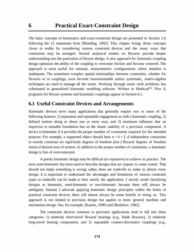
Two parallel blades, connected as shown in Figure 6-1, share a commontranslational degree of freedom. The rotational degrees of freedom of the individual bladesoccur about axes that are not in common, thus the combination of two blades constrainsthose degrees of freedom. Both blades redundantly constrain rotation about the translationalaxis. A displacement δz in the direction of freedom has an associated second-orderdisplacement δx given by Equation 6.1. This behavior is a general concern for all flexure
designs. All other constraint directions have nominally zero error, although geometrictolerances lead to very small errors that are first order with δz.
z
x
a
δ
δ
Figure 6-1 Two parallel blades allow one translational degree of freedom and constrain all others. Thisexample shows bolted construction but monolithic designs are also common.

Chapter 6 Practical Exact-Constraint Design
176
δ δx
a azz
xx
z
xx
a= − −
≅
=∫ ∫1 1
12
35
2
0
2
0
2dd
ddd
d (6.1)
Two cross blades, connected as shown in Figure 6-2, share one rotational degree offreedom. One blade constrains the degrees of freedom of the other that are not in common.Both blades redundantly constrain translation along the rotational axis. For a given rotationθ, each blade contributes a second-order radial displacement δr given by Equation 6.2. The
first term inside the braces is the chord across a deflected blade while the second term is thecomparable dimension produced by an ideal hinge. The net result is an extension rather thanforeshortening as in parallel blades. The total error is the vector sum from both blades.
δθ
θ θ θr a
a=
−
≅22 2 12
2
sin cos (6.2)
a
Figure 6-2 Two cross blades allow one rotational degree of freedom and constrain all others. Thisexample shows bolted construction but brazed connections are common in commercial products.
Blades arranged axially, as shown in Figure 6-3, share one rotational degree offreedom. Two blades in different planes are sufficient to constrain the remaining degrees offreedom, but a symmetrical design with four blades is more common. This arrangement hasnominally zero radial error motion in contrast to the cross-blade flexure. However,foreshortening of the blades in the axial direction presents an interesting compromise.Equation 6.3 shows the condition required to maintain equal foreshortening across thewidth of the blades. This condition is satisfied by joining the blades to parabolic-shapedflanges as Figure 6-3 (a) shows. Equation 6.4 shows the condition required to maintainequal bending stress across the width of the blades. The usual compromise solution is tojoin the blades to conical end caps as Figure 6-3 (b) shows. Making the blades relativelynarrow improves this compromise but reduces the stiffness and load capacity of the flexure.

6.1 Useful Constraint Devices and Arrangements
177
In addition, these equations suggest making the ratio a/r large, but they soon become invalidas the geometry diverges from normal beam theory. Finite element analysis is helpful incomputing the bending stresses, but a linear code will not represent foreshortening in theblades and the axial stress that may result.
δθ
a rr
aa r( ) ≅ ( ) → ∝
3
5
22 (6.3)
σθ
b rE t r
aa r( ) ≅ ( ) → ∝
32
2 (6.4)
a
r
(a)
a
r
(b)
Figure 6-3 Axial blades allow one rotational degree of freedom and constrain all others. The shape of theflanges is important to the behavior of the flexure. In (a), two paraboloids that share a common vertexsatisfy equal axial displacement across the blades. In (b), two cones that share a common vertex provide areasonable compromise between equal axial displacement and equal bending stress across the blades.
6.1.2 Basic Kinematic Couplings
A kinematic coupling provides rigid and repeatable connection between two objects throughusually six local contact areas. This is the case for the two traditional configurations shownin Figure 6-4: (a) the three-vee coupling and (b) the tetrahedron-vee-flat coupling (alsoknown as the Kelvin clamp). The weight of the object being supported or some otherconsistent nesting force holds the surfaces in contact. A spring or compliant actuator mayapply the nesting force, but ideally it should allow all surfaces to engage freely withminimum friction and wear. Otherwise, the coupling will not become centered as preciselyas it should or perhaps not at all. Friction between the contacting surfaces acting on thecompliance of the coupling is a main contributor to nonrepeatability as experimentallydetermined by [Slocum and Donmez, 1988].
The symmetry of three vees offers several advantages: better distribution of contactforces, better centering ability, thermal expansion about a central point and reducedmanufacturing costs due to identical features. Conversely, the tetrahedral socket offers a

Chapter 6 Practical Exact-Constraint Design
178
natural pivot point for angular adjustments. Many tip-tilt mirror mounts operate in thisfashion. The three-vee coupling is the natural choice for adjustments in six degrees offreedom or when there is no need for adjustment.
(a) (b)
Figure 6-4 In (a), the three-vee coupling has six constraints arranged in three pairs. In (b), the tetrahedron-vee-flat coupling has six constraints arranged in a 3-2-1 configuration. Often for manufacturing reasons, thetetrahedron is replaced with a conical socket, hence the more familiar name cone-vee-flat.
The local contact areas of the traditional kinematic couplings are quite small andrequire a Hertzian analysis to ensure a robust design for the chosen material pair (seeAppendix C, Contact Analysis). Greater durability is achieved by better curvature matchingbetween contacting surfaces. Rather than use a full sphere against a flat surface, a partialsphere of much larger radius may be used instead. The same applies to cylindrical surfacescontacting with crossed axes. Another approach is to use a full sphere against a concavespherical or cylindrical surface. Figure 6-5 compares these two approaches for a veeconstraint. Both constraints have the same relative (or effective) radius but the sphere in agothic arch has less capture range.
SR 1.225R .6capture capture
SR .5
Figure 6-5 A vee constraint showing two ways to increase the area of contact. Capture is the maximumdistance off center that the constraint will engage with tangency.

6.1 Useful Constraint Devices and Arrangements
179
Designs based on line contact rather than point contact offer a significant increase inload capability and stiffness. For example, line contact forms between a precisely made,heavily loaded sphere and conical socket. The kinematic equivalent to three vees is a set ofthree sphere-cone constraints with either the spheres or the cones supported on radial-motion flexures. The upper member in Figure 6-6 (a) has six rigid-body plus three flexuraldegrees of freedom that three cones exactly constrain. Alternatively in (b), the three-toothcoupling forms three theoretical lines of contact between cylindrical teeth on one memberand flat teeth on the other member. Each line constrains two degrees of freedom giving atotal of six constraints. Manufactured with three identical cuts directly into each member, theteeth must be straight along the lines of contact but other tolerances may be relatively loose.Both of these kinematic couplings are being used on the EUVL project to overcome thelimited hardness of super invar.
(a) (b)
Figure 6-6 In (a), flexure cuts in the upper member allow each sphere limited radial freedom to seat in theconical sockets of the lower member. In (b), the three-tooth coupling forms three theoretical line contactsbetween cylindrical teeth on one member and flat teeth on the other member.
6.1.3 Extensions of Basic Types
Arranging constraints is a design process that requires a basic understanding of kinematicsand the mechanics of constraint devices. The blade flexures and kinematic couplingspresented thus far are good examples from which to learn and start new designs. Thissection presents several interesting and useful extensions based on three vee constraints.The examples range from fairly direct implementation on a touch trigger probe to a lessobvious flexure stage with three degrees of freedom. In my experience, thinking of sixconstraints as three pairs has been a valuable and simplifying conceptual construct.
Chapter 6 Practical Exact-Constraint Design
180
6.1.3.1 Touch Trigger Probe
Touch trigger probes are commonly used on coordinate measuring machines to indicateprecisely where in the travel of the machine axes that contact is made with the workpiece. Itis sufficient if the probe signal occurs with a known position lag as this is easy to correct insoftware. A common design studied by [Estler, et al., 1996, 1997] employs a three-veekinematic coupling that acts as the electrical switch and the mechanical registration. Theproblem that Estler addresses through modeling and compensation is the variation inposition lag depending upon the direction of travel, the orientation of the surface and othereffects. A dominant error term, referred to as probe lobing, results from a three-foldvariation in the trigger force acting on the compliance of the probe shaft.
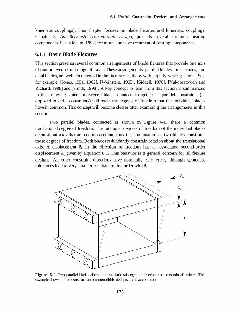
The heart of the problem is the orientation of the vee constraints. Figure 6-7 showsthe probe mechanism studied by Estler (a) and a new design (b) that solves probe lobing, atleast in theory. In (a), the probe side of the coupling is preloaded down by a compressionspring into three vee constraints represented by angled cylinders. The probe will not triggeruntil there is sufficient moment imparted to the coupling for any of the constraints tobecome unloaded, thus breaking electrical continuity. Although the preload is constant, thelever arm may vary up to a factor of two depending whether the coupling pivots about onevee or two. In (b), the new vee orientation requires a torsional preload to seat the coupling.In addition, the spring would be set to off-load the weight of the probe coupling. In thisconfiguration, any applied moment (orthogonal to the preload) equally unloads one side ofeach vee; there is no directional preference. The downside will be a greater influence offriction since any pin must now slide up or down a vee rather than simply lifting out.
Preload Force
(a)
Preload Torque
(b)
Figure 6-7 In (a), the moment required to unseat one vee while pivoting about the other two vees is afactor of two less than the moment required to unseat two vees while pivoting about the third vee. In (b), amoment applied about any axis in the plane of the vees produces equal reaction at all vees.

6.1 Useful Constraint Devices and Arrangements
181
6.1.3.2 The NIF Diagnostic Inserter
The NIF requires a number of diagnostic instruments near the center of the 10 m diametertarget chamber. Each instrument is transported approximately 6 m into the chamber by atelescoping diagnostic inserter. Since only the end position of travel requires submillimeterpositioning, a kinematic coupling is being considered to provide repeatable registration atthe end of a rather imprecise telescoping stage. However, the long, skinny geometry of theinserter presents an unfavorable aspect ratio for a traditional kinematic coupling. Theconfiguration shown in Figure 6-8 was proposed to work within the geometric constraintsyet provide acceptable moment stiffness and capacity. It was conceived by splitting the veesof a three-vee coupling and axially separating the odd-numbered constraints from the even-numbered constraints. The odd-numbered constraints act like a right-hand screw while theeven-numbered constraints act like a left-hand screw. An applied axial preload forcetranslates the cylinder until all constraints are engaged and an axial torque is establishedbetween the two sets of three constraints.
6
4
5
1
23
4
2
65
1
3
2
4
6
3
5
1Preload Force
Figure 6-8 The end view looks much like a three-vee coupling with constraint pairs 2-3, 4-5 and 6-1apparently forming three vees. The side view shows the significant separation between odd- and even-numbered constraints. As in Figure 6-7, the angled cylinders are constraints fixed to an unseen structure.

Chapter 6 Practical Exact-Constraint Design
182
6.1.3.3 The NIF optics assembly
The NIF requires many hundreds of kinematic couplings to support large, replaceableoptics assemblies. There are several types of kinematic couplings used throughout thesystem, but one in particular demonstrates a simple evolution from a basic three-veecoupling to a more novel configuration well suited for tall assemblies. Figure 6-9 shows theevolution in three simple steps. The horizontal configuration is convenient because gravityprovides the preload. Rotating the coupling to the vertical configuration has obviousconsequences, which motivates the next step to rotate the lower vees to carry the gravityload. It is important that the centroid of the supported object be offset from the lower vees ina direction that preloads the upper vee. The next step of spreading the upper vee has aparticular advantage for NIF optics assemblies. The widely spaced vee provides frictionalconstraint that stiffens the torsional vibration mode of the optics assembly. This exampleappears again in Section 6.3.3 and Chapter 7.
Spread the upper vee
Rotate the coupling
Rot
ate
the
low
er v
ees
Figure 6-9 The evolution from a horizontal three-vee coupling to the configuration used for many NIFoptics assemblies. The spheres in each configuration attach to the object being supported.

6.1 Useful Constraint Devices and Arrangements
183
6.1.3.4 EUVL Mirror Mount
Friction between the contacting surfaces of a kinematic coupling is a disadvantage when itcauses significant distortion in the precision component being supported. A commonapproach for mounting super-precision optics is an arrangement of three vee-flexures that[Vukobratovich and Richard, 1988] refer to as bipods. Figure 6-10 shows the bipod designused for EUVL mirror mounts. Each leg consists of four blades in series to provide oneconstraint and five degrees of freedom. One bipod provides the same constraint as a sphereand vee but without friction. Three bipods fully constrain the supported object with sixconstraints connected in parallel. Notice too that the top of the bipod has the features for athree-tooth coupling. There are mating features on the optic to provide the connect-disconnect function. The kinematic repeatability of the couplings ensure repeatable forcesimposed by the bipod flexures on the optic, leading to a repeatable distortion between opticmanufacturing and final use. This example appears again in Chapter 7 in greater detail.
Figure 6-10 A single bipod flexure constrains two degrees of freedom in the plane of the vee. Usually thecenter section connects to the precision component and the ends connect to the support. At times it may beadvantageous to reverse this role for better weight distribution provide by six supports.
6.1.3.5 X-Y-θθθθz Flexure Stage
A flexure stage that provides pure planar motion (X-Y-θz) satisfies a number of applications
found particularly in microelectronics and opto-mechanical systems. One approach to thisproblem is to serially connect single-axis flexure stages, for example, two sets of parallelblades and one set of cross blades. Besides being an awkward design, good stiffness ineach constraint direction is difficult to obtain. When possible, it is better to arrange

Chapter 6 Practical Exact-Constraint Design
184
constraints in parallel. An obvious example is a set of three single-constraint flexuresarranged physically parallel to each other. This arrangement is rigid and simple, but hassecond-order, out-of-plane error motion that can only be reduced with longer constraints. Abetter arrangement appears in Figure 6-11. It consists of three folded-hinge flexuresarranged as parallel constraints. This arrangement provides pure planar motion except forerrors arising from geometric tolerances.
Actuation Point(3) Places
Support (3) Places
y
x
z
Figure 6-11 Three folded hinge flexures constrain motion within a plane and provide convenient pointswith which to actuate the stage.
The folded hinge provides one constraint although it appears compliant in alldirections. Rather, the two blades have one degree of freedom in common so only five of thesix (2 x 3 DOF) are independent. One nice feature of the folded hinge is the convenientpoint to apply actuation, for example, with a micropositioner. This was the approach usedfor an EUVL X-Y stage that appears in Chapter 7. [Ryu, Gweon and Moon, 1997] designedan X-Y-θz wafer stage that uses piezoelectric actuators driving folded hinges.
6.2 Analytical Design of FlexuresMuch has been written about the analysis of flexures, so much so that the papers areseemingly saturated with the same information. There has been little new understandingpresented in resent years. The emphasis in this section is in providing new information andunderstanding. This is accomplished using both beam theory and finite element analysis. Afundamental contribution is a matrix-algebra technique for modeling flexure systems. Theequations for a blade flexure are contained in a compliance matrix and a stress matrix, bothof which consider column effects. This is a sophistication not found in the formulas ofSection 2.6. Computer software written for specific configurations such as the bipod flexurehas proved very valuable in the case studies for this thesis. A general-configuration programfor flexure systems, written in Mathcad Plus 6, appears in Section 6.3.

6.2 Analytical Design of Flexures
185
6.2.1 Comparison of Flexure Profiles
The blade flexures presented thus far have had constant thickness except perhaps near theends where small fillets are typical. Another common flexure profile is the circular hinge,which typically is manufactured by drilling two adjacent holes to form the flexure and thenby relieving other material as necessary to allow freedom of motion. The primary referencefor the circular hinge is [Paros and Weisbord, 1965]. More recently, the elliptical hinge wasstudied by [Xu and King, 1996] and [Smith et al., 1997]. When the thickness of the flexureis small compared to the circle or ellipse, both of these profiles are well approximated by aparabola. A parabolic profile leads to simpler equations and better understanding. Sincethese three profiles have effectively the same performance, the circular hinge is the obviouschoice for ease of manufacturing (whether by drilling holes or using circular interpolation).The interesting comparison is between the (circular, elliptical or parabolic) hinge flexure andthe blade flexure because each has particular advantages.
To remain the most general, the presentation uses the elliptical profile described bythe major and minor diameters a and b, respectively. For a circular profile, simply replaceboth a and b with the diameter d. Equation 6.5 gives the thickness profile for the ellipse andits approximate parabolic profile. Figure 6-12 compares these two profiles for an examplethat is near the limit for a good approximation. The approximation is better for a circularprofile and of course when the minimum thickness t0 is thinner. The straight lines in the
figure have to do with the comparison to the equivalent blade flexure discussed later.
t t bx
at
b x
ate p= + − −
≅ +
=0
2
0
2
1 12
22
(6.5)
5 4 3 2 1 0 1 2 3 4 50
1
2
3
t 0.0.5 t b
t e x
2
t p x
2
a b
2
a b
2
x
=a 10 =b 5 =t 0 1 =t b 1.262 =a b 7.49
Figure 6-12 The solid line indicates the profile for one side of an elliptical hinge flexure. The horizontalaxis is a plane of symmetry. The parabola (dash line) provides a good approximation in the thin region ofthe flexure that governs both the axial and moment compliance. The equivalent blade flexure is bounded bystraight lines indicated by ab and tb.
Equations 6.6 and 6.7 give simplified expressions for axial compliance and momentcompliance, respectively, for the parabolic profile. For this example, the axial compliance of

Chapter 6 Practical Exact-Constraint Design
186
the ellipse is underestimated by 3% and the moment compliance is overestimated by 5%compared to exact solutions using the elliptical profile. However, the use of beam theory inthe derivation is itself an approximation. These solutions are similar to those for the bladeflexure. If the blade were taken to be of length a and thickness t0, then the term in square
brackets would represent the factor by which the hinge flexure was different.
cE w
t xa
E w t
t
b
t
bx pa
a
= ≅ −
−
−∫1
22 21
2
2
0
0 0dπ
(6.6)
cE w
t xa
E w t
t
bpa
a
θ ν ν π= −( ) ≅ −( )
−
−∫1
121
12 316
22 3
2
22
03
0d (6.7)
It is instructive to consider the length and thickness of a blade that is equivalent tothe hinge flexure in terms of axial and bending compliance. The solution to two equationswith two unknowns appears in Equation 6.8, where the subscript b indicates the equivalentblade parameters. This explains the straight lines in the figure marked with either ab or tb.The line marked t0 indicates the part of the parabola that has the greatest slenderness ratio
for buckling. The usual definition for slenderness ratio is the length divided by theminimum radius of gyration. Here it is more convenient to use the length divided by thethickness. It is obvious from the figure that the equivalent blade being both longer andthinner is more likely to buckle under a compressive load. Equation 6.9 gives the conditionrequired for the hinge flexure to yield before buckling and the factor by which theequivalent blade flexure is more likely to buckle. For this example the factor is 1.88.
a
a
t
b
t
b
t
t
t
bb b≅ −
≅ −
163
22
2 163 2
20 03
0
0
ππ
ππ
(6.8)
SRa
t b
E SR
SR
t
bpy
b
p≅ < ≅ −
2 122
2
0
0πσ
π (6.9)
The hinge flexure clearly has the advantage over the blade flexure for bucklingresistance. The bending stress appears to be slightly higher for the thinner hinge flexure,since both equivalently require the same bending moment for a given rotation, but stressconcentrations in the fillets of the blades can be just as high. The main advantage for theblade flexure comes when there is need for rotational flexibility about the axis of the blade,so as to twist. Of course the hinge flexure is better if the application calls for resisting twist.This is also true if the flexure is to be used as a secondary constraint in shear.

6.2 Analytical Design of Flexures
187
6.2.2 A Study on Fillets for Blade Flexures
Beam theory works well for blade flexures except at each end where there is a transition tosome larger cross section. Monolithic blade flexures are usually manufactured with smallcorner radii know as fillets. Clamped blades, on the other hand, usually have very abrupttransitions that are difficult to model with any certainty. The edges of the clamping surfacesmay have partial radii to transition the clamping force, but it is assumed that microslip willrelieve the theoretically high stress concentration for axial and moment loads. Naturally thesubject of this study is the behavior of fillets as a function of radius size. This isaccomplished through a parameterized finite element model for one end of the blade.I In thestudy, the radius varies from one-half blade thickness to twice the blade thickness, and themodel is subject to either axial or moment loading. Curve fits to the finite-element resultsare useful to supplement the limitations of beam theory.
An assumption is made in beam theory that either the out-of-plane stress or the out-of-plane strain is zero. The same is true for 2D FEA. The two choices bracket the range of a3D model, plane stress for zero width and plane strain for infinite width. Both types werecompared to a 3D model of varying widths. Consistent with the general practice in flexuredesign, plane stress is most appropriate in the calculation of axial stiffness and stress due toaxial and moment loads. However, the results indicate that plane strain is more appropriatefor moment stiffness, contrary to general practice. The effect is rather small, only 5 to 10percent but in the nonconservative direction. Hence, the equations found in this thesis forbending of flexures have a factor (1 - ν2) to account for stiffening due to the Poissoneffect.II The same is true for the finite-element results that appear later in this section.
The shape of the transition region and the range of fillet radii are apparent in Figure6-13. In this case, an axial load is applied to the left end of the 20 x 20 block, and the rightend of the 2 x 10 blade is constrained. In Figure 6-14, opposite forces on the top andbottom of the block generate a moment load. Both figures show the deflected shape of themodel and contours of von Mises stress. Although difficult to see, the maximum stress foraxial loading occurs approximately at the quarter point of the fillet closest to the blade andoccurs very near the start of the fillet for moment loading. The node on the lower rightcorner of the block is the displacement location used for the compliance calculations. All theresults presented are normalized to the blade thickness t and calculations from beam theory.
I Pro/MECHANICA by Parametric Technology Corp. is the finite element software used in this study.II The bending stress across the thickness of the flexure changes from tension to compression over a veryshort distance. The blade would bow if not connected on each end to a stiff structure. The plane-strainassumption does not allow any bowing so the calculation underestimates the desired quantity, bendingcompliance. The blade has some opportunity to bulge in width when axially loaded. The plane-stressassumption freely allows bulging so the calculation underestimates the desired quantity, axial stiffness. Themaximum stress due to axial and moment loads occurs on the sides where the plane-stress assumption isvalid.

Chapter 6 Practical Exact-Constraint Design
188
Figure 6-13 The fillet radii shown here are one-half, one, three-halves and two times the blade thickness.The deflected shape and the contours of von Mises stress result from an axial load.
Figure 6-14 The fillet radii shown here are one-half, one, three-halves and two times the blade thickness.The deflected shape and the contours of von Mises stress result from a moment load.
The maximum stress from the 2D plane-stress model divided by the stresscalculated from beam theory is the stress concentration factor plotted in Figure 6-15 foraxial loading and Figure 6-16 for moment loading. In each graph, the solid line is a fittedcurve to discrete results from the finite element model. The equation at the top of each graphmay be used to calculate the stress concentration factor for any radius-to-thickness ratiobetween one-half and two. The knee in the curve appears to be at a ratio near one.

6.2 Analytical Design of Flexures
189
Axial Load
k = -0.1729(r/t)3 + 0.8539(r/t)2 - 1.4265(r/t) + 1.9613
1.00
1.05
1.10
1.15
1.20
1.25
1.30
1.35
1.40
1.45
0.50 0.75 1.00 1.25 1.50 1.75 2.00r / t
k =
st
ress
co
nce
ntr
atio
n
fact
or
Figure 6-15 The stress concentration factor for axial loading is closely approximated by a cubicpolynomial, where r/t is the ratio of fillet radius to blade thickness.
Moment Load
k = 0.1721(r/t)4 - 0.9288(r/t)3 + 1.8387(r/t)2 - 1.6593(r/t) + 1.669
1.00
1.02
1.04
1.06
1.08
1.10
1.12
1.14
1.16
1.18
1.20
0.50 0.75 1.00 1.25 1.50 1.75 2.00r / t
k =
st
ress
co
nce
ntr
atio
n
fact
or
Figure 6-16 The stress concentration factor for moment loading is closely approximated by a fourth-orderpolynomial, where r/t is the ratio of fillet radius to blade thickness.
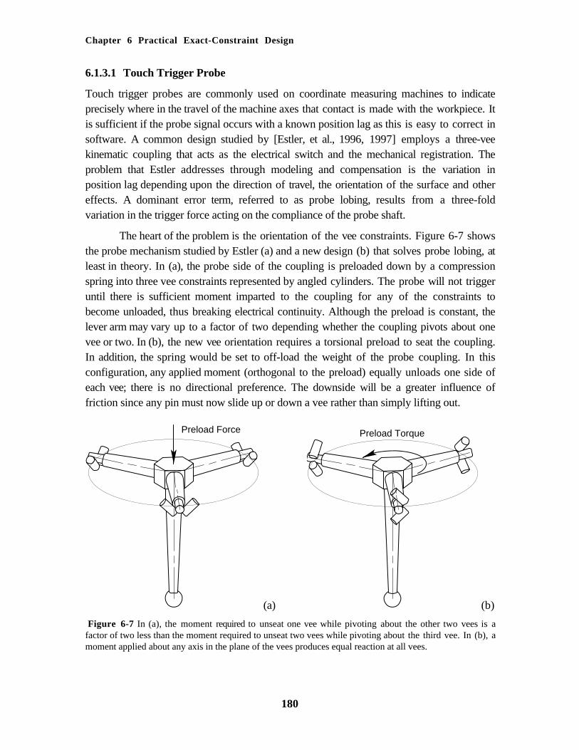
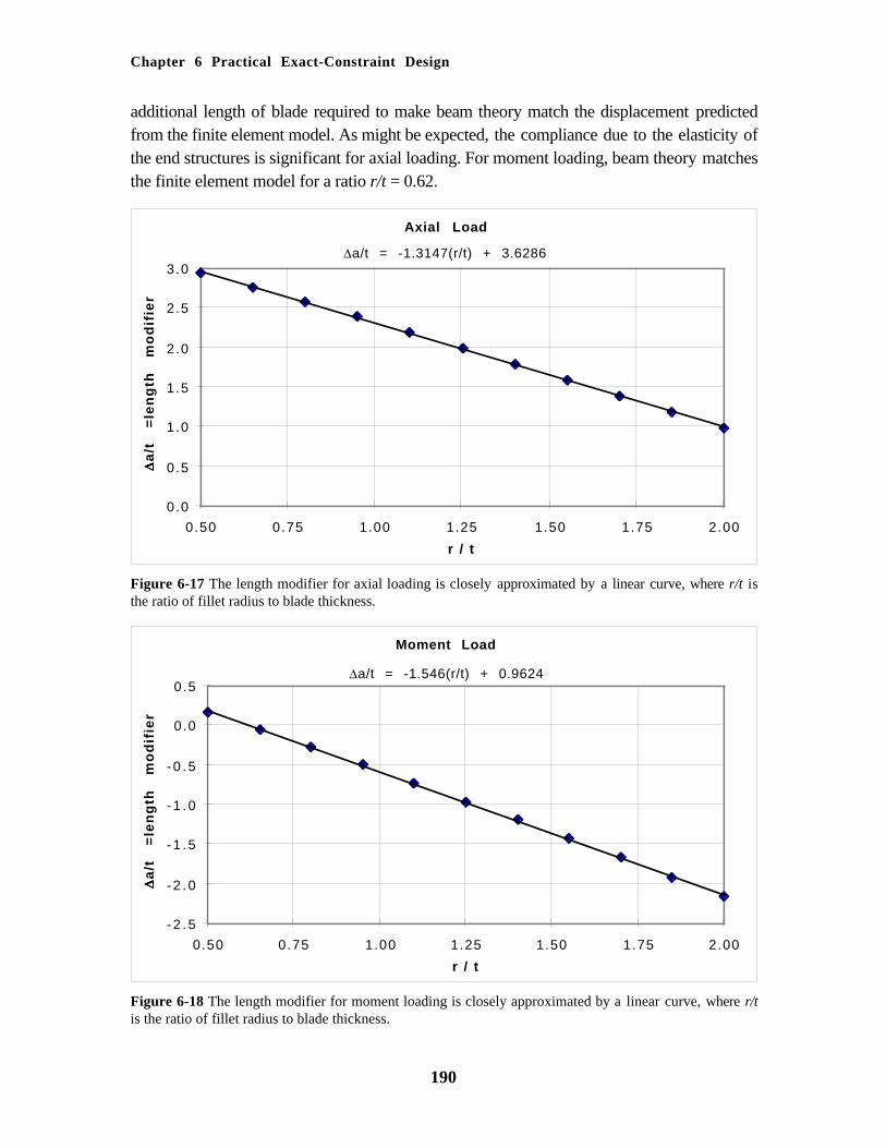
The size of the fillet radius also has an effect on the amount of deflection underload. A larger fillet shortens the effective length of the blade assuming that the endstructures remain separated by a constant distance a. This effect on blade length is apparentin Figure 6-17 for axial loading and Figure 6-18 for moment loading. The curves give the
Chapter 6 Practical Exact-Constraint Design
190
additional length of blade required to make beam theory match the displacement predictedfrom the finite element model. As might be expected, the compliance due to the elasticity ofthe end structures is significant for axial loading. For moment loading, beam theory matchesthe finite element model for a ratio r/t = 0.62.
Axial Load
∆a/t = -1.3147(r/t) + 3.6286
0.0
0.5
1.0
1.5
2.0
2.5
3.0
0.50 0.75 1.00 1.25 1.50 1.75 2.00
r / t
∆∆∆∆a
/t
=le
ng
th
mo
dif
ier
Figure 6-17 The length modifier for axial loading is closely approximated by a linear curve, where r/t isthe ratio of fillet radius to blade thickness.
Moment Load
∆a/t = -1.546(r/t) + 0.9624
-2 .5
-2 .0
-1 .5
-1 .0
-0 .5
0.0
0.5
0.50 0.75 1.00 1.25 1.50 1.75 2.00
r / t
∆∆∆∆a
/t
=le
ng
th
mo
dif
ier
Figure 6-18 The length modifier for moment loading is closely approximated by a linear curve, where r/tis the ratio of fillet radius to blade thickness.

6.2 Analytical Design of Flexures
191
6.2.3 The Compact Pivot Flexure
An axial arrangement of two blades in series is a useful single-constraint device thatprovides angular freedom about three axes. Since the two translational degrees of freedomare rather stiff for short blades, it is common to duplicate another set of two blades somedistance along the axial constraint direction. See, for example, the bipod flexure in Figure 6-16. The same cuts used to make the bipod flexure appear more clearly in Figure 6-19 (a).This basic design is being used on the NIF and EUVL projects. An advantage of this designbecomes apparent when compared to the more common design in (b), where the axialcompliance introduced at the junction between blades is significant. It clearly shows thecompromise between axial stiffness and how closely spaced the blades can be. The designshown in (a), with much deeper end sections, greatly relieves this compromise. Even so, itstarts to become an issue again when the blade is wider than four times its length. Thisthree-dimensional behavior is best studied with 3D finite element analysis. As before, finite-element results are displayed so as to extend the usefulness of simple theory.
(a) (b)
Figure 6-19 The design in (a) allows the minimum spacing of blades and maintains good axial stiffness.In addition, the gaps may be controlled to provide over-flexion protection. In order for the design in (b) tohave good axial stiffness, the junction between blades would have to be lengthened.
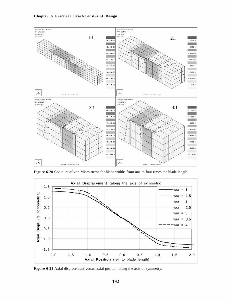
Since only axial displacement is of interest in this study, the use of symmetryboundary conditions at two midplanes simplifies the model to just one-quarter the physicalpivot flexure. This model, shown in Figure 6-20, also aids in viewing contours of von Misesstress through the blades. The variable parameter in this study is the blade width w, whichvaries from one to four times the length a. The blade length is ten times the thickness andthe fillet radius is one-half the blade thickness.
Although the blades become stiffer with increasing width, the aspect ratio of thejunction becomes less favorable and contributes a larger proportion to the total compliance.This is the reason in Figure 6-21 that the axial displacement when normalized to theoryincreases with blade width. This behavior is also apparent in von Mises stress as gradientsthat increase with blade width. Figure 6-22 shows how stress varies across the half-widthtaken through the center of the blade (length and thickness). Figure 6-23 shows how stressvaries along the axis of symmetry. Notice that these stresses are away from the stressconcentrations caused by fillets. A practical maximum for blade width is two times thelength partly because the torsional stiffness increases rapidly with the ratio w/a.
Chapter 6 Practical Exact-Constraint Design
192
Figure 6-20 Contours of von Mises stress for blade widths from one to four times the blade length.
Axial Displacement (along the axis of symmetry)
- 1 .5
-1 .0
-0 .5
0.0
0.5
1.0
1.5
-2 .0 -1 .5 -1 .0 -0 .5 0.0 0.5 1.0 1.5 2.0Axial Position (rel. to blade length)
Axi
al
Dis
pl.
(re
l. to
the
oret
ical
) w/a = 1
w/a = 1.5
w/a = 2
w/a = 2.5
w/a = 3
w/a = 3.5
w/a = 4
Figure 6-21 Axial displacement versus axial position along the axis of symmetry.
1:1 2:1
3:1 4:1

6.2 Analytical Design of Flexures
193
Von Mises Stress (across blade)
0.5
0.6
0.7
0.8
0.9
1.0
1.1
1.2
0.0 0.2 0.4 0.6 0.8 1.0Transverse Position (center to edge)
Vo
n
Mis
es
S
tre
ss
(r
el.
to
the
ore
tica
l)
w/a = 1
w/a = 1.5
w/a = 2
w/a = 2.5
w/a = 3
w/a = 3.5
w/a = 4
Figure 6-22 Von Mises stress versus position across the half width of the blade (taken at the mid length).
Von Mises Stress (along the axis of symmetry)
0.0
0.2
0.4
0.6
0.8
1.0
1.2
1.4
-2 .0 -1 .5 -1 .0 -0 .5 0.0 0.5 1.0 1.5 2.0
Axial Position (rel. to blade length)
Vo
n
Mis
es
S
tre
ss
(re
l. to
th
eo
retic
al)
w/a = 1
w/a = 1.5
w/a = 2
w/a = 2.5
w/a = 3
w/a = 3.5
w/a = 4
Figure 6-23 Von Mises stress versus position along the axis of symmetry.

Chapter 6 Practical Exact-Constraint Design
194
6.2.4 Helical Blades for a Ball-Screw Isolation Flexure
The rather specialized application of a ball-screw (or leadscrew) isolation flexure motivatedthe development of an analytical model for a mildly helical blade flexure. Isolation flexuresor bearing systems are commonly used on ultra-precision machines to couple only thedesirable degrees of freedom between a ball screw and the carriage it drives [Slocum, 1992].For different reasons, a recent paper demonstrated a clever way to improve the resolution ofa leadscrew by effectively placing a flexural leadscrew in series with the mechanicalleadscrew [Fukada, 1996], although no words to this effect are mentioned. While the screw-nut interface requires some level of torque before sliding takes place, the flexural leadscrewresponds to arbitrarily small torque to give arbitrarily small resolution. Both of thesevaluable functions, exact constraint and smaller resolution, can be achieved in one simpledevice using a set of helical blade flexures. This idea is being used on the NIF precisionlinear actuator (see Chapter 8.5).
Figure 6-24 The ball-screw flexure for the NIF precision actuator requires two rotational degrees offreedom, a primary constraint against translation along the screw, and secondary constraints for theremaining degrees of freedom. Note, some hidden lines were removed to better show the main features.
Figure 6-24 shows the basic flexure design used for the NIF actuator. It resemblesthe compact pivot flexure of the last section except that it is hollow to allow the ball screw topass through. In addition, the two hinge axes intersect to maximally condense the overalllength, but this is not required in general. On the NIF actuator, there is another pivot somedistance beyond the end of the screw so that the pivot pair provides free translation.Ordinarily the ball-screw flexure would have two pivots to provide free translation.Although it is not apparent from the figure, the blades are manufactured with a slight helixangle. Conceptually, if the blades were concentrated at the pitch diameter of the screw, thenthe proper helix angle would be perpendicular to the helix of the screw. Since the bladesmust lie outside the screw, then the actual helix angle must be somewhat smaller. This
6.2 Analytical Design of Flexures
195
condition does two things simultaneously: it aligns the blades to the reaction force; and italigns out-of-plane motion of the blades to an insensitive direction of the screw. Effectivelythis creates a flexural screw with the same lead as the mechanical screw. Either one or bothcan be active since they appear the same to the system.
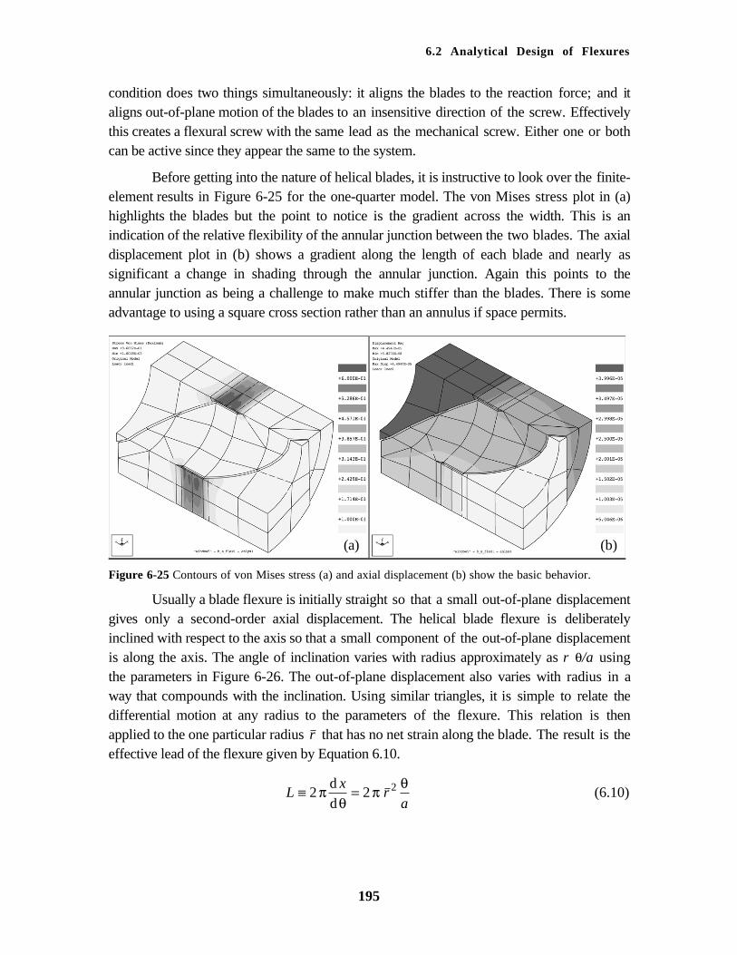
Before getting into the nature of helical blades, it is instructive to look over the finite-element results in Figure 6-25 for the one-quarter model. The von Mises stress plot in (a)highlights the blades but the point to notice is the gradient across the width. This is anindication of the relative flexibility of the annular junction between the two blades. The axialdisplacement plot in (b) shows a gradient along the length of each blade and nearly assignificant a change in shading through the annular junction. Again this points to theannular junction as being a challenge to make much stiffer than the blades. There is someadvantage to using a square cross section rather than an annulus if space permits.
Figure 6-25 Contours of von Mises stress (a) and axial displacement (b) show the basic behavior.
Usually a blade flexure is initially straight so that a small out-of-plane displacementgives only a second-order axial displacement. The helical blade flexure is deliberatelyinclined with respect to the axis so that a small component of the out-of-plane displacementis along the axis. The angle of inclination varies with radius approximately as r θ/a usingthe parameters in Figure 6-26. The out-of-plane displacement also varies with radius in away that compounds with the inclination. Using similar triangles, it is simple to relate thedifferential motion at any radius to the parameters of the flexure. This relation is thenapplied to the one particular radius r that has no net strain along the blade. The result is theeffective lead of the flexure given by Equation 6.10.
Lx
ra
≡ =2 2 2πθ
π θdd
(6.10)
(a) (b)

Chapter 6 Practical Exact-Constraint Design
196
θ
r ww2
1
a
Figure 6-26 The effective lead of a helical blade flexure is governed by the parameters a, w1, w2, and θ.
To go further requires an assumption that the ends are constrained to remainparallel. Again using similar triangles, it is simple to determine the axial strain at any radius.Since the flexure is in equilibrium, the axial strain integrated over the cross section must bezero as indicated in Equation 6.11. Upon solving, Equation 6.12 gives the radius for zerostrain, which then may be substituted back into Equation 6.10.
0
1
2
1
2
1
22 2
2 2 2 22 2= =
−( )+ ( )
≅
+ ( )−( )∫ ∫ ∫∂ε
∂θ
θ
θθ
θr
r
r
r
r
r
rr r
a rr
a rr r rd d d (6.11)
r r r r r w w w w212
1 2 22
12
1 2 221
316
≅ + +( ) = + +( ) (6.12)
The axial strain that results from the helical shape also acts to stiffen the flexure intorsion beyond that for a flat blade. The approach used in Equation 6.13 to compute thiseffect is essentially a strain energy method (Castigliano’s first theorem). The additionaltorsional stiffness due solely to the helix correctly goes to zero as the lead of the screw goesto zero.
k E t a r E t aa r
r r r
E t w w
a
w w w w
w w w w
r
L
helix
r
r
r
r
θ∂ε∂θ
θθ
π
=
≅
+ ( )
−( )
≅−( ) + +
+ +
∫ ∫2 2
124 7 45 5 5
2
2
2 2
22 2 2
2 13
12
1 2 22
12
1 2 22
1
2
1
2
d d
++
−L
r2
2
π
(6.13)

6.2 Analytical Design of Flexures
197
6.2.5 A General Approach for Analyzing Flexure Systems
The most general approach for analyzing a flexure system is finite element analysis.Arbitrarily large, complex systems to very simple systems are readily modeled withcommercial FEA software. For example, blade flexures typically modeled with shellelements are connected as necessary to other shell and/or solid elements to represent thewhole system. It is hard to imagine a more flexible way to accurately analyze deflectionsand stresses in some spatially complex arrangement of flexures. Yet in several respects theapproach presented here is more flexible than FEA especially early in the design cycle. Themodel is completely parametric and represents only the elements of interest, usually theflexures. It reports the stiffness and compliance matrices for the constrained system, and itincludes column effects that a linear FEA code cannot. The main drawback is that the usermust understand the basics of matrix algebra and transformation matrices, which istransparent to the user of an FEA code.
The basic assumption is that the flexure system can be modeled as parallel andseries combinations of springs and that an equivalent spring for the system representsuseful information, for example, the stiffness matrix. If desired, that information can bepropagated back to individual springs, for example, to obtain local forces and moments. Thekey formalism in this approach is the six-dimensional vector used to succinctly representthree linear degrees of freedom and three angular degrees of freedom. We will deal strictlywith force-moment vectors and differential displacement-rotation vectors. These vectors arerelated through the stiffness matrix or the compliance matrix of the spring. The concept of athree-dimensional stiffness matrix as expressed in Equation 6.14 may be more familiar. Thesix-dimensional stiffness matrix is assembled as blocks of three-dimensional matrices asEquation 6.15 shows. At times it may be easier to start by building the compliance matrix asin Equation 6.16. Converting from one to the other requires inverting the whole matrixrather than inverting separate blocks.
f Kf/=
=
⋅
= ⋅f
f
f
k k k
k k k
k k k
x
y
z
xx xy xz
xy yy yz
xz yz zz
x
y
z
d
d
d
d
δδδ
δ δ (6.14)
f
m
K K
K KK Kf/ f/
m/ m/m/ f/
=
⋅
=δ θ
δ θδ θ
δθ
d
dT (6.15)
d
dTδ
θδ δ
θ θθ δ
=
⋅
=C C
C C
f
mC C/f /m
/f /m/f /m (6.16)
Once the stiffness matrix or the compliance matrix is formed in one coordinatesystem (CS), it is a simple matter using the [6 x 6] transformation matrix to reflect it to anyanother (CS). Once expressed in the same CS, stiffness matrices are added to represent

Chapter 6 Practical Exact-Constraint Design
198
parallel combinations, and compliance matrices are added to represent series combinations.This process is expressed in Equations 6.17 and 6.18 (also A.35 and A.36). Mixedcombinations of parallel and series springs require like groups to be combined first theninverted as necessary to complete the combination. See Appendix A for a completediscussion of transformation matrices and parallel and series combinations.
K T K T0 0 0= ⋅ ⋅∑ / /T
i i ii
(6.17)
C T C T0 0 01= ⋅ ⋅− −∑ /
T/i i i
i
(6.18)
The remainder of this section focuses on the details that make this approach trulyuseful. The first task is to derive the compliance matrix for the blade flexure. The solutiondepends on the CS so naturally we will choose the simplest one. Similarly, the stress matrixis derived so that maximum stresses in the blade are easy to calculate. Finally the details ofconstructing parallel-series spring models are presented.
6.2.5.1 The Compliance Matrix for a Blade Flexure
a
w
t
y'
y
z'
z
x'
x
Figure 6-27 Imagining the CS’s as rigid links to the ends of the blade, the application of forces andmoments at these CS’s results in respective displacements and rotations with no coupling between axes.
The flexion of a blade may be represented as movement between two CS’s that attach toopposite ends of the blade. It would be more common to place a CS at each end but it ismore convenient to place them initially coincident with the principal axes of the blade. Thena blade undergoing flexion appears as slightly displaced CS’s in Figure 6-27. In similarfashion, the forces and moments may be represented about these CS’s rather than at theends where they are physically applied. This choice of CS’s diagonalizes the compliance

6.2 Analytical Design of Flexures
199
matrix. Four of the six diagonal elements appear already in Chapter 2.6 as stiffnesses butwithout derivation or explanation. Here we go through each element with due care and addmore generality with column effects and side-by-side blades. As in Figure 6-26, w2 is theoutside dimension of blades and w1 is the inside dimension. In addition, it is necessary to
represent the width of the individual blades or of a single blade as w.
We begin with the in-plane constraint directions. Axial compliance is the firstdiagonal element in the compliance matrix (6.19) and is so familiar that it needs noexplanation. It is linear in all the key parameters and therefore is convenient for normalizingthe other compliances. The second diagonal element (6.20) corresponds to a y-directionforce, which produces combined bending and shear in the blade. It comes from the familiarfixed-guided beam equation and has an added term for the shear deformation. The sectionproperties have been simplified for the side-by-side blade geometry. The last constraintdirection is also the last element in the compliance matrix (6.21). Here the blade is in purebending due to a moment about the z axis.
C1 12 1
, = =−( )c
a
E t w wx (6.19)
C2 2
2
12
1 2 22 2 4 1, .= =
+ ++ +( )
c ca
w w w wy x ν (6.20)
C6 612
1 2 22
12, = =
+ +c
c
w w w wz
xθ (6.21)
The remaining diagonal elements are out-of-plane directions usually considered asdegrees of freedom. The elements corresponding to z and θy directions are similar to y andθz directions from before and differ mainly in a factor t 2 in the denominator rather than w2.
However, there are two subtle distinctions. As noted earlier in Section 6.2.2, the equationsfor bending compliance should include a factor (1 - ν2) to account for the Poisson effect.The other factor is the effect of an axial force, either compressive or tensile. The solutionsfor fixed-guided and cantilever boundary conditions are available from numerous sources,for example, [Vukobratovich and Richard, 1988], [Young, 1989] and [Smith, 1998].Unfortunately the equations are not particularly convenient or intuitive, involvingtrigonometric functions for compression and hyperbolic functions for tension. Uponsubstituting power series approximations, the two types of functions become the same whenexpressed with a positive or negative axial force. The number of terms required in the powerseries depends upon how closely the flexure operates to the critical buckling load. We willkeep enough terms to have good accuracy through one-half the critical load.
The third diagonal element for the z-direction force (6.22) follows from the seriesapproximation of the axially loaded, fixed-guided beam. The effect of the axial force iscontained within the square brackets. As expected, the compliance decreases for a positive
Chapter 6 Practical Exact-Constraint Design
200
tensile force and increases for a negative compressive force. The approximation differs fromthe exact solution by only 6.6% at one-half the critical load. Usually we would not venturethis close to buckling unless the intent is a zero-stiffness condition. Then it is necessary touse the exact solution from the references.
C3 32
22 3
2
2
1 165
1735
62315
2 4 1
12
, .= ≅ −( )
− + −
+ +( )
≡ =
c ca
t
f c a
t
z x
x xcr
ν γ γ γ ν
γ γ π(6.22)
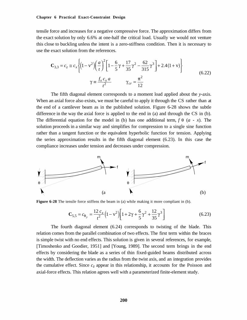
The fifth diagonal element corresponds to a moment load applied about the y-axis.When an axial force also exists, we must be careful to apply it through the CS rather than atthe end of a cantilever beam as in the published solution. Figure 6-28 shows the subtledifference in the way the axial force is applied to the end in (a) and through the CS in (b).The differential equation for the model in (b) has one additional term, f θ (a - x). Thesolution proceeds in a similar way and simplifies for compression to a single sine functionrather than a tangent function or the equivalent hyperbolic function for tension. Applyingthe series approximation results in the fifth diagonal element (6.23). In this case thecompliance increases under tension and decreases under compression.
ff
mm
θθ
Figure 6-28 The tensile force stiffens the beam in (a) while making it more compliant in (b).
C5 5 22 2 312
1 1 265
1235, = = −( ) + + +
cc
ty
xθ ν γ γ γ (6.23)
The fourth diagonal element (6.24) corresponds to twisting of the blade. Thisrelation comes from the parallel combination of two effects. The first term within the bracesis simple twist with no end effects. This solution is given in several references, for example,[Timoshenko and Goodier, 1951] and [Young, 1989]. The second term brings in the endeffects by considering the blade as a series of thin fixed-guided beams distributed acrossthe width. The deflection varies as the radius from the twist axis, and an integration providesthe cumulative effect. Since cz appear in this relationship, it accounts for the Poisson and
axial-force effects. This relation agrees well with a parameterized finite-element study.
(b)(a

6.2 Analytical Design of Flexures
201
C4 4
212
1 2 22 1
121
2 14 2 52, .= =
+( )+
+ + +
−
ct
w
t
c
w w w w
cxx z
θ ν(6.24)
6.2.5.2 The Stress Matrix for a Blade Flexure
The distribution of stress through a blade varies greatly depending on the direction of theapplied force or moment. For purposes of sizing the blade, however, it is sufficient toconsider only the maximum absolute value of stress resulting from applied forces andmoments. This information may be represented in a diagonal matrix similar to thecompliance matrix. The judicious choice of the CS causes symmetric distributions of stressdue to individual components of the force-moment vector. Each distribution will have themaximum absolute value of stress always extending to the eight corners of the blade. Thereis one worse-case corner where all the stresses are in general alignment (perfectly aligned ifnot for shear stresses). Then a somewhat conservative estimate of the combined maximumabsolute principle stress is the simple sum of the individual maximum’s as calculated fromthe stress matrix multiplied by the applied force-moment vector.
In keeping with the order presented for the compliance matrix, the three terms thatcorrespond to constraint directions are considered first for the stress matrix. The firstdiagonal element for axial loading (6.25) is simply the inverse of the cross sectional area. Itis convenient to use for scaling the other terms. For the second diagonal element (6.26), they-direction force produces combined bending and shear in the blade. A somewhatconservative approach treats the maximum absolute value of principle stress as if alignedwith the x-axis. This simplifies the final step of combining all the stress components butyields a slightly higher combined stress than a more rigorous analysis. The last constraintdirection and also the last element in the stress matrix (6.27) is much simpler because theblade is in pure bending from a z moment.
S1 12 1
1, = =
−( )st w wx (6.25)
S2 22
12
1 2 22
2
12
1 2 22
23
2
3
21, = =
+ +( ) ++ +( )
+
s sa w
w w w w
a w
w w w wy x (6.26)
S6 62
12
1 2 22
6, = =
+ +s s
w
w w w wz xθ (6.27)
The stresses due to the remaining three elements usually result due to requiredmotions of the flexure but they will be written for applied loads. The third diagonal element(6.28) corresponds to a z-direction force. Although the blade experiences combinedbending and shear loading, the shear stress is usually not significant given normal blade

Chapter 6 Practical Exact-Constraint Design
202
proportions. It is excluded in preference of keeping a simple expression for the columneffect from an axial force. As expected the bending stress increases with a negativecompressive force and decreases with a positive tensile force. The fifth diagonal elementcorresponds to a y-moment (6.29) and exhibits slightly more complicated behavior. Theaxial force causes the bending moment to be nonsymmetric along the length of the blade.I
The bending moment is maximum at the fixed end for tension and minimum forcompression. The use of the singularity function in the equation turns off the effect of acompressive force when γ is negative, leaving just the applied moment as the maximum.
S3 32 33
165
5135, = = − + −
s sa
tz x γ γ γ (6.28)
S5 51 2 36
1 6 6125, = = + + +
s sty xθ γ γ γ (6.29)
As described in the previous section, there are two effects to consider when a bladetwists on axis. The first is simple twist with no end effects. The shear stress produced ismaximum far away from the corners and therefore may be safely ignored. The other effectis bending of the blade as a fixed-guided beam with the maximum stress occuring at thecorners. The fourth diagonal element (6.30) represents this effect by using sz as thereference rather than sx. As a result it also represents column effects.
S4 42
12
1 2 22
6, = =
+ +s s
w
w w w wx zθ (6.30)
The stress matrix multiplied by the force-moment vector gives a vector of stresscomponents that may be positive or negative depending on the loading. It is useful to look ateach component to understand which loads are most significant. The worse-case stress isconservatively estimated by summing the absolute values of the stress components.
6.2.5.3 Parallel-Series Spring Models
The use of parallel and series combinations of springs is fairly common in engineeringanalysis. Working in 6-D is certainly less common but the basic concept of parallel-seriescombinations is no different. Most of the gritty details are in the matrix algebra carried outby the computer. The most challenging aspect usually is in setting up the transformationmatrices. Perhaps the best way to understand the modeling aspect is to work through anexample step by step. The X-Y-θz flexure stage, shown in Figure 6-11 on page 184, is a
good example to represent several levels of parallel and series combinations of springs.
I The asymmetry of the bending moment is a consequence of the way the blade is loaded along the x axis ofone CS. A symmetric bending moment would result if the axial force bisected the x axes of both CS’s.This symmetric case is more appropriate for the cross blade flexure but not for more general arrangements.

6.2 Analytical Design of Flexures
203
Figure 6-29 shows the spring model of the same flexure stage with three actuators. Thesteps required to set up and analyze the model are enumerated below.
z
x
y
9
8
7
65
4
1
2 3
Figure 6-29 The X-Y-θz flexure stage appearing in Figure 6-11 is modeled with nine springs in parallel
and series combinations as shown.
a) Identify the main member (the thing being moved or supported) and attach the basecoordinate system CS0 at a convenient location. It is simple to reflect the results to a
different CS if desired.
b) Identify all the separate paths from the main member to ground. There are six in theexample, three flexure supports and three actuators.
c) Identify and number each spring in each path. There are nine in the example, six bladesand three actuators.
d) Assign a unique CS to each spring. Number these CS1 to CSn. Then create [6 x 6]
transformation matrices to represent the spatial relationships between the local CS’s andthe base CS0.
e) Create as many compliance matrices as required to represent all the springs with respectto their own local CS’s. There are only two for the example, one matrix for six identicalblades and one matrix for three identical actuators.
f) Reflect the compliance matrix for each spring to the base CS0 using the transformationmatrices, thus creating n unique compliance matrices. Number these C1 to Cn.
g) Identify the springs that form either series or parallel combinations. When reflected tothe same CS, series springs experience the same load while parallel springs experiencethe same deflection. The example has three sets of parallel springs, 2-3, 5-6 and 8-9.

Chapter 6 Practical Exact-Constraint Design
204
h) Add the stiffness matrices of springs in parallel and add the compliance matrices ofsprings in series. Indicate these new equivalent springs by the spring numbers theyrepresent. The equivalent springs for the example are K2-3, K5-6, and K8-9.
i) Repeat steps 7 and 8 using the equivalent springs in place of the ones they represent.Stop when there is only one equivalent spring remaining. The example requires a totalof three combination steps before reaching the equivalent spring for the system. Thesecond step is a series combination resulting in C1-2-3, C4-5-6, and C7-8-9. The last step isa parallel combination resulting in K0, the equivalent spring for the system.
There are a number of uses for the system stiffness and compliance matrices.Presumably there is some requirement that drives the design to have a certain level ofstiffness in the constraint directions and certain freedoms in other directions. Specific loadcases may be applied to ascertain deflections or certain motions may be specified todetermine resulting reaction forces. The sizes and locations of blades are easily modified toevaluate design changes. Details about individual blades such as stresses or reaction forcesrequire the applied load or specified motion to be propagated back through the combinationprocess, being careful to apply loads to springs in series or motions to springs in parallel. Aclearly labeled sketch of the model for each step in the combination process will help avoidconfusion and mistakes.
The fine details of these analysis steps appear in the flexure system analysisprogram in Section 6.3. The program documents the example of the X-Y-θz flexure stage
discussed here. In particular it shows how to set up the [6 x 6] transformation matrices andreflect compliance matrices to the base CS0. It also shows how easily a fairly complex
system of blades is modeled with parallel and series combinations of springs.
A slightly more advanced topic is the modeling of column effects in a system offlexures. It was not an important effect in the X-Y-θz flexure stage so it was not introduced
then. The compliance matrix and the stress matrix for individual blades account for localcolumn effects, but it is necessary to include the system effects at the system level.Fortunately this is straightforward to do with additional springs that represent the columnbehavior. This behavior may occur when a series combination carries a significant axialforce, for example, when two blades lie in the same plane so as to act like one much longerblade. The effect of the axial force is modeled with a new spring placed in parallel with theseries combination. The stiffness of the new spring depends only on the axial force and thedistance between the two CS’s of the series combination, as in Equation 6.31. It may bepositive or negative for a tensile or compressive force, respectively. When reflecting thisstiffness to the base CS0, the transformation matrix should be the same as the most mobile
blade in the series combination. Then it may be combined as any of the other springs.
K3 3, = f
Lx (6.31)

205
6.3 Friction-Based Design of Kinematic CouplingsI
Friction affects several aspects important to the design of kinematic couplings, butparticularly the ability to reach the centered position is fundamental. It becomes centeredwhen all constraints are fully engaged even though a small uncertainty may exist about theideal center where potential energy is minimum. For many applications, centering ability is agood indicator for optimizing the coupling design. Typically, the coupling design processhas been largely heuristic based on a few guidelines [Slocum, 1992]. Symmetric forms ofthe basic kinematic couplings are simple enough to develop closed-form equations forcentering ability. More general configurations lacking obvious symmetries are difficult tomodel in this way. A unique kinematic coupling for large, interchangeable optics assembliesin the NIF motivated the development of computer software to optimize centering ability.The program, written in Mathcad Plus 6, appears in Section 6.3.
6.3.1 Friction Effects in Kinematic Couplings
Friction affects at least four important characteristics of a kinematic coupling as indicated byorder-of-magnitude estimates that all include the coefficient of friction µ. These estimatesare listed in Equations 6.32 through 6.35 and are described below.
Repeatabilityf
k R
P
E≈
µ 2
3
1 3 2 3
(6.32)
Kinematic support f ft n≤ µ (6.33)
Stiffness k kf
fkt n
t
nn= −
−−
≈2 22
1 0 831 3
νν µ
. (6.34)
Centering abilityf
fc
n≈ −0 5 1 3. . µ (6.35)
Tangential friction forces at the contacting surfaces may vary in direction andmagnitude depending how the coupling comes into engagement. This affects therepeatability of the coupling and the kinematic support of the precision component. Theestimate for repeatability is the unreleased frictional force multiplied by the coupling’scompliance. The estimate is derived as if the coupling’s compliance in all directions is equalto a single Hertzian contact carrying a load P and having a relative radius R and elasticmodulus E. The frictional force acts to hold the coupling off center in proportion to thecompliance. This estimate will underestimate the repeatability if the structure of the couplingis relatively compliant compared to the contacting surfaces.
I This material was previously published in condensed form [Hale, 1998].

Chapter 6 Practical Exact-Constraint Design
206
Kinematic support is important for stability of shape of the precision componentbeing supported by the coupling. The estimate for kinematic support simply gives a boundon the magnitude of friction force acting at any contact surface. A sensitivity analysis of theprecision component will determine a tolerable level of friction that the coupling can have.This may drive the design to include flexure elements and/or procedures to release storedenergy. If repeatable engagement is not so important, then constraints using rolling-elementbearings offer very low friction. For example, a pair of cam followers that contact withcrossed axes is equivalent to a sphere on a flat but with twenty or more times less friction.
In some cases frictional overconstraint is valuable for increasing the overall systemstiffness. Provided the tangential force is well below what would initiate sliding, thetangential stiffness of a Hertzian contact is comparable to the normal stiffness [Johnson,1985]. This motivated the widely spaced vee used to stiffen the first torsional mode of NIFoptics assemblies (see Figure 6-9).
Centering ability can be expressed as the ratio of centering force to nesting force.The estimate provided is typical for a symmetric three-vee coupling. A larger ratio means thecoupling is better at centering in the presence of friction. It is also convenient to expresscentering ability as the coefficient of friction where this ratio goes to zero. For the estimate,the limiting coefficient of friction is 0.5/1.3 = 0.38. The coupling will center if the realcoefficient of friction is less than the limiting value.
6.3.2 Centering Ability of the Basic Kinematic Couplings
We begin by studying the centering ability of the basic kinematic couplings because theirgeometry is relatively simple and familiar. When brought together initially off center, theconstraints engage sequentially as the coupling seeks a path to center.I This path becomesbetter defined as more constraints engage. For example, five constraints allow the couplingto slide along one well-defined path. Four constraints allow motion over a two-dimensionalsurface of paths and so forth. Although there are infinitely many paths to center, only thelimiting case is of practical interest for determining centering ability. Further, it is reasonableto expect the limiting case to be one of six possible paths that have five constraintsengaged.II This point will be demonstrated using examples and simple logic.
The simplest example is the symmetric three-vee coupling. Figure 6-30 shows twoways that the coupling may slide to center depending on its initial misalignment. In (a), twovee constraints are fully engaged and the third is off center giving a total of five constraints.The two vees define an instantaneous center of rotation. The off-center vee transforms itsshare (one-third) of the nesting force into a centering moment about the instant center.
I It is a rare possibility that initial contact can occur at two places simultaneously.II The exception to this statement is the ball-cone constraint since the cone provides only one constraintuntil the ball is fully seated. A tetrahedral socket remedies this situation.

6.3 Friction-Based Design of Kinematic Couplings
207
Equation 6.36 describes the centering force at the center of the coupling due to this moment,where α is the angle to each surface from the plane of the vees. This path is the limiting casealong with five other symmetrically identical paths.I In (b), two off-center vees transformtheir share (two-thirds) of the nesting force into a centering force given by Equation 6.37.This causes the coupling to translate along the fully engaged vee. With only fourconstraints, the coupling is also free to roll but there is no moment in this direction. Givenfreedom like this, the coupling will move in the general direction of the centering force untilthe next constraint engages and forces it along a more resistive path to center.
f
fc
n= −
+( ) −sin coscos sin cos
α µ αα µ α
µα2
33
(6.36)
f
fc
n= + −
+ +( ) −3 4 3 4
3 4 3 3 3
2
2
sin tan
cos tan tan cosα α µ
α α µ α
µα
(6.37)
(a) (b)
Figure 6-30 In (a), the three-vee coupling slides on five constraints producing rotation about an instantcenter. In (b), the coupling slides on four constraints in the general direction of the centering force.
The three-tooth coupling behaves similarly to the three-vee coupling, but thecentering force with five constraints engaged is very difficult to model in closed form. Table6-1 shows the limiting coefficient of friction for both three-vee and three-tooth couplings ascalculated by the kinematic coupling analysis program. There is negligible differencebetween the two types over the range 45˚ to 55˚. The three-vee coupling has slightly bettercentering ability at the nearly optimal angle of 60˚. With only four constraints engaged, thecentering force causes simple translation of the three-tooth coupling, which leads to areasonable closed-form solution given by Equation 6.38. Graphs of Equations 6.36, 6.37and 6.38 versus the coefficient of friction µ appear in Figure 6-32 (a). The point to notice isthat the centering force decreases when the fifth constraint engages.
I The coupling may rotate clockwise or counterclockwise about any of three instant centers.

Chapter 6 Practical Exact-Constraint Design
208
Angle of Inclination α 45˚ 50˚ 55˚ 60˚ 65˚
Three-Vee Coupling 0.317 0.338 0.354 0.364 0.365
Three-Tooth Coupling 0.319 0.339 0.351 0.352 0.339
Table 6-1 The limiting coefficient of friction versus angle for three-vee and three-tooth couplings.
f
fc
n= + −
+ +( )sin tan
cos tan tan
α α µ
α α µ α
4 4
2 4
2
2(6.38)
An aspect hidden by the symmetry in the previous examples is the possibility that apath with five constraints engaged may have greater centering force than a different pathwith only four constraints. However as the coupling continues toward center, the centeringforce cannot increase as the fifth constraint engages. The tetrahedron-vee-flat couplingexhibits behavior of the type shown in Figure 6-32 (b). Usually the centering ability will belimited by the path shown in Figure 6-31 (a). The centering force for this path is given inEquation 6.39, where α is the vee angle and β is the tetrahedron angle. The opposite-direction path has one less constraint and greater centering force as described by Equation6.40. This solution is also representative of the cone-vee-flat coupling. However in Figure6-31 (b), a different path with five constraints has typically greater centering force asdescribed by Equation 6.41. The main point is that all six paths having five constraintsengaged must be considered to determine centering ability.
(a) (b)
Figure 6-31 The tetrahedron-vee-flat coupling has six unique paths having five constraints engaged. Thepath in (a) usually limits the centering ability of the coupling. The path in (b) could limit the centeringability if the vee angle is too shallow.
f
fc
n=
+ −
+ +( ) − −sin tan
cos tan tan cos
β β µ
β β µ β
µα
µ4 4
6 4 3 3
2
2(6.39)
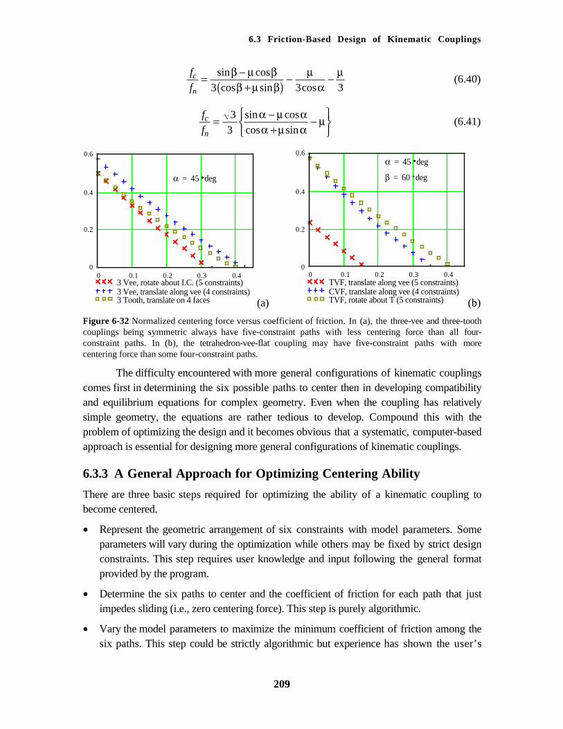
6.3 Friction-Based Design of Kinematic Couplings
209
f
fc
n= −
+( ) − −sin coscos sin cos
β µ ββ µ β
µα
µ3 3 3
(6.40)
f
fc
n= −
+−
33
sin coscos sin
α µ αα µ α
µ (6.41)
0 0.1 0.2 0.3 0.40
0.2
0.4
0.6
3 Vee, rotate about I.C. (5 constraints)3 Vee, translate along vee (4 constraints)3 Tooth, translate on 4 faces
=α 45 deg
(a)
0 0.1 0.2 0.3 0.40
0.2
0.4
0.6
TVF, translate along vee (5 constraints)CVF, translate along vee (4 constraints)TVF, rotate about T (5 constraints)
=α 45 deg
=β 60 deg
(b)
Figure 6-32 Normalized centering force versus coefficient of friction. In (a), the three-vee and three-toothcouplings being symmetric always have five-constraint paths with less centering force than all four-constraint paths. In (b), the tetrahedron-vee-flat coupling may have five-constraint paths with morecentering force than some four-constraint paths.
The difficulty encountered with more general configurations of kinematic couplingscomes first in determining the six possible paths to center then in developing compatibilityand equilibrium equations for complex geometry. Even when the coupling has relativelysimple geometry, the equations are rather tedious to develop. Compound this with theproblem of optimizing the design and it becomes obvious that a systematic, computer-basedapproach is essential for designing more general configurations of kinematic couplings.
6.3.3 A General Approach for Optimizing Centering Ability
There are three basic steps required for optimizing the ability of a kinematic coupling tobecome centered.
• Represent the geometric arrangement of six constraints with model parameters. Someparameters will vary during the optimization while others may be fixed by strict designconstraints. This step requires user knowledge and input following the general formatprovided by the program.
• Determine the six paths to center and the coefficient of friction for each path that justimpedes sliding (i.e., zero centering force). This step is purely algorithmic.
• Vary the model parameters to maximize the minimum coefficient of friction among thesix paths. This step could be strictly algorithmic but experience has shown the user’s

Chapter 6 Practical Exact-Constraint Design
210
intelligence to be very valuable. Keeping the user in the loop builds intuition andunderstanding of the tradeoffs involved.
These three steps are explained through the example that motivated this work, the NIFoptics assembly.
Orthographic and isometric views of one NIF optics assembly, discussed previouslyin Section 6.1.3.3 and again in Chapter 7, appear in Figure 6-33. The six constraints thatkinematically support the optics assembly are represented in the figure by reaction forcevectors numbered 1 to 6. In the model, each constraint is represented by a simple springstiffness defined along the z-axis of a local x-y-z coordinate system (CS). The use of six-dimensional vectors and [6 x 6] transformation matrices completely automates thedevelopment of compatibility and equilibrium equations, but the local CS’s can bechallenging to set up even for experienced users. See Appendix A for a complete discussionof transformation matrices.
In the program, two equations completely define the local CS’s for any arrangementof six constraints. Equation 6.42 defines the overall transformation matrix as a series ofsimple transformations: x-y-z translation, z rotation, y rotation and x rotation. The user mustdecide the proper number and order of simple transformations for the application, butusually there will be six parameters, p1 through p6. These parameters come from the column
of Equation 6.43 that corresponds to the particular constraint under consideration. In theexample, the CS definition for constraint 1 is: rotate θ2 about global x, rotate -θ1 about
global y, and translate in global x-y-z (-0.385, -0.315, -0.8). An equivalent definition is:translate in local (initially global) x-y-z (-0.385, -0.315, -0.8), rotate -θ1 about local y, androtate θ2 about local x. During the optimization, constraints 1 and 3 symmetrically changeorientation according to θ1 and θ2. Similarly, constraints 2 and 4 change according to θ1 andθ3, and constraints 5 and 6 change according to θ4. The user determines the number of
variable parameters used in the optimization. In addition, the user must supply the nestingforce vector and a vector of spring stiffnesses, one for each constraint.
T p ...T xyz ,,p1 p2 p3 R z p6 R y p5 R x p4 (6.42)
P θ
0.385
0.315
0.8
θ2
θ1
0
0.385
0.315
0.8
θ3
θ1
0
0.385
0.315
0.8
θ2
θ1
0
0.385
0.315
0.8
θ3
θ1
0
0.397
0.241
0.85
.90 deg
0
θ4
0.397
0.241
1.31
.90 deg
0
θ4 (6.43)

6.3 Friction-Based Design of Kinematic Couplings
211
W
1, 343
Y
X
XY
Z
W
6
5
21
W
Y
Z Z
X
6
5
2, 4
1
5
6 4
2
3
5
6
21 3
4
Figure 6-33 Orthographic and isometric views of one NIF optics assembly. The arrows numbered 1-6represent the six constraints that support the assembly. The arrows are proportional to the reaction forces.
The second step uses the constraint arrangement, the nesting force vector andconstraint stiffnesses to determine the six paths to center and the coefficient of friction foreach path that yields zero centering force. If the constraint arrangement is truly kinematic,then the parallel combination of six constraint stiffnesses will form a [6 x 6] stiffness matrixfor the coupling that is full rank. Equation 6.17 (also A.35) on page 198 expresses the

Chapter 6 Practical Exact-Constraint Design
212
process of reflecting the stiffness matrix from a local CSi to a global CS0 then summing allthe reflected stiffness matrices. Since there is only one nonzero term in Ki, the matrixequation reduces to an outer product of the third column of T0/i times the simple stiffness.
The technique used to find the vector direction for sliding is rather elegant. Adegenerate stiffness matrix is computed for only five constraints engaged. This matrix hasfive nonzero eigenvalues (if the coupling is truly kinematic). The eigenvector correspondingto the zero eigenvalue gives the direction in the global CS that the coupling will slide for thatparticular set of five constraints. This procedure is executed six times, once for eachconstraint not engaged.
The procedure used to determine the coefficient of friction for zero centering forceis coded in just three expressions but becomes rather complicated to explain. It should helpto review the comments and equations in the program. Starting with one sliding vector in theglobal CS, the same transformation matrices are used to create six local sliding vectors, onefor each constraint. Then a six-dimensional, force-moment vector is calculated for eachconstraint using the Coulomb law of friction and a unit normal force. Transforming back tothe global CS, the vectors are assembled into a matrix that when multiplied by a vector ofnormal forces (i.e., the contact force for each constraint) gives the resultant force-momentvector for the coupling. The inverse of this matrix is useful because it takes the appliedforce-moment vector (i.e., the nesting force) and gives back the contact forces for a givencoefficient of friction. Finally, the row of this matrix equation corresponding to theconstraint not engaged is solved for the coefficient of friction that makes its normal forcezero. This gives the coefficient of friction that just impedes sliding. This procedure isexecuted six times, once for each constraint not engaged. The minimum of six results is thelimiting coefficient of friction for the particular constraint arrangement.
The last step is to adjust the constraint arrangement in a manner that maximizes thelimiting coefficient of friction. The user presumably has set up the program to include somenumber of variable parameters given by the vector θ. The optimization approach is agraphical technique that provides the user with sufficient visual feedback to find theoptimum within a few iterations. The user must enter three vectors: the nominal vector θ andthe range for the graph, θmin and θmax. For each parameter, the program generates one
curve over its range while holding all other parameters at their nominal values. All curvesappear in one graph versus a normalized range of model parameters. The user adjusts thenominal values attempting to maximize the limiting coefficient of friction.
Figure 6-34 shows two graphs for the NIF optics assembly with slightly differentnominal parameters. The horizontal dashed line indicates the limiting coefficient of frictionfor the nominal parameter set. The optimal parameter set is apparent in (a) because a changeto any one parameter reduces the limiting coefficient of friction. It is useful to observe thesuboptimal parameter set in (b). By adjusting the nominal values towards the peaks in thecurves, the user soon converges to the optimal parameter set.

6.3 Friction-Based Design of Kinematic Couplings
213
0 0.2 0.4 0.6 0.8 10.25
0.3
0.35
0.4
min µ θ
< >µ r1
< >µ r2
< >µ r3
< >µ r4
=T
θ 40 25 45 60 deg
(a) 0 0.2 0.4 0.6 0.8 10.25
0.3
0.35
0.4
min µ θ
=T
θ 45 35 45 60 deg
(b)
Figure 6-34 Limiting coefficient of friction versus a normalized range of model parameters. Each curvecorresponds to one individually varying parameter with the others held constant at nominal values. Thehorizontal dashed line indicates the nominal parameter set. The graph in (a) shows the optimal configurationwhile (b) is suboptimal. In this example, the markers occur in 5˚ increments of the angle parameters.
6.4 Mathcad Documents for Generalized Kinematic Modeling
The Mathcad computing environment is ideal for engineering analysis where it is importantfor the user to understand the mechanics of the program. All the code is in plain sight and infamiliar mathematical format. It is easy to add text and drawings to better explain how to usethe program, usually referred to as a document.
6.4.1 Flexure System Analysis ProgramThis program helps the user develop a parameterized model of a flexure system so that sizesand locations of blades may be chosen to achieve key performance requirements. Eachblade in the system is represented by the compliance matrix of a spring in a local coordinatesystem (CS). All blades are then reflected to a common CS to allow simple addition ofcompliance matrices for springs in series or of stiffness matrices for springs in parallel. Theend result is the equivalent compliance matrix for the system and its reciprocal, the stiffnessmatrix. Applied loads or specified motions may then be applied to these matrices todetermine the resulting behavior. Loads may be propagated back to local blades todetermine the maximum stresses.
This program uses six dimensional vectors and [6 x 6] matrices to deal simultaneously withboth linear and angular measures. The first three components correspond to linear measuressuch as force and displacement, and the last three correspond to angular measures such asmoment and rotation. The same arrangement applies to the rows and columns of thematrices used for coordinate transformation, stiffness and compliance. In addition, thepositions and orientations for an arbitrary number n of flexure blades are convenientlystored in an [m x n] matrix. Each column describes a sequence of moves (typically m = 6)required to go from the global X-Y-Z CS to a local x-y-z CS as shown in the figure. Thismatrix may also contain parameters that the user may vary to optimize the configuration.

Chapter 6 Practical Exact-Constraint Design
214
Forces and displacements for the flexure system are represented in the global CS whileforces and displacements at a particular flexure are represented in its local x-y-z CS.
The transformations between the X-Y-Z CS and x-y-z CS's are done as a sequence ofmoves. The number and order may vary to suit the application, but they must be the samefor each flexure since they are stored in a matrix. The basic moves are: translation in x-y-z,rotation about x, rotation about y and rotation about z. The sequence may be interpreted asmoves relative to the base CS or in the opposite order as moves relative to the local CS. Tworules express these interpretations for a sequence of transformation matrices: 1) postmultiply to transform in the local CS and 2) pre multiply to transform in the base CS. Atypical sequence relative to the base CS is: rotate about the X axis, rotate about the Y axis,rotate about the Z axis, and translate (X, Y, Z). The equivalent sequence relative to the localCS is: translate (x, y, z) (initially coincident with the base CS), rotate about the z axis, rotateabout the y axis, and rotate about the x axis. The transformation matrix for this sequence isTXYZ RZ RY RX.
Enter each blade parameter in a row vector with as many columns as unique blades.
E 200000 Elastic modulus
ν 0.3 Poisson ratio
a 20
w 40
t 0.5
k act 0
r
x
w
t
z
a
y
XY
Z
Define below the transformation matrix T(p) for the particular sequence of moves to be used. For each local x-y-z CS, enter values of moves that define it in the corresponding column of the position matrix P below. Include any parameters in the position matrix as desired to aid in changing the configuration.
T p ...R z p6 T xyz ,,p1 p2 p3 R z p5 R x p4 b 100
P
0
b
0.90 deg
0.240 deg
.0.5 a
ba
2
0.90 deg.90 deg.240 deg
0
b
0
0
0.240 deg
0
b
0.90 deg
0
0
.0.5 a
ba
2
0.90 deg.90 deg
0
0
b
0
0
0
0
0
b
0.90 deg
0.120 deg
.0.5 a
ba
2
0.90 deg.90 deg.120 deg
0
b
0
0
0.120 deg

6.4 Mathcad Documents for Generalized Kinematic Modeling
215
Expressed in the base CS, the rotation matrix transforms either a force-moment vector or a differential displacement-rotation vector in the new CS to the base CS. Being orthonormal, the transposed rotation matrix gives the inverse transformation. The translation matrix is not orthonormal and transforms only a force-moment vector in the new CS to the base CS. The transposed translation matrix transforms only a differential displacement-rotation vector in the base CS to the new CS. The same applies to a general [6 x 6] transformation matrix.
R x x
1
0
0
0
0
0
0
cos x
sin x
0
0
0
0
sin x
cos x
0
0
0
0
0
0
1
0
0
0
0
0
0
cos x
sin x
0
0
0
0
sin x
cos x
[6 x 6] rotation matrix for rotation about the x-axis.
R y y
cos y
0
sin y
0
0
0
0
1
0
0
0
0
sin y
0
cos y
0
0
0
0
0
0
cos y
0
sin y
0
0
0
0
1
0
0
0
0
sin y
0
cos y
[6 x 6] rotation matrix for rotation about the y-axis.
R z z
cos z
sin z
0
0
0
0
sin z
cos z
0
0
0
0
0
0
1
0
0
0
0
0
0
cos z
sin z
0
0
0
0
sin z
cos z
0
0
0
0
0
0
1
[6 x 6] rotation matrix for rotation about the z-axis.
T xyz ,,x y z
1
0
0
0
z
y
0
1
0
z
0
x
0
0
1
y
x
0
0
0
0
1
0
0
0
0
0
0
1
0
0
0
0
0
0
1
[6 x 6] translation matrix for translation in x, y and z.
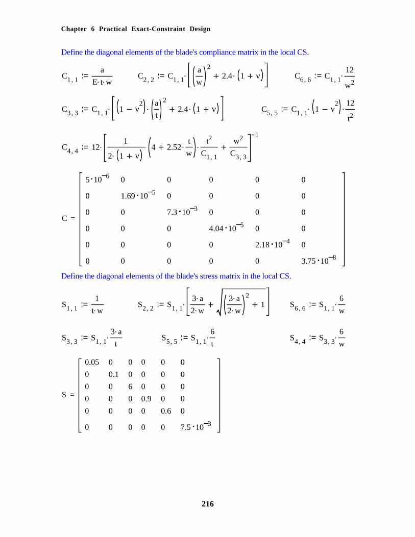
Chapter 6 Practical Exact-Constraint Design
216
Define the diagonal elements of the blade's compliance matrix in the local CS.
C ,1 1
a..E t w
C ,2 2.C ,1 1
a
w
2.2.4 1 ν C ,6 6
.C ,1 1
12
w2
C ,3 3.C ,1 1
.1 ν2 a
t
2.2.4 1 ν C ,5 5
..C ,1 1 1 ν2 12
t2
C ,4 4.12 ..1
.2 1 ν4 .2.52
t
w
t2
C ,1 1
w2
C ,3 3
1
=C
5 10 6
0
0
0
0
0
0
1.69 10 5
0
0
0
0
0
0
7.3 10 3
0
0
0
0
0
0
4.04 10 5
0
0
0
0
0
0
2.18 10 4
0
0
0
0
0
0
3.75 10 8
Define the diagonal elements of the blade's stress matrix in the local CS.
S ,1 1
1.t w
S ,2 2.S ,1 1
.3 a.2 w
.3 a.2 w
2
1 S ,6 6.S ,1 1
6
w
S ,3 3.S ,1 1
.3 a
tS ,5 5
.S ,1 1
6
tS ,4 4
.S ,3 3
6
w
=S
0.05
0
0
0
0
0
0
0.1
0
0
0
0
0
0
6
0
0
0
0
0
0
0.9
0
0
0
0
0
0
0.6
0
0
0
0
0
0
7.5 10 3

6.4 Mathcad Documents for Generalized Kinematic Modeling
217
Reflect the compliance and stiffness matrices from the local CS j to the base CS.
K b j ..T < >P j C 1T
T < >P j C b j K b j 1
K a j ..< >
T < >P j 1k act
T< >T < >P j 1
C a j K a j 1
Combine parallel and series combinations.
K 2_3 K b 2 K a 3 C 2_3 K 2_31
K 5_6 K b 5 K a 6 C 5_6 K 5_61
K 8_9 K b 8 K a 9 C 8_9 K 8_91
C 1_2_3 C b 1 C 2_3 K 1_2_3 C 1_2_31
C 4_5_6 C b 4 C 5_6 K 4_5_6 C 4_5_61
C 7_8_9 C b 7 C 8_9 K 7_8_9 C 7_8_91
K 0 K 1_2_3 K 4_5_6 K 7_8_9 C 0 K 01
=C 0
3.89 10 3
0
0
0
0
0
1.78 10 15
3.89 10 3
0
0
0
0
0
0
1.37 10 5
0
0
0
0
0
0
2.72 10 9
0
0
0
0
0
0
2.72 10 9
0
0
0
0
0
0
3.73 10 7
=K 0
256.94
5.48 10 11
0
1.53 10 9
1.25 10 9
3.48 10 9
1.18 10 10
256.94
0
1.25 10 9
1.53 10 9
3.56 10 8
0
0
7.28 104
7.72 10 7
6.01 10 6
3.06 10 9
1.53 10 9
1.25 10 9
7.73 10 7
3.68 108
3 10 4
0
1.25 10 9
1.53 10 9
6.01 10 6
3 10 4
3.68 108
0
4.66 10 9
3.86 10 8
3.06 10 9
0
0
2.68 106
Chapter 6 Practical Exact-Constraint Design
218
6.4.2 Kinematic Coupling Analysis ProgramThis program helps the user develop a parameterized model of a kinematic coupling so thatits ability to reach a seated position may be optimized. The coupling reaches a seatedposition when all six constraint surfaces are contacting. It approaches the seated positionfrom one of several directions determined by the surfaces already in contact. The limitingcase will always occur with five surfaces in contact, and there are only six such directions.The program determines the six directions then solves for the corresponding coefficients offriction that just impede sliding. The smallest coefficient of friction among the six is thelimiting coefficient of friction. The program varies parameters between limits set by the userand plots the limiting coefficient of friction. This visual feedback helps the user find theglobal optimum for this highly coupled, nonlinear problem. In addition, the programcalculates the following items for the optimized coupling assuming zero friction: stiffnessand compliance matrices, coupling displacement, and contact forces. Due to lengthycalculations, it is advisable to set automatic calculation off.
This program uses six dimensional vectors and [6 x 6] matrices to deal simultaneously withboth linear and angular measures. The first three components correspond to linear measuressuch as force and displacement, and the last three correspond to angular measures such asmoment and rotation. The same arrangement applies to the rows and columns of thematrices used for coordinate transformation, stiffness and compliance. In addition, thepositions and orientations for six constraint surfaces are conveniently stored in a matrixwith six columns. Each column describes a sequence of moves required to go from theglobal X-Y-Z CS (coordinate system) to a local x-y-z CS as shown in the figure. Thismatrix also contains the parameters that the program varies in the optimization process.Forces and displacements for the kinematic coupling are represented in the global CS whileforces and displacements at a particular constraint are represented in its local x-y-z CS. Thez direction represents the outward facing normal of the fixed surface so that a negativedisplacement is movement of the coupling into contact.
The transformations between the X-Y-Z CS and x-y-z CS's are done as a sequence ofmoves. The number and order may vary to suit the application, but they must be the samefor each constraint since they are stored in a matrix. The basic moves are: translation in x-y-z, rotation about x, rotation about y and rotation about z. The sequence may be interpreted asmoves relative to the base CS or in the opposite order as moves relative to the local CS. Tworules express these interpretations for a sequence of transformation matrices: 1) postmultiply to transform in the local CS and 2) pre multiply to transform in the base CS. Atypical sequence relative to the base CS is: rotate about the X axis, rotate about the Y axis,rotate about the Z axis, and translate (X, Y, Z). The equivalent sequence relative to the localCS is: translate (x, y, z) (initially coincident with the base CS), rotate about the z axis, rotateabout the y axis, and rotate about the x axis. The transformation matrix for this sequence isTXYZ RZ RY RX.
Define below the transformation matrix T(p) for the particular sequence of moves to beused. For each local x-y-z CS, enter values of moves that define it in the correspondingcolumn of the position matrix P(θ) below. Include components of the parameter vector θ inthe position matrix to allow optimization of the coupling.

6.4 Mathcad Documents for Generalized Kinematic Modeling
219
T p ...T xyz ,,p1 p2 p3 R z p6 R y p5 R x p4
P θ
0.385
0.315
0.8
θ2
θ1
0
0.385
0.315
0.8
θ3
θ1
0
0.385
0.315
0.8
θ2
θ1
0
0.385
0.315
0.8
θ3
θ1
0
0.397
0.241
0.85
.90 deg
0
θ4
0.397
0.241
1.31
.90 deg
0
θ4
Enter a vector k of contact stiffnesses and a vector f of forces and moments applied to the coupling at the origin of X-Y-Z. Note, a transformation matrix may be used to apply the force elsewhere.
k
1
1
1
1
1
1
f
0
0
450
0
0
0
z
yx
XY
Z
Expressed in the base CS, the rotation matrix transforms either a force-moment vector or a differential displacement-rotation vector in the new CS to the base CS. Being orthonormal, the transposed rotation matrix gives the inverse transformation. The translation matrix is not orthonormal and transforms only a force-moment vector in the new CS to the base CS. The transposed translation matrix transforms only a differential displacement-rotation vector in the base CS to the new CS. The same applies to a general [6 x 6] transformation matrix.
R x x
1
0
0
0
0
0
0
cos x
sin x
0
0
0
0
sin x
cos x
0
0
0
0
0
0
1
0
0
0
0
0
0
cos x
sin x
0
0
0
0
sin x
cos x
[6 x 6] rotation matrix for rotation about the x-axis.
R y y
cos y
0
sin y
0
0
0
0
1
0
0
0
0
sin y
0
cos y
0
0
0
0
0
0
cos y
0
sin y
0
0
0
0
1
0
0
0
0
sin y
0
cos y
[6 x 6] rotation matrix for rotation about the y-axis.

Chapter 6 Practical Exact-Constraint Design
220
R z z
cos z
sin z
0
0
0
0
sin z
cos z
0
0
0
0
0
0
1
0
0
0
0
0
0
cos z
sin z
0
0
0
0
sin z
cos z
0
0
0
0
0
0
1
[6 x 6] rotation matrix for rotation about the z-axis.
T xyz ,,x y z
1
0
0
0
z
y
0
1
0
z
0
x
0
0
1
y
x
0
0
0
0
1
0
0
0
0
0
0
1
0
0
0
0
0
0
1
[6 x 6] translation matrix for translation in x, y and z.
A coupling with only five surfaces in contact is free to slide in one direction. In this direction, the stiffness matrix is singular, assuming zero friction. The eigenvector of the stiffness matrix corresponding to the zero eigenvalue provides the direction of sliding, although it may have the wrong sign. The stiffness matrix K for the coupling is a summation of contact stiffnesses transformed to the global CS. The definition of K below excludes the jth contact surface from the sum. Use j = 0 to calculate K with all surfaces in contact. The matrix ∆ contains the six sliding directions in its columns, all relative to the global CS.
K ,P j
= 1
6
i
...< >
T < >P i 3ki i j
T< >T < >P i 3
∆ P for
< >∆
ieigenvec ,K ,P i 0
∈i ..1 6
∆
The coefficient of friction that just impedes sliding causes the coupling to be in static equilibrium. Obviously the non contacting surface has zero normal force. Therefore, static equilibrium equations can be solved to determine the coefficient of friction that makes the normal force zero at the surface intended to be noncontacting. This first requires a relationship for the friction force. Given a sliding direction δ and a coefficient of friction µ, the vector φ is a normalized force-moment vector that includes tangential friction. Both δ and φ are defined in the local x-y-z CS. Transformed to the global CS , φ's for all six contact surfaces are assembled in matrix A. Matrix A multiplied by a six-component vector of surface normal forces equals the resultant force-moment vector for the coupling.
φ ,δ µ
T.µ δ
1
Tδ
1δ
2δ
3
.µ δ2
Tδ
1δ
2δ
3
1 0 0 0

6.4 Mathcad Documents for Generalized Kinematic Modeling
221
A ,,P δ µ for
< >A i .T < >P i φ ,.T
T < >P i δ µ
∈i ..1 6
A
Since matrix A is invertible, the surface normal forces are linearly solved from the applied force-moment vector f. The only one of interest is the surface intended to be non contacting, which is zero at equilibrium. The root of this nonlinear equation provides the coefficient of friction that just impedes sliding. The coefficients of friction for all six sliding directions are assembled in vector µ.
µ 0 Starting value for the solver.
µ ,P ∆ for
µi
root ,lsolve ,A ,,P< >
∆i
µ fi
µ
∈i ..1 6
µhe program plots curves of the limiting coefficient of friction over ranges of parameters that vary
ndividually. Each curve is a function of one parameter while the others are held at nominal values. The ser will adjust the nominal set towards the optimal set. Enter minimum and maximum values for the arameter ranges to plot. Enter the nominal parameter set. Enter the number of points to plot over the ange (typically n r := 5). Enter the number of parameters (typically n p := rows(θ) but may be fewer). tart the calculation (command =) if in manual mode.
θ min.
35
15
30
45
deg θ max.
55
35
50
65
deg θ .
40
25
45
60
deg =θ θ min
θ max θ min
0.25
0.5
0.75
0.75
n r 5 i ..1 n r P θ P θα
i
i 1
n r 1n p 4 j ..1 n p =rank K ,P θ 0 6
θ r ,i j θ r θ
θ rj
.1 αi
θ minj
.αi
θ maxj
θ r
µ θ µ ,P θ ∆ P θ
=µ θ
0.391
0.445
0.53
0.441
0.378
0.387µ r
,i jmin µ ,P θ r ,i j ∆ P θ r ,i j
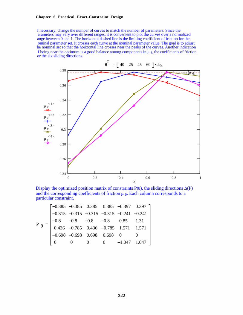
Chapter 6 Practical Exact-Constraint Design
222
f necessary, change the number of curves to match the number of parameters. Since the arameters may vary over different ranges, it is convenient to plot the curves over a normalized ange between 0 and 1. The horizontal dashed line is the limiting coefficient of friction for the ominal parameter set. It crosses each curve at the nominal parameter value. The goal is to adjust he nominal set so that the horizontal line crosses near the peaks of the curves. Another indication f being near the optimum is a good balance among components in µ θ, the coefficients of friction or the six sliding directions.
0 0.2 0.4 0.6 0.8 10.24
0.26
0.28
0.3
0.32
0.34
0.36
0.38min µ θ
< >µ r
1
< >µ r2
< >µ r3
< >µ r
4
α
=T
θ 40 25 45 60 deg
Display the optimized position matrix of constraints P(θ), the sliding directions ∆(P) and the corresponding coefficients of friction µ θ. Each column corresponds to a particular constraint.
=P θ
0.385
0.315
0.8
0.436
0.698
0
0.385
0.315
0.8
0.785
0.698
0
0.385
0.315
0.8
0.436
0.698
0
0.385
0.315
0.8
0.785
0.698
0
0.397
0.241
0.85
1.571
0
1.047
0.397
0.241
1.31
1.571
0
1.047

6.4 Mathcad Documents for Generalized Kinematic Modeling
223
=∆ P θ
0.322
0.121
0.325
0.229
0.318
0.789
7.232 10 3
0.2
0.276
0.193
0.02
0.92
0.341
0.222
0.361
0.097
0.295
0.779
0.034
0.203
0.275
0.189
1.307 10 3
0.92
0.392
0.525
0.207
0.656
0.311
0
0.378
0.531
0.209
0.664
0.3
0
=T
µ θ 0.391 0.445 0.53 0.441 0.378 0.387
Display a vector of surface normal forces, the couplings displacement, and the stiffness and compliance matrices.
f norm lsolve ,A ,,P θ 0 0 f K θ K ,P θ 0 C θ K θ1
=Tf norm 180.844 169.289 203.765 168.51 83.822 68.812 =.C θ f
1.809
57.505
317.867
94.622
17.728
23.375
=K θ
2.592
0
0
0.199
0.245
0.42
0
1.857
0.179
0.489
0.199
0
0
0.179
1.551
0.345
0
0
0.199
0.489
0.345
1.542
0.43
2.349 10 3
0.245
0.199
0
0.43
3.559
0.487
0.42
0
0
2.349 10 3
0.487
0.346
=C θ
0.544
0.01
4.02 10 3
0.023
0.155
0.878
0.01
0.625
0.128
0.249
0.084
0.132
4.02 10 3
0.128
0.706
0.21
0.039
0.052
0.023
0.249
0.21
0.815
0.133
0.165
0.155
0.084
0.039
0.133
0.419
0.778
0.878
0.132
0.052
0.165
0.778
5.048

224