6 P. M. Evans 1 2 3 7 Barsoum 10 11 SO40 7HU, UK. 12 13 ...10.1038/s41598-017... · 7 Barsoum 4, J....

Supplementary Information 1

for 2

‘Thresholds of biodiversity and ecosystem function in a forest ecosystem undergoing 3

dieback’ 4

5

P. M. Evans1, A. C. Newton1, E. Cantarello1, P. Martin1, N. Sanderson2, D. L. Jones3, N. 6

Barsoum4, J. E. Cottrell4, S. W. A'Hara4, L. Fuller5 7

1Centre for Conservation Ecology and Environmental Sciences, Faculty of Science and 8

Technology, Bournemouth University, Poole, BH12 5BB, UK. 9

2Botanical Survey and Assessment, 3 Green Close, Woodlands, Southampton, Hampshire, 10

SO40 7HU, UK. 11

3School of Environment, Natural Resources and Geography, Bangor University, Gwynedd, 12

LL57 2UW, UK. 13

4Forest Research, Alice Holt Lodge, Farnham, Surrey, GU10 4LH, UK. 14

5Biological and Environmental Sciences, University of Stirling, Stirling, FK9 4LA, UK. 15

Tel +44 (0) 1202 961831 16

[email protected] 17

18

19

Inventory of Supplementary Information: 20

Table S1: Basal area statistics. 21

Fig. S1: Graph of stand basal area over the dieback gradient. 22

Fig. S2: Non-threshold relationships between stage of dieback and ecosystem processes. 23

Supplementary Methods, SM1: Additional methods for experimental design and most data 24

collection. 25

Supplementary Methods, SM2: Methods for collecting and analysing ground-dwelling 26

arthropods data. 27

Table S2: Summary of variables measured and units used. 28

Table S3: Generalised linear mixed models used for the study and their results. 29

Table S4: Updated version of Table S3 with only linear and quadratic term of BA included as 30

fixed effects. 31

Table S5: Statistics of the soil properties. 32

Supplementary Methods, SM3: Graphs to support the space-for-time assumption. 33

34

35

Fig. S1: The mean stand basal area (BA) of dieback stages of the gradient plots. Standard error bars are 37

shown in red. 38

39

BA

Percent basal

area decline N Mean SD SE CI Min Max

0% 12 66.42 10.29 2.97 6.54 59.85 98.39

25% 12 49.71 1.36 0.39 0.86 47.73 52.12

50% 12 33.37 1.79 0.52 1.14 30.58 37.12

75% 12 17.45 1.47 0.42 0.93 13.65 19.44

100% 12 0 0 0 0 0 0 Table S1: Basal area (BA) statistics. Mean, standard deviation (SD), standard error (SE), confidence interval 40

(CI), minimum (Min) size of BA and maximum (Max) size of BA for each of the stages of dieback. 41

42

43

44

Fig. S2: Non-threshold relationships between stage of dieback and ecosystem processes. Relationships 45

between stage of dieback and a) ground-dwelling arthropods (n = 25); b) potentially mineralisable nitrogen 46

in the mineral layer (PMNM) (n = 60); c) net mineralisation per month (n = 55); and d) total stand carbon (n 47

= 60). The black lines represent prediction using the most parsimonious model coefficients and grey shading 48

the 95% confidence intervals of the coefficients (marginal r2 =0.26, 0.07, 0.13, and 0.50 for a-d, respectively). 49

Net mineralisation was measured as the amount of NH4+ and NO3- taken up by a resin capsule over a four 50

month period and then divided by 4 to obtain a value per month. The different coloured points represent the 51

values at each individual site. 52

53

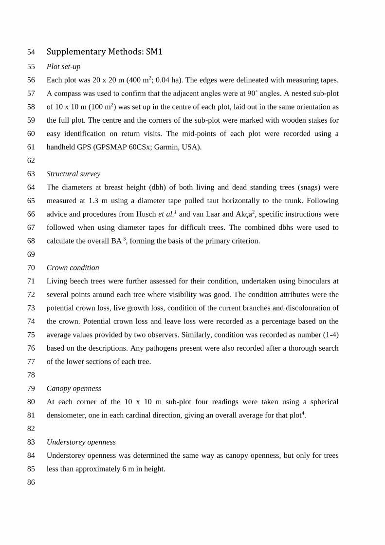
Supplementary Methods: SM1 54

Plot set-up 55

Each plot was 20 x 20 m (400 m2; 0.04 ha). The edges were delineated with measuring tapes. 56

A compass was used to confirm that the adjacent angles were at 90˚ angles. A nested sub-plot 57

of 10 x 10 m (100 m2) was set up in the centre of each plot, laid out in the same orientation as 58

the full plot. The centre and the corners of the sub-plot were marked with wooden stakes for 59

easy identification on return visits. The mid-points of each plot were recorded using a 60

handheld GPS (GPSMAP 60CSx; Garmin, USA). 61

62

Structural survey 63

The diameters at breast height (dbh) of both living and dead standing trees (snags) were 64

measured at 1.3 m using a diameter tape pulled taut horizontally to the trunk. Following 65

advice and procedures from Husch et al.1 and van Laar and Akça2, specific instructions were 66

followed when using diameter tapes for difficult trees. The combined dbhs were used to 67

calculate the overall BA 3, forming the basis of the primary criterion. 68

69

Crown condition 70

Living beech trees were further assessed for their condition, undertaken using binoculars at 71

several points around each tree where visibility was good. The condition attributes were the 72

potential crown loss, live growth loss, condition of the current branches and discolouration of 73

the crown. Potential crown loss and leave loss were recorded as a percentage based on the 74

average values provided by two observers. Similarly, condition was recorded as number (1-4) 75

based on the descriptions. Any pathogens present were also recorded after a thorough search 76

of the lower sections of each tree. 77

78

Canopy openness 79

At each corner of the 10 x 10 m sub-plot four readings were taken using a spherical 80

densiometer, one in each cardinal direction, giving an overall average for that plot4. 81

82

Understorey openness 83

Understorey openness was determined the same way as canopy openness, but only for trees 84

less than approximately 6 m in height. 85

86

Forest biomass 87

Following Jenkins et al.5, oven-dry biomass was determined in four different components of 88

the stand; the roots, the tree stems, the branches and foliage. To calculate the total biomass of 89

a single species, the stem biomass, crown biomass and root biomass were summed together 90

and multiplied by the number of that species present in the plot. The total biomass of all 91

species was then calculated by summating all individual species’ biomass values. The oven-92

dry biomass was calculated based on specific values for broadleaves, taken from McKay et 93

al6. 94

95

Carbon assessment for trees 96

Carbon content of a plot was calculated by multiplying the oven-dry matter biomass by 0.5, 97

the carbon fraction of biomass7. 98

99

Herbivore pressure metrics 100

To account for the relative presence and influence of herbivores, understorey crown 101

condition, browseline, sward height, seedling and sapling abundance, browsing intensity, 102

dung counts, and presence of a shrub layer were recorded. 103

104

For living trees in the understorey, crown condition (average of two different observers) was 105

recorded based on deviation from perceived ‘pristine’ condition (i.e. 100%). Percentage of 106

discolouration, percentage of leaves remaining, potential crown structure, empty branches 107

and position of the tree were taken into account. 108

109

The browse lines of palatable (e.g. beech, oak, birch) and unpalatable (e.g. holly, hawthorn) 110

trees were recorded if they were within the edges of the plot. Using a marked range pole, any 111

branches that were higher than 1.8 m (a deer’s maximum browse height), but lower than 2.3 112

m (based on an average drop of 50 cm in the winter), were counted as browsed. Any branches 113

that retained leaves below 1.8 m were counted as unbrowsed. A percentage ratio of browsed 114

to unbrowsed was calculated. The sward height was measured using a measuring stick, based 115

on the findings of Stewart et al.8 This was measured in the centre and at the four corners of 116

the sub-plot, and a mean value was recorded. 117

118

The percentages cover of mosses, bare ground, bracken, trampling and ground flora were 119

recorded from a detailed visual assessment of each plot. Similarly, seedling (< 1.3 m in 120

height) and sapling (> 1.3 m and dbh < 10 cm) abundances were assessed through a manual 121

search of the entire 20 x 20 m plot. Seedlings were any counted if they were older than a 122

year, based on physical aspects. 123

124

Partial defoliation or complete consumption of plants occur through herbivore browsing, the 125

intensity of which is commonly determined by counts of un-browsed and browsed 126

branches9,10. This was undertaken using a random stratified design. Initially, a 2 x 2 m 127

quadrat was placed in the most south-westerly corner of the sub-plot, continuing clockwise 128

(NW, NE, SE) around the corners, until 100 stems had been assessed. The same technique 129

was used for assessing bramble browsing, following Bazely et al 11. 130

131

For estimating herbivore abundance from dung, the faecal standing crop (FSC) method, the 132

most commonly used and efficient technique12,13, was used. A manual dung count was carried 133

out in the sub-plot; the amount, condition and the species recorded. Following Jenkins and 134

Manly14, the individual pellets/ bolus and their condition were recorded. The faecal matter of 135

different animals (deer, Equus species, rabbits and cattle) were recorded separately. 136

137

Soil survey 138

Following the methods of DeLuca et al.15, ten separate soil samples were taken in randomly-139

stratified positions, two from the centre and two at each corner of the nested 10 x 10 m sub-140

plot, for both the O horizon and A horizon soil layer (0-15 cm below the O horizon). The 141

vegetation the sample was taken under (e.g. bracken, grass) was noted. 142

143

For bulk density (BD) measurements, three 100 cm3 stainless steel rings were inserted into 144

the soil to ensure a known volume. These were taken from the SW and NE corners and from 145

the mid-point. 146

147

For analyses of NO3- and NH4

+, 5 g of sieved, field-moist soil was placed into a labelled tube 148

with 25 ml of 1 M KCl added. The soils were shaken by hand and placed horizontally on a 149

rotary shaker for 30 minutes at 250 rev/min. The extracts were immediately filtered through a 150

Fisher QT 210 filter paper into a labelled polypropylene vial. The filtrates were then frozen 151

immediately and analysed two months later. Both NH4+ and NO3

- were analysed using the 152

microplate-colorimetric technique, with the salicylate-nitroprusside method for NH4+, 153

following Mulvaney16 and the vanadium method for NO3-17. 154

155

To determine the potential mineralisable nitrogen concentrations, 5 g of sieved, field-moist 156

soil was placed into a labelled tube with 25 ml of ultrapure water added. The headspace was 157

then flushed with N2 (g). The tube was sealed and incubated for 7 days at 40°C 18. 158

Immediately after incubation, 1.75 g of KCl was added to each tube. The tubes were shaken 159

(1 hr at 200 rev/min), centrifuged and filtered immediately, using the process as for NO3- and 160

NH4+. The pH and electrical conductivity of soil was determined using a 2:1 deionized water 161

to soil ratio. 162

163

Net N mineralisation and nitrification: 164

To enable analysis of in-situ of nitrification and N mineralisation rates, following DeLuca et 165

al.15, a polyester mesh ionic resin capsule (Unibest, Walla Walla, WA, USA) was buried in 166

the centre of each plot, 10 cm deep into the mineral layer. The capsules were placed between 167

9th October and 12th November, 2014 and were removed from the ground four months later. 168

169

The nitrogen mineralisation and nitrification of a plot were analysed through leaching of resin 170

capsules (RC). Initially, 10 mL of 1 M KCl was placed into each tube containing a RC, which 171

was then shaken horizontally for 30 minutes at 250 rpm. The extractant was poured into a 172

clean storage tube. This process was repeated two more times, making a total of 30 mL of the 173

extractant. The extractant was centrifuged at 4000 rpm for 10 minutes. 20 mL of the 174

supernatant was then pipetted into a 30 mL polypropylene tube and frozen prior to 175

colorimetric analysis as described above. 176

177

Soil respiration rate: 178

Soil respiration rate was measured using a SR-1 closed chamber Infra-red gas analyser (PP 179

Systems, Amesbury, MA, USA). All measurements were recorded between 10:00 and 14:00 180

on sunny days within a month of each other. After automatic flushing and calibration of the 181

chamber, the PVC chamber was inserted 2 cm into the soil after any vegetation had been 182

removed from the surface. The CO2 concentration was measured continuously for 2 minutes. 183

Five measurements were taken from each survey plot and then averaged to produce a mean 184

soil respiration rate for the whole plot. Soil respiration rate was calculated as in (PP 185

Systems19: 186

187

R=V/A × ((Cn-Co)/(Tn )) 188

189

Where R is the respiration rate, V is the volume of the chamber, A is the area of soil exposed, 190

Cn is the CO2 concentration at time 0, and Co is the CO2 concentration at time, Tn (120 191

seconds in this study). 192

193

Soil moisture 194

Soil moisture was measured as the difference in weight of a 5 g moist soil sample before and 195

after oven-drying. Sieved mineral and organic samples were oven-dried at 105 °C and 80 °C, 196

respectively, until they remained a constant weight. To measure the soil organic matter 197

(SOM), the oven-dried samples were then placed in a 500 °C furnace overnight (12 hours), 198

the final weight recorded after being cooled in a desiccator. LOI = 100 x (mass of oven-dry 199

soil-mass of ignited soil)/ mass of oven-dry soil = g per 100g oven-dry soil20. The soil was 200

dried at 105 °C for 24 h and then sieved (2 mm) to remove stones and other non-soil material 201

(>2 mm diameter). Bulk density was calculated by dividing soil mass (less stone mass) by 202

core volume (less stone volume). 203

204

Soil content and structure 205

The Forest Research (FR) team at Alice Holt Lodge, Surrey, measured the exchangeable 206

cations/anions of K, S, Ca, Mg, Na, Al, Mn and F; total N and C, organic and inorganic C; 207

the plant-available P; and the particle sizes of the soil from air-dried samples. Following FR 208

methods, the exchangeable cations/anions were analysed using BaCl2 extraction (FR 209

Reference method: ISO 11260 & 14254). First, a soil suspension of 3 g soil and 36 ml of 0.1 210

M BaCl2 was shaken for 60 minutes, centrifuged and filtered with 0.45 µm syringe filter. 211

Extracts were then acidified and analysed using a dual view ICP-OES (Thermo ICap 6500 212

duo). The Olsen P method with ADAS index was used to determine the amount of 213

phosphorus available (FR Reference method: The analysis of Agricultural Materials MAFF 214

3rd Edition RB427). A suspension of 5 g soil with 100 ml of sodium bicarbonate solution 215

was buffered at pH 8.5. The solution was shaken for 30 min on an orbital shaker, centrifuged 216

and filtered with 0.45µm syringe filters. Extracts were then acidified with 1.5 M sulphuric 217

acid and mixed with a solution of ascorbic acid and ammonium molybdate for 10 min and 218

then measured at 880 nm with a Shimadzu UV sprectrophotometer. Total C and N were 219

analysed using a Carlo Erba CN analyser (Flash1112 series) and combustion method (FR 220

Reference method: ISO 10694 & 13878). Samples were ball-milled for homogenisation and 221

then around 30 mg weighed in tin capsules, pressed and measured using the analyser. 222

Following, 30 g of soil was placed in a silver capsule to quantify inorganic C. The silver 223

capsule was put furnace at 500oC for 2 hours, which removed the organic carbon. The 224

organic carbon fraction was calculated as the difference between total carbon and inorganic 225

carbon. The soil particle size distribution was determined using a Laser Diffraction Particle 226

Sizer (FR Reference method: Laser diffraction); 30 g of soil were suspended in water and 227

passed through the flow cell of the analyser (Beckman Coulter LS13320). 228

229

Data analysis 230

Random intercepts and slopes were included for each site. All the variables were tested for 231

normal distribution with the Shapiro–Wilk test and for homogeneity of variances for 232

Bartlett’s test21. Data that did not fit these assumptions were log-transformed prior to 233

analysis. 234

235

Count data were modelled using a Poisson error structure. For proportional and percentage 236

data, a small non-zero value was added to avoid infinite logit transformed values22. AICc 237

values were calculated using the maximum likelihood value of the model23. AICc values were 238

determined using the MuMIn R package24 and used to define the most parsimonious model, 239

following an information theoretic approach23. Performance of models was evaluated by 240

calculating the marginal r2 25. 241

Supplementary Methods: SM2 242

Ground-dwelling arthropods collection 243

Pitfall trapping was carried out in five out of the 12 sites. In each site eight pitfall traps were 244

placed on the perimeter of the 10m x 10m sub-plot; one in each corner and one midway along 245

each edge. A soil auger was used to create holes in which plastic cups (8 cm in diameter and 246

11 cm tall) were placed. Approximately 3 cm of propylene glycol, a cost effective 247

preservative, was poured into each cup. Water was allowed to escape through the use of 248

drainage holes in the top of the cups; this also prevented the trap flooding. A galvanised steel 249

square which was supported by turned-down corners was placed over each trap. Forestry 250

Commission staff collected the contents of each pitfall trap weekly from late May to late July 251

2014, totalling eight collections and 56 trapping days. The arthropod material from the eight 252

pitfall traps in each plot were pooled into a single labelled and sterilised 1 litre sample bottle 253

and then stored in -5 °C to preserve the specimens for metabarcoding. 254

255

Ground-dwelling arthropods analysis 256

DNA metabarcoding was employed for invertebrate identification using a methodology 257

tailored from the approach described in Yu et al.26. Samples were stored in absolute ethanol 258

at 4°C, followed by the extraction of DNA using the Qiagen blood and tissue extraction kit. 259

Polymerase Chain Reactions (PCR) were performed targeting the 658 base pair C terminal 260

region in the gene encoding the mitochondrial cytochrome oxidase subunit I (COI); primers 261

used for the COI region of interest were: Forward: LCO1490 (5'-262

GGTCAACAAATCATAAAGATATTGG-3') and Reverse: mlCOIintGLR (5'-GGNGGR 263

TANANNGTYCANCCNGYNCC-3'). Three separate PCRs were carried out for each 264

sample. An aliquot was checked on a 1.4% agarose gel and then the PCRs pooled before 265

library construction. A multiplex identifier (MID) tag was attached to the forward primer in 266

addition to the relevant adaptor for the sequencing platform. The MID tag was specific to 267

each sample and allowed multiple samples to be pooled for sequencing and then separated 268

out bioinformatically afterwards. A touch-down thermocycling profile was used, followed by 269

a low number of cycles with an intermediate annealing temperature. Indexing barcodes were 270

added to the amplicons following the Illumina TruSeq Nano protocol from the ‘Clean-up 271

Fragmented DNA’ stage. In a deviation from this protocol fragments were size-selected using 272

blue Pippin size selection of the 300-670bp region to remove larger fragments. The barcoded 273

samples were pooled into a single pool and 250bp paired end reads were generated on one 274

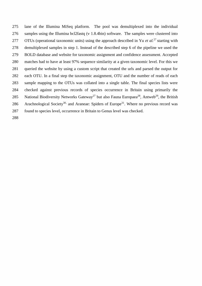
lane of the Illumina MiSeq platform. The pool was demultiplexed into the individual 275

samples using the Illumina bcl2fastq (v 1.8.4bin) software. The samples were clustered into 276

OTUs (operational taxonomic units) using the approach described in Yu et al.27 starting with 277

demultiplexed samples in step 1. Instead of the described step 6 of the pipeline we used the 278

BOLD database and website for taxonomic assignment and confidence assessment. Accepted 279

matches had to have at least 97% sequence similarity at a given taxonomic level. For this we 280

queried the website by using a custom script that created the urls and parsed the output for 281

each OTU. In a final step the taxonomic assignment, OTU and the number of reads of each 282

sample mapping to the OTUs was collated into a single table. The final species lists were 283

checked against previous records of species occurrence in Britain using primarily the 284

National Biodiversity Networks Gateway27 but also Fauna Europaea28, Antweb29, the British 285

Arachnological Society30, and Araneae: Spiders of Europe31. Where no previous record was 286

found to species level, occurrence in Britain to Genus level was checked. 287

288

Table S2: Summary of variables measured and units used. 289

Variable

Biodiversity (B), ecosystem function (EF) or ecosystem condition (EC) measure?

Units

Ectomycorrhizal fungi species richness B Unique species 0.04 ha-1

Sward height EC cm

Abundance of holly seedlings EC Individuals 0.04 ha-1

Abundance of beech seedlings EC Individuals 0.04 ha-1

Abundance of oak seedlings EC Individuals 0.04 ha-1

Abundance of tree seedlings EC Individuals 0.04 ha-1

Abundance of palatable seedlings EC Individuals 0.04 ha-1

Bulk density of the soil EC g cm-3

Depth of the organic layer EC cm

Average diameter at breast height of beech trees EC cm

Average height of beech trees EC m

Volume of standing deadwood in a plot EC m3 ha-1

Volume of lying deadwood in a plot EC m3 ha-1

C/N ratio of the soil EF C/N ratio

Potassium exchangeable cations concentration in the mineral layer soil

EF cmol(+)/kg

Magnesium exchangeable cations concentration in the mineral layer soil

EF cmol(+)/kg

Sodium exchangeable cations concentration in the mineral layer soil

EF cmol(+)/kg

Calcium exchangeable cations concentration in the mineral layer soil

EF cmol(+)/kg

Manganese exchangeable cations concentration in the mineral layer soil

EF cmol(+)/kg

Iron exchangeable cations concentration in the mineral layer soil

EF cmol(+)/kg

Aluminium exchangeable cations concentration in the mineral layer soil

EF cmol(+)/kg

Availability of soil phosphorus EF mg kg−1

Total soil nitrogen EF % of soil

Total soil carbon EF % of soil

Soil pH EF pH

Electrical conductivity EF mS m-1

Net ammonification EF µg NH4+

capsule-1 mon-1

Net nitrification EF µg NO3- capsule-1 mon-1

Net mineralisation EF µg NH4+

and NO3- capsule-1

mon-1

Soil respiration rate EF μmol m-2 s-1

Soil temperature EF °C

Total stand carbon (vegetation, deadwood and soil) EF t ha-1

Aboveground biomass EC t ha-1

Soil clay percentage EC % 0-2 µm soil particles

Soil silt percentage EC % 2-63 µm soil particles

Soil sand percentage EC % 63 µm-2 mm soil particles

Bracken cover EC % cover 0.04 ha-1

Bare ground and moss cover EC % cover 0.04 ha-1

Litter cover EC % cover 0.04 ha-1

Grass cover EC % cover 0.04 ha-1

Palatable tree browseline EC % browseline (above 1.8 m) 0.04 ha-1

Unpalatable tree browseline EC % browseline (above 1.8 m) 0.04 ha-1

Holly cover EC % cover 0.04 ha-1

Rubus cover EC % cover 0.04 ha-1

Holly shrubs browsed EC % browse of available plants

Rubus shrubs browsed EC % browse of available plants

Average crown condition EC % condition

Understorey condition EC % condition

Canopy openness EC % sky visible

Understorey openness EC % sky visible

Tree seedling richness B Unique species 0.04 ha-1

Tree sapling richness B Unique species 0.04 ha-1

Spider species richness B Unique species 0.04 ha-1

Rove beetles species richness B Unique species 0.04 ha-1

Carabid beetles species richness B Unique species 0.04 ha-1

Ant species richness B Unique species 0.04 ha-1

Weevil species richness B Unique species 0.04 ha-1

Woodlice species richness B Unique species 0.04 ha-1

Ground-dwelling arthropod species richness B Unique species 0.04 ha-1

Moisture content of the mineral layer EF % soil moisture

Moisture content of the organic layer EF % soil moisture

Cervus dung proportional EC see Jenkins and Manly (2008)

Equus dung proportional EC see Jenkins and Manly (2008)

Proportional dung total EC see Jenkins and Manly (2008)

Very large beech trees (74.97 cm < dbh < 103 cm) EC Individuals 0.04 ha-1

Large beech trees (68.32 cm < dbh < 74.97 cm) EC Individuals 0.04 ha-1

Holly tree abundance EC Individuals 0.04 ha-1

Beech trees abundance EC Individuals 0.04 ha-1

Holly saplings abundance EC Individuals 0.04 ha-1

Beech saplings abundance EC Individuals 0.04 ha-1

Overall saplings abundance EC Individuals 0.04 ha-1

Ground flora species richness B Unique species 0.04 ha-1

Woody ground flora species richness B Unique species 0.04 ha-1

Non-woody ground flora species richness B Unique species 0.04 ha-1

Lichen species richness B Unique species 0.04 ha-1

Lichen species richness on holly B Unique species 0.04 ha-1

Lichen species richness on beech B Unique species 0.04 ha-1

Organic layer loss on ignition EC % weight loss

Mineral layer loss on ignition EC % weight loss

Organic layer nitrate concentration EF mg kg−1

Mineral layer nitrate concentration EF mg kg−1

Organic layer ammonium concentration EF mg kg−1

Mineral layer ammonium concentration EF mg kg−1

Potentially mineralisable nitrogen of the organic layer EF μg g-1

Potentially mineralisable nitrogen of the mineral layer

EF μg g-1

Understorey biomass EC t ha-1

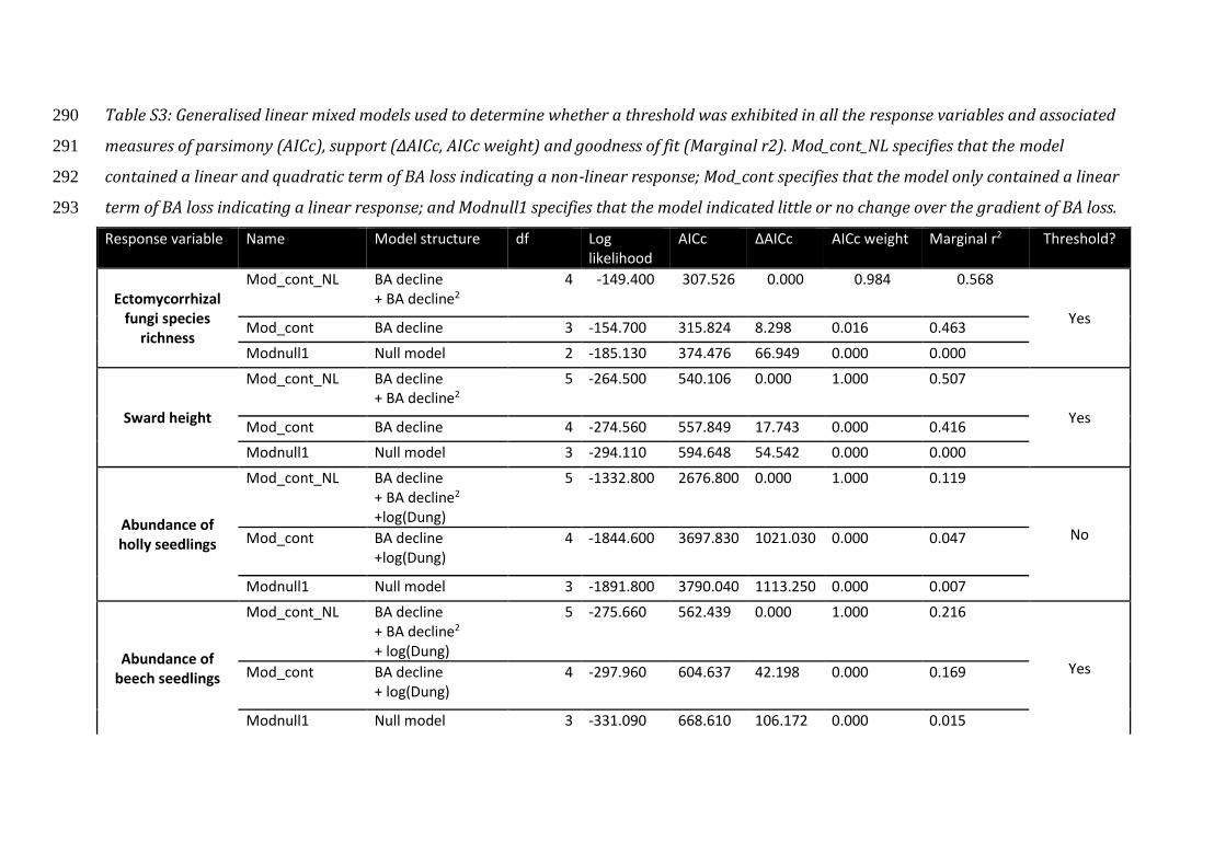
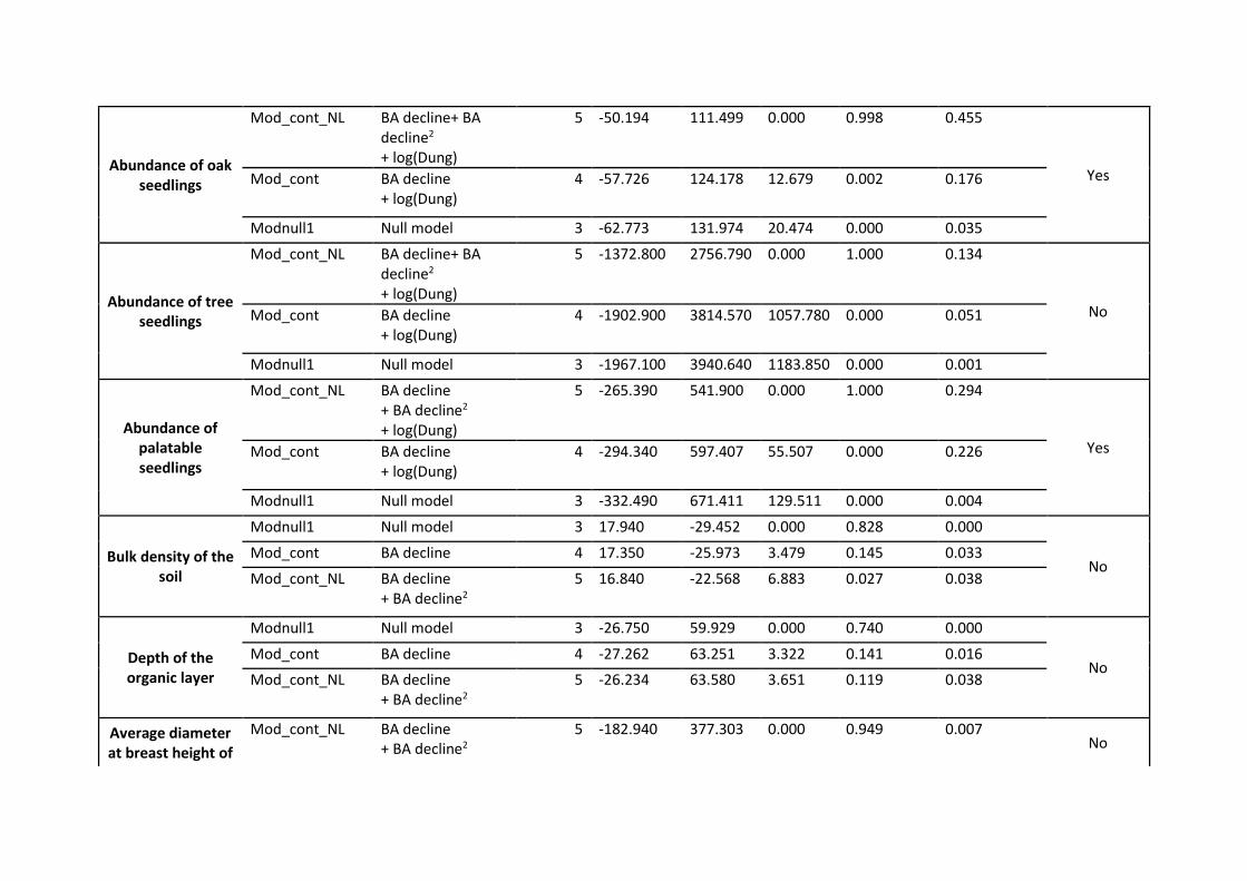
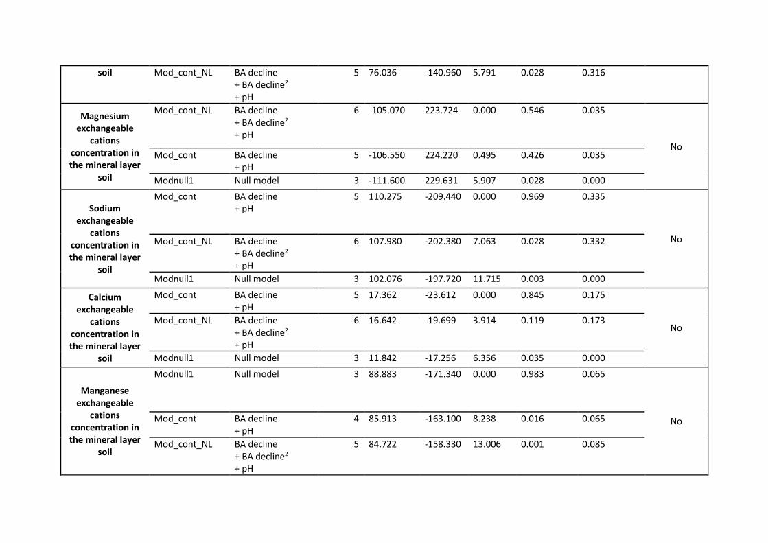
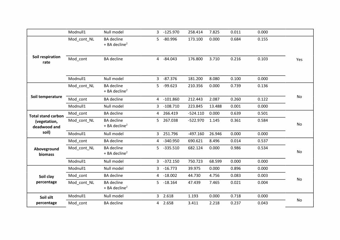
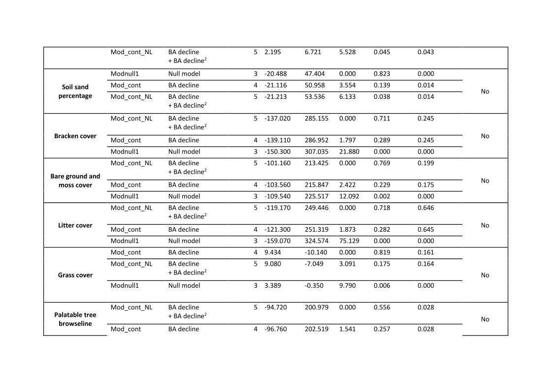
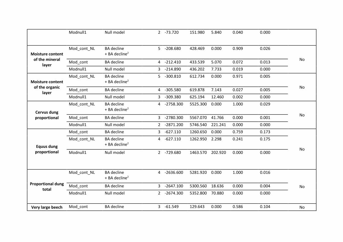
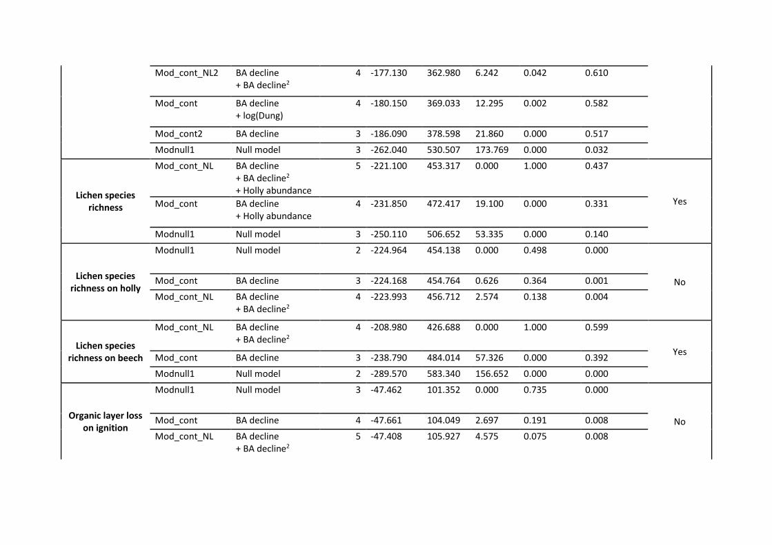
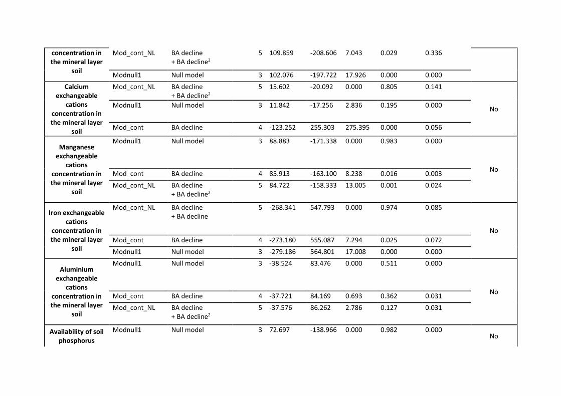
Table S3: Generalised linear mixed models used to determine whether a threshold was exhibited in all the response variables and associated 290

measures of parsimony (AICc), support (ΔAICc, AICc weight) and goodness of fit (Marginal r2). Mod_cont_NL specifies that the model 291

contained a linear and quadratic term of BA loss indicating a non-linear response; Mod_cont specifies that the model only contained a linear 292

term of BA loss indicating a linear response; and Modnull1 specifies that the model indicated little or no change over the gradient of BA loss. 293

Response variable Name Model structure df Log likelihood

AICc ΔAICc AICc weight Marginal r2 Threshold?

Ectomycorrhizal fungi species

richness

Mod_cont_NL BA decline + BA decline2

4 -149.400 307.526 0.000 0.984 0.568

Yes Mod_cont BA decline 3 -154.700 315.824 8.298 0.016 0.463

Modnull1 Null model 2 -185.130 374.476 66.949 0.000 0.000

Sward height


5 -264.500 540.106 0.000 1.000 0.507



Abundance of holly seedlings


+log(Dung)

5 -1332.800 2676.800 0.000 1.000 0.119

No Mod_cont BA decline +log(Dung)

4 -1844.600 3697.830 1021.030 0.000 0.047


Abundance of beech seedlings


+ log(Dung)

5 -275.660 562.439 0.000 1.000 0.216

Yes Mod_cont BA decline + log(Dung)

4 -297.960 604.637 42.198 0.000 0.169


Abundance of oak seedlings

Mod_cont_NL BA decline+ BA decline2

+ log(Dung)

5 -50.194 111.499 0.000 0.998 0.455


4 -57.726 124.178 12.679 0.002 0.176


Abundance of tree seedlings

Mod_cont_NL BA decline+ BA decline2 + log(Dung)

5 -1372.800 2756.790 0.000 1.000 0.134

No Mod_cont BA decline + log(Dung)

4 -1902.900 3814.570 1057.780 0.000 0.051


Abundance of palatable seedlings


+ log(Dung)

5 -265.390 541.900 0.000 1.000 0.294


4 -294.340 597.407 55.507 0.000 0.226


Bulk density of the soil

Modnull1 Null model 3 17.940 -29.452 0.000 0.828 0.000

No Mod_cont BA decline 4 17.350 -25.973 3.479 0.145 0.033


5 16.840 -22.568 6.883 0.027 0.038

Depth of the organic layer


No Mod_cont BA decline 4 -27.262 63.251 3.322 0.141 0.016


5 -26.234 63.580 3.651 0.119 0.038

Average diameter at breast height of


5 -182.940 377.303 0.000 0.949 0.007 No

beech trees Mod_cont BA decline 4 -187.300 383.531 6.228 0.042 0.003


Average height of beech trees


5 -150.090 311.599 0.000 0.907 0.046



Volume of standing

deadwood in a plot


5 -606.230 1223.580 0.000 1.000 0.043



Volume of lying deadwood in a

plot


5 -74.148 159.407 0.000 0.548 0.448



C/N ratio of the soil


+ pH

5 -154.330 319.770 0.000 0.775 0.060

No Mod_cont BA decline + pH

4 -156.800 322.325 2.555 0.216 0.056


Potassium exchangeable

cations concentration in the mineral layer


No

Mod_cont BA decline + pH

4 77.626 -146.530 0.225 0.458 0.317

soil Mod_cont_NL BA decline + BA decline2

+ pH

5 76.036 -140.960 5.791 0.028 0.316

Magnesium exchangeable


soil


+ pH

6 -105.070 223.724 0.000 0.546 0.035

No Mod_cont BA decline

+ pH 5 -106.550 224.220 0.495 0.426 0.035


Sodium exchangeable


soil


5 110.275 -209.440 0.000 0.969 0.335

No Mod_cont_NL BA decline + BA decline2

+ pH

6 107.980 -202.380 7.063 0.028 0.332


Calcium exchangeable


soil


5 17.362 -23.612 0.000 0.845 0.175

No Mod_cont_NL BA decline

+ BA decline2 + pH

6 16.642 -19.699 3.914 0.119 0.173


Manganese exchangeable


soil



4 85.913 -163.100 8.238 0.016 0.065

Mod_cont_NL BA decline + BA decline2 + pH

5 84.722 -158.330 13.006 0.001 0.085

Iron exchangeable cations

concentration in the mineral layer

soil


5 -268.340 547.793 0.000 0.974 0.085


+ pH 4 -273.180 555.087 7.294 0.025 0.072


Aluminium exchangeable


soil



4 -37.721 84.169 0.693 0.362 0.031


5 -37.576 86.262 2.786 0.127 0.031

Availability of soil phosphorus



+ pH 4 69.793 -130.860 8.108 0.017 0.000


5 68.117 -125.120 13.844 0.001 0.000

Total soil nitrogen


No


5 -62.091 135.293 6.137 0.043 0.007


6 -61.363 136.312 7.156 0.026 0.009

Total soil carbon Mod_cont_NL BA decline

+ BA decline2 + pH

6 -228.010 469.603 0.000 0.943 0.076 No


5 -232.050 475.208 5.605 0.057 0.068


Soil pH



+ BA decline2 5 -16.862 44.835 4.901 0.074 0.037

Mod_cont BA decline 4 -18.058 44.844 4.909 0.073 0.000

Electrical conductivity




5 213.517 -415.920 16.863 0.000 0.213

Net ammonification



+ BA decline2 5 -86.432 184.088 1.125 0.276 0.052


Net nitrification


5 -90.104 191.433 0.000 0.531 0.104



Net mineralisation

Mod_cont_NL2 BA decline + BA decline2 + pH

6 -118.420 250.589 0.000 0.532 0.069

No Mod_cont2 BA decline

+ pH 5 -120.620 252.466 1.877 0.208 0.064


5 -120.970 253.168 2.579 0.147 0.065



Soil respiration rate


5 -80.996 173.100 0.000 0.684 0.155



Soil temperature


5 -99.623 210.356 0.000 0.739 0.136



Total stand carbon (vegetation,

deadwood and soil)

Mod_cont BA decline 4 266.419 -524.110 0.000 0.639 0.501


+ BA decline2 5 267.038 -522.970 1.145 0.361 0.584


Aboveground biomass



+ BA decline2 5 -335.510 682.124 0.000 0.986 0.534


Soil clay percentage




5 -18.164 47.439 7.465 0.021 0.004

Soil silt percentage

Modnull1 Null model 3 2.618 1.193 0.000 0.718 0.000 No

Mod_cont BA decline 4 2.658 3.411 2.218 0.237 0.043


5 2.195 6.721 5.528 0.045 0.043

Soil sand percentage




5 -21.213 53.536 6.133 0.038 0.014

Bracken cover


5 -137.020 285.155 0.000 0.711 0.245



Bare ground and moss cover


5 -101.160 213.425 0.000 0.769 0.199



Litter cover


5 -119.170 249.446 0.000 0.718 0.646



Grass cover


No


5 9.080 -7.049 3.091 0.175 0.164


Palatable tree browseline


5 -94.720 200.979 0.000 0.556 0.028

No



Unpalatable tree browseline


5 -112.050 235.380 0.000 0.602 0.035



Holly cover



+ BA decline2 5 -64.272 140.258 0.813 0.313 0.005


Rubus cover


5 -71.326 154.366 0.000 0.622 0.184



Holly shrubs browsed




5 -56.907 124.926 0.763 0.278 0.059

Rubus shrubs browsed


5 -73.077 157.868 0.000 0.831 0.129



Average crown condition



+ BA decline2 5 9.691 -7.954 2.224 0.210 0.155


Understorey Modnull1 Null model 3 -19.867 46.350 0.000 0.829 0.000 No

condition Mod_cont BA decline 4 -20.713 50.478 4.128 0.105 0.004


5 -19.898 51.418 5.068 0.066 0.028

Canopy openness


5 -43.877 98.866 0.000 0.988 0.886



Understorey openness


5 -115.730 242.573 0.000 0.602 0.292



Tree seedling richness



+ BA decline2 4 -102.290 213.301 2.028 0.265 0.209


Tree sapling richness




4 -62.561 133.850 4.475 0.074 0.001

Spider species richness


No Modnull1 Null model 2 -57.636 119.817 1.048 0.294 0.000


4 -55.245 120.490 1.721 0.210 0.189

Rove beetles species richness


No

Mod_cont_NL BA decline 4 -48.635 107.270 1.994 0.220 0.134

+ BA decline2


Carabid beetles species richness




4 -50.590 111.179 3.573 0.103 0.086

Ant species richness


No Mod_cont_NL BA decline 4 -37.467 84.933 2.479 0.224 0.529


Weevil species richness




4 -28.165 66.330 4.719 0.068 0.048

Woodlice species richness




4 -36.943 83.887 4.857 0.065 0.029

Ground-dwelling arthropod species

richness



4 -69.280 148.560 2.410 0.220 0.283


Moisture content of the mineral

layer


5 -208.680 428.469 0.000 0.909 0.026



Moisture content of the organic

layer


5 -300.810 612.734 0.000 0.971 0.005



Cervus dung proportional


4 -2758.300 5525.300 0.000 1.000 0.029



Equus dung proportional


No


4 -627.110 1262.950 2.298 0.241 0.175


Proportional dung total


4 -2636.600 5281.920 0.000 1.000 0.016



Very large beech Mod_cont BA decline 3 -61.549 129.643 0.000 0.586 0.104 No

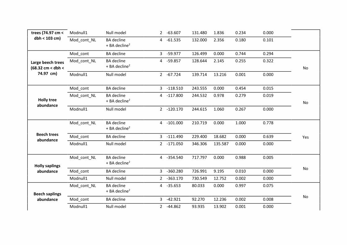
trees (74.97 cm < dbh < 103 cm)



4 -61.535 132.000 2.356 0.180 0.101

Large beech trees (68.32 cm < dbh <

74.97 cm)


No


4 -59.857 128.644 2.145 0.255 0.322


Holly tree abundance


No


4 -117.800 244.532 0.978 0.279 0.019


Beech trees abundance


4 -101.000 210.719 0.000 1.000 0.778



Holly saplings abundance


4 -354.540 717.797 0.000 0.988 0.005



Beech saplings abundance


4 -35.653 80.033 0.000 0.997 0.075



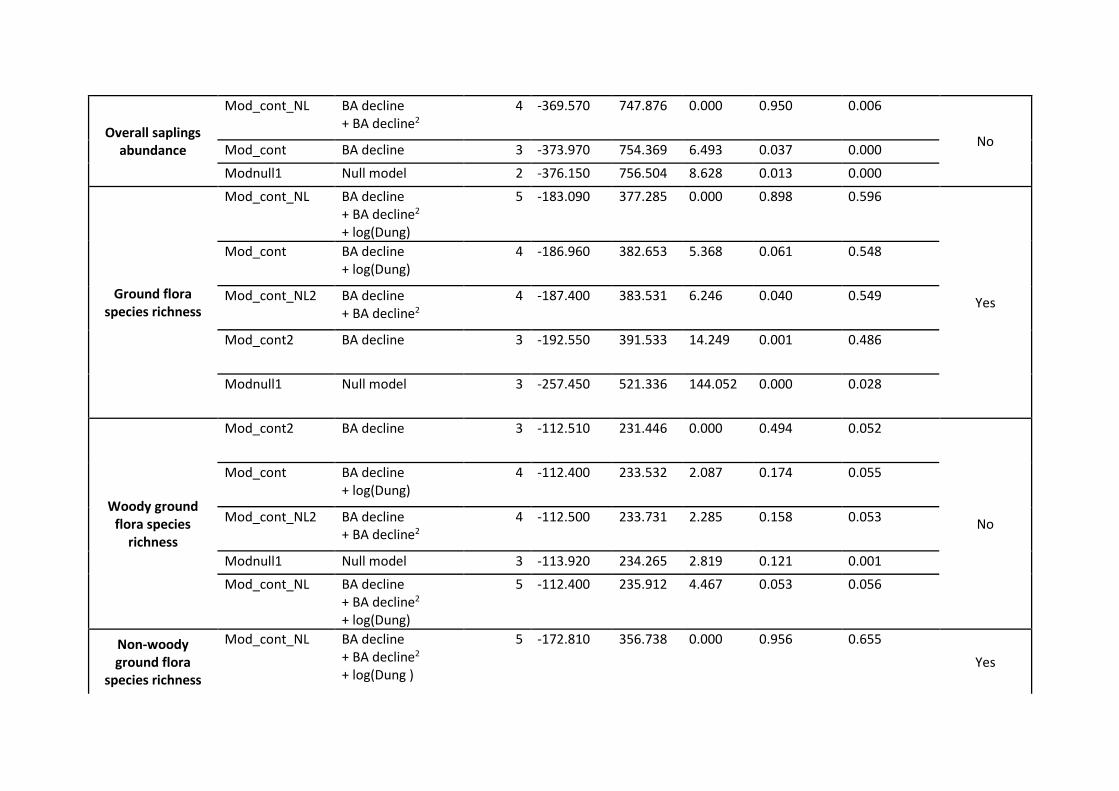
Overall saplings abundance


4 -369.570 747.876 0.000 0.950 0.006



Ground flora species richness


+ log(Dung)

5 -183.090 377.285 0.000 0.898 0.596

Yes

Mod_cont BA decline + log(Dung)

4 -186.960 382.653 5.368 0.061 0.548

Mod_cont_NL2 BA decline + BA decline2

4 -187.400 383.531 6.246 0.040 0.549

Mod_cont2 BA decline 3 -192.550 391.533 14.249 0.001 0.486


Woody ground flora species

richness


No


4 -112.400 233.532 2.087 0.174 0.055


4 -112.500 233.731 2.285 0.158 0.053


Mod_cont_NL BA decline + BA decline2 + log(Dung)

5 -112.400 235.912 4.467 0.053 0.056

Non-woody ground flora

species richness

Mod_cont_NL BA decline + BA decline2 + log(Dung )

5 -172.810 356.738 0.000 0.956 0.655

Yes


4 -177.130 362.980 6.242 0.042 0.610


4 -180.150 369.033 12.295 0.002 0.582



Lichen species richness

Mod_cont_NL BA decline + BA decline2 + Holly abundance

5 -221.100 453.317 0.000 1.000 0.437

Yes Mod_cont BA decline + Holly abundance

4 -231.850 472.417 19.100 0.000 0.331


Lichen species richness on holly




4 -223.993 456.712 2.574 0.138 0.004

Lichen species richness on beech


4 -208.980 426.688 0.000 1.000 0.599



Organic layer loss on ignition




5 -47.408 105.927 4.575 0.075 0.008

Mineral layer loss on ignition




5 -62.180 135.470 2.271 0.167 0.020

Organic layer nitrate

concentration



5 -60.917 132.946 0.335 0.338 0.054


Mineral layer nitrate

concentration



5 -60.917 132.946 0.335 0.338 0.054


Organic layer ammonium

concentration


5 -235.070 481.246 0.000 0.959 0.052



Mineral layer ammonium

concentration




5 -43.620 98.351 4.361 0.088 0.006

Potentially mineralisable

nitrogen of the organic layer



+ BA decline2 5 -120.250 251.611 0.702 0.325 0.001



nitrogen of the mineral layer

Mod_cont_NL BA decline + BA decline2 + soil moisture

6 -186.840 387.270 0.000 0.974 0.129


+ soil moisture 5 -191.740 394.586 7.317 0.025 0.091


Understorey biomass


6 -137.210 288.010 0.000 0.905 0.380



294

Table S4: Updated version of Table S3 with only linear and quadratic term of BA included as fixed effects. 295

Response variable Name Model structure df Log likelihood

AICc ΔAICc AICc weight Marginal r2 Threshold?

Abundance of holly seedlings


4 -1364.378 2737.483 0.000 1.000 0.116



Abundance of beech seedlings


4 -279.394 567.515 0.000 1.000 0.217



Abundance of oak seedlings


4 -50.284 109.295 0.000 0.999 0.444



Abundance of tree seedlings


4 -1403.461 2815.650 0.000 1.000 0.134



Abundance of palatable


4 -267.337 543.401 0.000 1.000 0.293 Yes

seedlings Mod_cont BA decline 3 -296.268 598.964 55.564 0.000 0.224




C/N ratio of the soil


5 -154.329 319.770 0.000 0.775 0.060



Potassium exchangeable


soil



Mod_cont_NL BA decline + BA decline

5 76.035 -140.960 5.791 0.028 0.102

Magnesium exchangeable


soil


5 -109.120 229.352 0.000 0.380 0.018

No



Sodium exchangeable

cations


No


soil


5 109.859 -208.606 7.043 0.029 0.336


Calcium exchangeable


soil


5 15.602 -20.092 0.000 0.805 0.141

No Modnull1 Null model 3 11.842 -17.256 2.836 0.195 0.000


Manganese exchangeable


soil




5 84.722 -158.333 13.005 0.001 0.024

Iron exchangeable cations


soil

Mod_cont_NL BA decline + BA decline

5 -268.341 547.793 0.000 0.974 0.085

No



Aluminium exchangeable


soil




5 -37.576 86.262 2.786 0.127 0.031

Availability of soil phosphorus

Modnull1 Null model 3 72.697 -138.966 0.000 0.982 0.000 No



5 68.117 -125.122 13.844 0.001 0.000

Total soil nitrogen




5 -61.260 133.631 4.475 0.083 0.003

Total soil carbon


5 -230.653 472.418 0.000 0.943 0.077



Net mineralisation


5 -120.972 253.168 0.000 0.706 0.065



Ground flora species richness


4 -187.402 383.531 0.000 0.982 0.549



Woody ground flora species

richness


No Modnull1 Null model 2 -113.948 232.107 0.662 0.353 0.000


4 -112.502 233.731 2.285 0.157 0.053

Non-woody ground flora

species richness


4 -177.126 362.979 0.000 1.000 0.610

Yes

Mod_cont BA decline + BA decline2

3 -186.085 378.598 15.618 0.000 0.517

Modnull1 BA decline 2 -262.197 528.604 165.624 0.000 0.000

Lichen species richness


4 -243.059 494.845 0.000 0.998 0.240




nitrogen of the mineral layer


5 -185.964 383.038 0.000 0.982 0.114



296

297

298

Table S5: Statistics of the soil properties. Mean, standard deviation (SD), standard error (SE), and confidence interval (CI) of several soil 299

properties across the stages of dieback. 300

Percent

basal area

decline N Mean SD SE CI

Clay (%)

0% 12 20.42 3.68 1.06 2.34

25% 12 20.00 4.75 1.37 3.02

50% 12 21.08 7.29 2.11 4.63

75% 12 19.08 6.24 1.80 3.97

100% 12 20.58 7.90 2.28 5.02

Sand (%)

0% 12 48.83 6.79 1.96 4.32

25% 12 49.50 6.47 1.87 4.11

50% 12 49.50 10.12 2.92 6.43

75% 12 52.50 10.98 3.17 6.97

100% 12 51.08 10.40 3.00 6.61

Silt (%)

0% 12 30.75 4.81 1.39 3.05

25% 12 30.50 4.52 1.31 2.87

50% 12 29.42 4.87 1.41 3.09

75% 12 28.42 5.68 1.64 3.61

100% 12 28.33 4.21 1.21 2.67

pH

0% 12 4.19 0.28 0.08 0.18

25% 12 4.40 0.38 0.11 0.24

50% 12 4.37 0.28 0.08 0.18

75% 12 4.27 0.27 0.08 0.17

100% 12 4.27 0.35 0.10 0.23

Moisture content (Organic layer)

0% 12 157.07 41.05 11.85 26.08

25% 12 163.33 50.04 14.45 31.80

50% 12 149.21 53.35 15.40 33.89

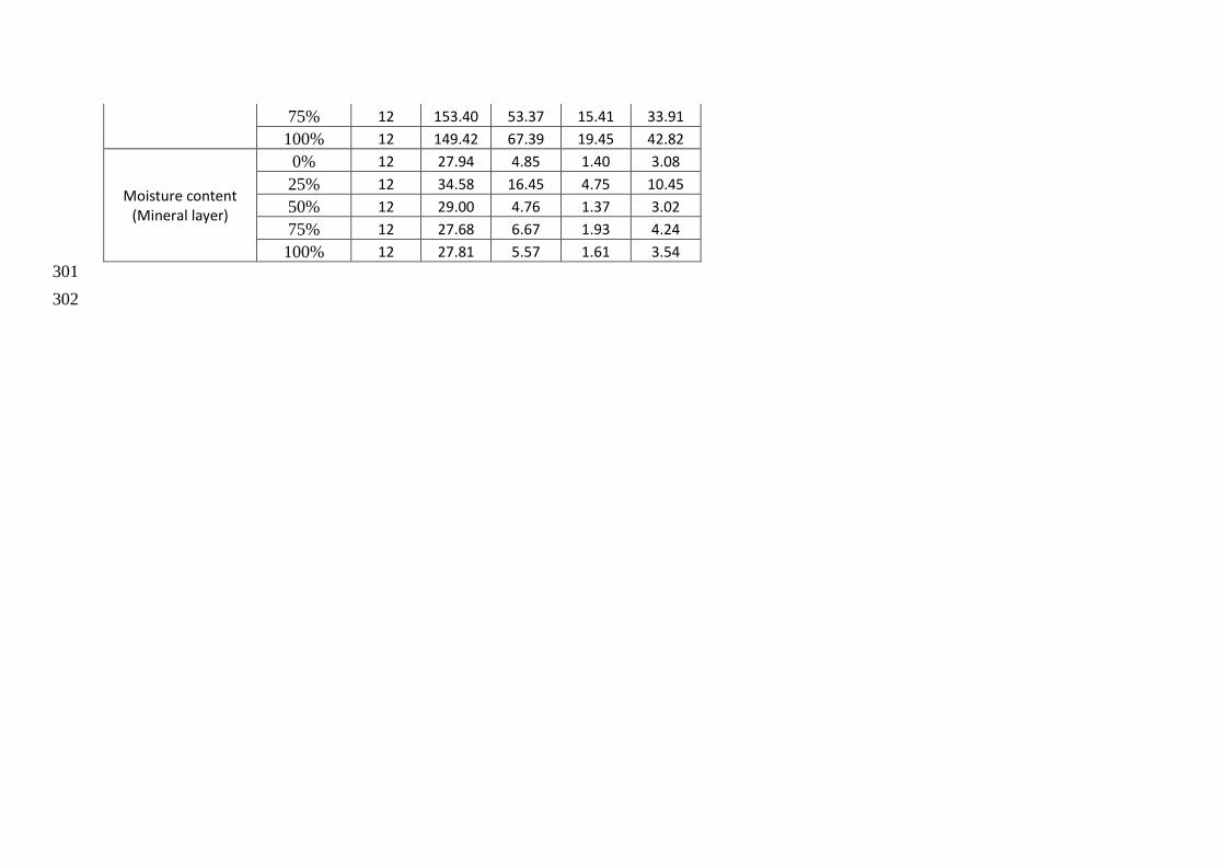
75% 12 153.40 53.37 15.41 33.91

100% 12 149.42 67.39 19.45 42.82

Moisture content (Mineral layer)

0% 12 27.94 4.85 1.40 3.08

25% 12 34.58 16.45 4.75 10.45

50% 12 29.00 4.76 1.37 3.02

75% 12 27.68 6.67 1.93 4.24

100% 12 27.81 5.57 1.61 3.54

301

302

Supplementary Methods: SM3. Graphs to support the space-for-time 303

assumption 304

305

306

Fig S3: Mean values (n = 12) of a) clay soil content; b) depth of the organic soil layer; c) pH of the soil across 307

the gradient of dieback; and d) diameter at breast height (DBH) of the living beech trees across the gradient 308

of dieback. The black bars indicate the standard error of the mean. 309

310

311

312

313

Fig S4: Mean values of a) the total herbivore dung count, and b) percentage of holly shoots browsed by 314

herbivores across the gradient of dieback. The black bars indicate the standard error of the mean. 315

316

Supplementary references 317

1. Husch, B., Beers, T. W. & Kershaw, J. A. Forest mensuration (Wiley, 2003). 318

2. van Laar, A. & Akça, A. Forest mensuration (Springer, 2007). 319

3. Cantarello, E. & Newton, A. C. Identifying cost-effective indicators to assess the 320

conservation status of forested habitats in Natura 2000 sites. For. Ecol. Manage. 256, 321

815-826, doi:10.1016/j.foreco.2008.05.031 (2008). 322

4. Strickler, G. S. Use of the densiometer to estimate density of forest canopy on 323

permanent sample plots (USDA Forest Service, 1959). 324

5. Jenkins, T. A. R. et al. FC woodland carbon code: Carbon assessment protocol 325

(Forestry Commission, 2011). 326

6. McKay, H., Hudson, J. B. & Hudson, R. J. Woodfuel resource in Britain: Appendices. 327

Fes b/w3/00787/rep/2. Dti/pub urn 03/1436 (Forestry Contracting Association, 2003). 328

7. Matthews, G. A. R. The carbon content of trees. Forestry commission technical paper 329

4 (Forestry Commission, 1993). 330

8. Stewart, K. E. J., Bourn, N. A. D. & Thomas, J. A. An evaluation of three quick 331

methods commonly used to assess sward height in ecology. J. Appl. Ecol. 38, 1148-332

1154, doi:10.1046/j.1365-2664.2001.00658.x (2001). 333

9. Bergström, R. & Guillet, C. Summer browsing by large herbivores in short-rotation 334

willow plantations. Biomass Bioenergy 23, 27-32, doi:10.1016/S0961-335

9534(02)00027-2 (2002). 336

10. Gibson, D. J. Methods in comparative plant population ecology (Oxford University 337

Press, 2002). 338

11. Bazely, D. R., Myers, J. H. & da Silva, K. B. The response of numbers of bramble 339

prickles to herbivory and depressed resource availability. Oikos 61, 327-336, 340

doi:10.2307/3545240 (1991). 341

12. Campbell, D., Swanson, G. M. & Sales, J. Methodological insights: Comparing the 342

precision and cost-effectiveness of faecal pellet group count methods. J. Appl. Ecol. 343

41, 1185-1196, doi:10.1111/j.0021-8901.2004.00964.x (2004). 344

13. Marques, F. F. C. et al. Estimating deer abundance from line transect surveys of dung: 345

Sika deer in southern Scotland. J. Appl. Ecol.38, 349-363, doi:10.1046/j.1365-346

2664.2001.00584.x (2001). 347

14. Jenkins, K. J. & Manly, B. A double‐observer method for reducing bias in faecal 348

pellet surveys of forest ungulates. J. Appl. Ecol.45, 1339-1348, doi:10.1111/j.1365-349

2664.2008.01512.x (2008). 350

15. DeLuca, T., Zewdie, S., Zackrisson, O., Healey, J. & Jones, D. Bracken fern 351

(Pteridium aquilinum L. Kuhn) promotes an open nitrogen cycle in heathland soils. 352

Plant Soil 367, 521-534, doi:10.1007/s11104-012-1484-0 (2013). 353

16. Mulvaney, R. S. Nitrogen - inorganic forms in Methods of soil analysis. Part 3 - 354

chemical methods (ed. Sparks, D. L.) 1123–1184 (Soil Science Society of America, 355

1996). 356

17. Miranda, K. M., Espey, M. G. & Wink, D. A. A rapid, simple spectrophotometric 357

method for simultaneous detection of nitrate and nitrite. Nitric Oxide 5, 62-71, 358

doi:10.1006/niox.2000.0319 (2001). 359

18. Keeney, D. R. in Methods of soil analysis: Chemical and microbiological properties 360

(eds. Page, A. L., Miller, R. H. & Keeney, D. R.) (Soil Society of America, 1982). 361

19. PP Systems. EGM-4 Environmental Gas Monitor for CO2: Operator's manual version 362

4.18 (PP Systems, 2010). 363

20. Rowell, D. L. Soil science: Methods & application (John Wiley & Sons, Ltd, 1994). 364

21. Dytham, C. Choosing and using statistics: A biologist's guide (John Wiley & Sons, 365

2011). 366

22. Warton, D. I. & Hui, F. K. C. The arcsine is asinine: The analysis of proportions in 367

ecology. Ecology 92, 3-10, doi:10.1890/10-0340.1 (2010). 368

23. Burnham, K. P. & Anderson, D. R. Model selection and multimodel inference 369

(Springer-Verlag, 2002). 370

24. Barton, K. Mumin: Multi-model inference: R package version 1.10.0. (2014). 371

25. Nakagawa, S. & Schielzeth, H. A general and simple method for obtaining R2 from 372

generalized linear mixed‐effects models. Methods Ecol. Evol. 4, 133-142 (2013). 373

26. Yu, D. W. et al. Biodiversity soup: Metabarcoding of arthropods for rapid 374

biodiversity assessment and biomonitoring. Methods Ecol. Evol. 3, 613-623, 375

doi:10.1111/j.2041-210X.2012.00198.x (2012). 376

27. NBN Gateway. National Biodiversity Networks Gateway https://data.nbn.org.uk/ 377

(2015). 378

28. de Jong, Y. et al. Fauna Europaea – all European animal species on the web. 379

Biodiversity Data Journal. 2, e4034, doi:10.3897/BDJ.2.e4034 (2014). 380

29. AntWeb. AntWeb https://www.antweb.org (2015) 381

30. British Arachnological Society. Spider and harvestman recording scheme 382

http://srs.britishspiders.org.uk (2015). 383

31. Nentwig W, Blick T, Gloor D, Hänggi A, Kropf C. Spiders of Europe 384

www.araneae.unibe.ch (2015). 385

386

6 P. M. Evans 1 2 3 7 Barsoum 10 11 SO40 7HU, UK. 12 13 ...10.1038/s41598-017... · 7 Barsoum 4, J....

Documents

Transcript of 6 P. M. Evans 1 2 3 7 Barsoum 10 11 SO40 7HU, UK. 12 13 ...10.1038/s41598-017... · 7 Barsoum 4, J....