6: Neyman-Pearson DetectorsECE 830, Spring 2014

1 / 21

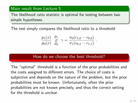
Main result from Lecture 5

The likelihood ratio statistic is optimal for testing between twosimple hypotheses.

The test simply compares the likelihood ratio to a threshold:

p1(x)

p0(x)

H1

≷H0

γ =π0(c1,0 − c0,0)π1(c0,1 − c1,1)

.

How do we choose the best threshold?

The “optimal” threshold is a function of the prior probabilities andthe costs assigned to different errors. The choice of costs issubjective and depends on the nature of the problem, but the priorprobabilities must be known. Unfortunately, often the priorprobabilities are not known precisely, and thus the correct settingfor the threshold is unclear.

2 / 21

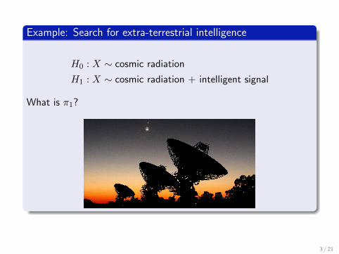
Example: Search for extra-terrestrial intelligence

H0 : X ∼ cosmic radiation

H1 : X ∼ cosmic radiation + intelligent signal

What is π1?

3 / 21

Alternative design specification

Let’s design a test that minimizes one type of error subject to aconstraint on the other type of error.

This constrained optimization criterion does not require knowledgeof prior probabilities or cost assignments. It only requires aspecification of the maximum allowable value for one type of error,which is sometimes even more natural than assigning costs to thedifferent errors.

Neyman Pearson testing

A classic result due to Neyman and Pearson shows that thesolution to this type of optimization is again a likelihood ratio test.

4 / 21

Neyman-Pearson LemmaAssume that we observe a random variable distributed according toone of two distributions.

H0 : X ∼ p0

H1 : X ∼ p1

Definition: null and alternative hypotheses

H0 is consider to be a sort of baseline or default model and iscalled the null hypothesis. H1 is a different model and is called thealternative hypothesis.

Definition: false alarms and misses

If a test chooses H1 when in fact the data were generated by H0

the error is called a false-positive or false-alarm, since wemistakenly accepted the alternative hypothesis. The error ofdeciding H0 when H1 was the correct model is called afalse-negative or miss.

5 / 21

Let T denote a testing procedure based on an observation of X.and let RT denote the subset of the range of X where the testchooses H1. The probability of a false-positive is denoted by

PFA = P0(RT ) :=

∫RT

p0(x) dx .

The probability of a false-negative is PM = 1− P1(RT ), where

PD = P1(RT ) :=

∫RT

p1(x) dx ,

is the probability of correctly deciding H1, often called theprobability of detection.

Note that PFA and PD do not depend on prior probabilities π0and π1.

6 / 21

Statistics vocabulary

These same ideas all arise in statistics, but that community usesdifferent language.

I 1− PFA is call the specificity of a test.

I PD = 1− PM is called the power or sensitivity of a test.

I Engineers talk about keeping PFA small while maximizing PD.

I Statisticians talk about keeping both the specificity and powerof a test large.

I These are equivalent ideas.

7 / 21

Consider likelihood ratio tests of the form

p1(x)

p0(x)

H1

≷H0

λ .

The subset of the range of X where this test decides H1 is denoted

RLR(λ) := {x : p1(x) > λp0(x)} ,

and therefore the probability of a false-positive decision is

P0(RLR(λ)) :=

∫RLR(λ)

p0(x) dx =

∫{x:p1(x)>λp0(x)}

p0(x) dx

This probability is a function of the threshold λ; the set RLR(λ)shrinks/grows as λ increases/decreases. We can select λ toachieve a desired probability of error.

8 / 21

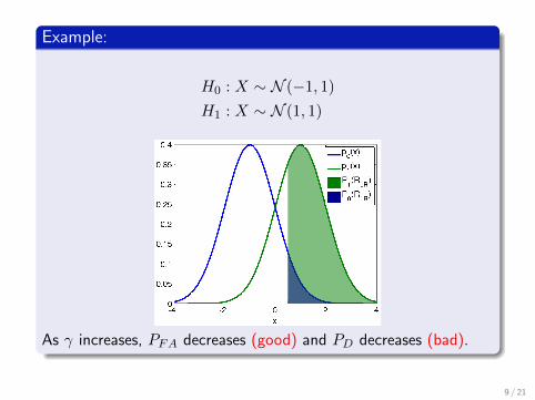
Example:

H0 : X ∼ N (−1, 1)H1 : X ∼ N (1, 1)

As γ increases, PFA decreases (good) and PD decreases (bad).

9 / 21

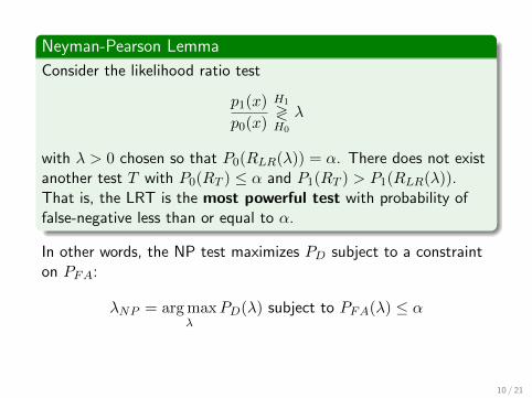
Neyman-Pearson Lemma

Consider the likelihood ratio test

p1(x)

p0(x)

H1

≷H0

λ

with λ > 0 chosen so that P0(RLR(λ)) = α. There does not existanother test T with P0(RT ) ≤ α and P1(RT ) > P1(RLR(λ)).That is, the LRT is the most powerful test with probability offalse-negative less than or equal to α.

In other words, the NP test maximizes PD subject to a constrainton PFA:

λNP = argmaxλ

PD(λ) subject to PFA(λ) ≤ α

10 / 21

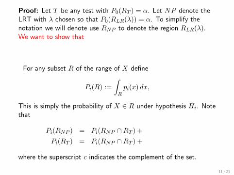
Proof: Let T be any test with P0(RT ) = α. Let NP denote theLRT with λ chosen so that P0(RLR(λ)) = α. To simplify thenotation we will denote use RNP to denote the region RLR(λ).We want to show that

P1(RT ) ≤ P1(RNP ).

For any subset R of the range of X define

Pi(R) :=

∫Rpi(x) dx,

This is simply the probability of X ∈ R under hypothesis Hi. Notethat

Pi(RNP ) = Pi(RNP ∩RT ) +

Pi(RNP ∩RcT )

Pi(RT ) = Pi(RNP ∩RT ) +

Pi(RcNP ∩RT )

where the superscript c indicates the complement of the set.

11 / 21

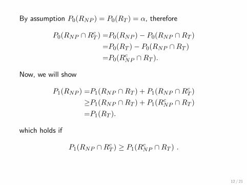
By assumption P0(RNP ) = P0(RT ) = α, therefore

P0(RNP ∩RcT ) =P0(RNP )− P0(RNP ∩RT )=P0(RT )− P0(RNP ∩RT )=P0(R

cNP ∩RT ).

Now, we will show

P1(RNP ) =P1(RNP ∩RT ) + P1(RNP ∩RcT )≥P1(RNP ∩RT ) + P1(R

cNP ∩RT )

=P1(RT ).

which holds if

P1(RNP ∩RcT ) ≥ P1(RcNP ∩RT ) .

12 / 21

To see that this is indeed the case,

P1(RNP ∩RcT ) =

∫RNP∩RcT

p1(x) dx

≥ λ

∫RNP∩RcT

p0(x) dx

= λ p0(RNP ∩RcT )= λ p0(R

cNP ∩RT )

= λ

∫RcNP∩RT

p0(x) dx

≥∫RcNP∩RT

p1(x) dx

= P1(RcNP ∩RT ).

13 / 21

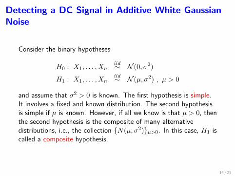
Detecting a DC Signal in Additive White GaussianNoise

Consider the binary hypotheses

H0 : X1, . . . , Xniid∼ N (0, σ2)

H1 : X1, . . . , Xniid∼ N (µ, σ2) , µ > 0

and assume that σ2 > 0 is known. The first hypothesis is simple.It involves a fixed and known distribution. The second hypothesisis simple if µ is known. However, if all we know is that µ > 0, thenthe second hypothesis is the composite of many alternativedistributions, i.e., the collection {N(µ, σ2)}µ>0. In this case, H1 iscalled a composite hypothesis.

14 / 21

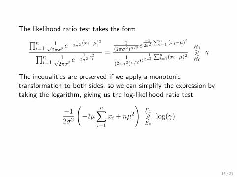
The likelihood ratio test takes the form∏ni=1

1√2πσ2

e−1

2σ2(xi−µ)2∏n

i=11√2πσ2

e−1

2σ2x2i

=

1(2πσ2)n/2

e−1

2σ2

∑ni=1 (xi−µ)2

1(2πσ2)n/2

e−1

2σ2

∑ni=1(xi−µ)2

H1

≷H0

γ

The inequalities are preserved if we apply a monotonictransformation to both sides, so we can simplify the expression bytaking the logarithm, giving us the log-likelihood ratio test

−12σ2

(−2µ

n∑i=1

xi + nµ2

)H1

≷H0

log(γ)

15 / 21

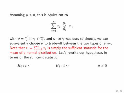
Assuming µ > 0, this is equivalent to

n∑i=1

xiH1

≷H0

ν ,

with ν = σ2

µ ln γ + nµ2 , and since γ was ours to choose, we can

equivalently choose ν to trade-off between the two types of error.Note that t :=

∑ni=1 xi is simply the sufficient statastic for the

mean of a normal distribution. Let’s rewrite our hypotheses interms of the sufficient statistic:

H0 : t ∼

N (0, nσ2),

H1 : t ∼

N (nµ, nσ2),

µ > 0

16 / 21

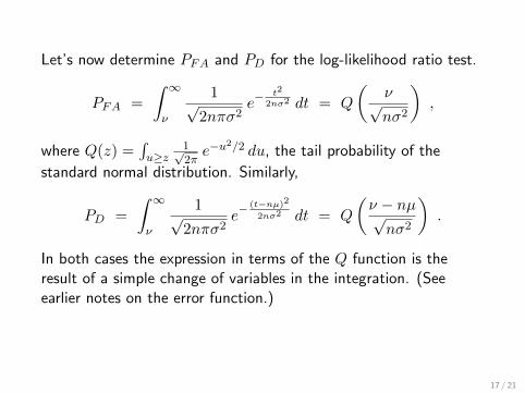
Let’s now determine PFA and PD for the log-likelihood ratio test.

PFA =

∫ ∞ν

1√2nπσ2

e−t2

2nσ2 dt = Q

(ν√nσ2

),

where Q(z) =∫u≥z

1√2πe−u

2/2 du, the tail probability of the

standard normal distribution. Similarly,

PD =

∫ ∞ν

1√2nπσ2

e−(t−nµ)2

2nσ2 dt = Q

(ν − nµ√nσ2

).

In both cases the expression in terms of the Q function is theresult of a simple change of variables in the integration. (Seeearlier notes on the error function.)

17 / 21

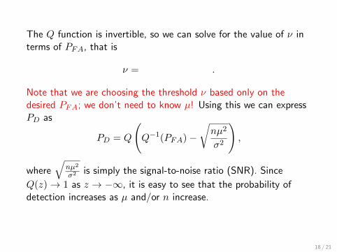
The Q function is invertible, so we can solve for the value of ν interms of PFA, that is

ν =

√nσ2Q−1(PFA)

.

Note that we are choosing the threshold ν based only on thedesired PFA; we don’t need to know µ! Using this we can expressPD as

PD = Q

(Q−1(PFA)−

√nµ2

σ2

),

where√

nµ2

σ2 is simply the signal-to-noise ratio (SNR). Since

Q(z)→ 1 as z → −∞, it is easy to see that the probability ofdetection increases as µ and/or n increase.

18 / 21

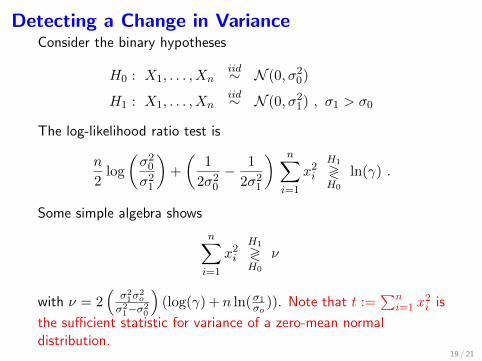
Detecting a Change in VarianceConsider the binary hypotheses

H0 : X1, . . . , Xniid∼ N (0, σ20)

H1 : X1, . . . , Xniid∼ N (0, σ21) , σ1 > σ0

The log-likelihood ratio test is

n

2log

(σ20σ21

)+

(1

2σ20− 1

2σ21

) n∑i=1

x2iH1

≷H0

ln(γ) .

Some simple algebra shows

n∑i=1

x2iH1

≷H0

ν

with ν = 2(σ21σ

2o

σ21−σ2

0

)(log(γ) + n ln(σ1σo )). Note that t :=

∑ni=1 x

2i is

the sufficient statistic for variance of a zero-mean normaldistribution.

19 / 21

Now recall that if X1, . . . , Xniid∼ N(0, 1), then

∑ni=1X

2i ∼ χ2

n

(chi-square distributed with n degrees of freedom). Let’s rewriteour null hypothesis test using the sufficient statistic:

H0 : t =

n∑i=1

x2iσ20∼ χ2

n

The probability of false alarm is just the probability that a χ2n

random variable exceeds ν/σ20. This can be easily computednumerically. For example, if we have n = 20 and set PFA = 0.01,then the correct threshold is ν = 37.57σ20.

20 / 21

Applying the NP test

1. Decide which hypothesis to call the null and which to call thealternative. Usually we choose for the null the hypothesiswhere we have more serious consequences if it’s rejected(because with NP testing we control the probability ofrejecting the null).

2. Select the power of the test. Often we see α = 0.05, meaningwe will accept a 5% chance of falsely rejecting the null (e.g.,falsely saying a target is present when it is not).

3. Use the likelihood ratio and α to choose the threshold level ν.Often this can be made simpler by expressing the problem interms of sufficient statistics.

21 / 21