6-GHZ Digital Systems Radio Engineering Microwave...

AT&T WESTERNELECTRICPRACTICESStandard

SECTION 940-300-130Issue2, March 1984

6-GHZ DIGITAL SYSTEMS

RADIO ENGINEERING

MICROWAVE RADIO

CONTENTS PAGE

1. INTRODUCTION . . . . . . . . . . . . . . . . . ...”” ““”.””””

A. General . . . . . . . . . . . . . . . . . . . . . . . ........

B. Digital Advantage . . . . . . . . . . . . . . . . . . . . . . . . . . .

c. Further Characteristics . . . . . . . . . . . . . . . . . . . . . . . . . .

2. KC RULESAND GENERALGUIDELINES . . . . . . . . . . . . . . . . . . . . . .

A. FCC Rules . . . . . . . . . . . . . . . . . . . . . . . . . . . . . .

B. Equipment Characteristicsand Requirements . . . . . . . . . . . . . . . . . .

c. Distanceand loading Rules... . . . . . . . . . . . . . . . . . . . . .

D. Checkof Modulation and FrequencyCharacteristics . . . . . . . . . . . . . . . .

E. Additional Guidelines . . . . . . . . . . . . . . . . . . . . . . . . . .

3. SYSTEMCHARACTERISTICSAND OVERVIEW . . . . . . . . . . . . . . . . . . . .

A.

B.

c.

D.

E.

F.

G.

H.

1.

General . . ..”...... . . . . . . . . . . .

TheoreticalFade Margin . . . . . . . . . . . . . . .

Fade Margin ReductionsCaused by Interferenceand LXspersiveFading

Interference . . . . . . . . . . . . . . . . . . .

Bit ErrorRate(BER) . . . . . . . . . . . . . . . . .

Modulation Types . . . . . . . . . . . . . . . . .

RepeaterTypes . . . . . . . . . . . . ...’...

Auxiliary Channels . . . . . . . . . . . . . . . . .

Maintenance Considerations . . . . . . . . . . . . . .

NOTICE

Not for use or disclosure outside the

AT&T Companies except under written agreement

Printed in U.S.A.

. . . . . . . . . .

. . . . . . . . . .

. . . . . . . . .

. . . . . . . . . .

. . . . . . . . . .

. . . . . . . . . .

. . . . . . . . . .

. . . . . . . . . .

. . . . . . . . . .

4

4

4

4

5

5

5

8

9

9

12

12

12

15

16

16

18

18

18

19

SECTION940-300-130

CONTENTS

4. RELIABILITY . . . . .

A. General . . . . .

B. Digital O~ective . .

c. Causesof Outage .

D. Dkersity Protection .

. .

. .

. .

. .

. .

E. Paths With Ground Reflections

F. Terrain Clearance . . . .

5. OUTAGE OBJKTIVES ~ . . . . .

A. General . . . . . . . .

B. HistoricalOb~tive . . . .

.

.

.

.

.

.

.

c. long-Haul Versus Short-Haul Systems

D. Maximum Length of Short-Haul Radio Systems

.

.

.

.

.

.

.

.

.

.

.

.

.

.

.

.

.

.

.

.

.

.

.

.

.

.

E. Route Design to Standards Tighter Than Short Haul

6. DISPERSIONOUTAGE . . . . . . . . . . . .

A. General . . . . . . . . . . . . . . .

B. Dispersion . . . . . . . . . . . . . .

c. Estimationof Outage . . . . . . . . . .

D. Outage calculation . . . . . . . . . . .

E. Spce-Dwersity Improvement . . . . . . . .

F. Summary Examples . . . . . . . . . . .

7. OUTAGE DUE TO EQUIPMENT FAILURE . . . . . .

A. General . . . . . . . . . . . . . . .

B. Outages Due to Double Equipment Failures . . .

.

.

.

.

.

.

.

.

.

.

.

.

.

.

.

.

.

.

.

.

.

.

.

.

.

.

.

.

.

.

.

.

.

.

.

.

.

.

.

.

.

.

.

.

.

.

.

.

.

.

.

.

.

.

.

.

.

.

.

.

.

.

.

.

.

.

.

.

.

.

.

.

.

.

.

.

.

.

.

.

.

.

c. Outage; Due to Joint Equipment and ProtectionSwitching System Failure

8. INTERFERENCECONSIDERATIONS . . . . . . . . . . . . . . .

A. Overview . . . . . . . . . . . . . . . . . . . . .

.

.

.

.

.

.

.

.

.

.

.

.

.

.

.

.

.

.

.

.

.

.

.

.

.

.

.

.

.

.

. .

.

.

.

.

.

.

.

.

.

.

.

.

.

.

.

.

.

.

.

.

.

.

.

.

.

.

.

.

.

.

.

.

.

.

.

.

.

.

*

.

.

.

.

.

I

PAGE

.

.

.

.

.

.

.

.

.

28

28

28

28

29 :

29

30

31

31

32

32

33

33

34

34

34

34

35

37

37

37

37

39

39

42

42

1SS2, SECTION 940-300-130

CONTENTS PAGE

B. InterferenceSourceIndentificotion . . . . . . . . . . . . . . . . . . . . . . 42

c. InterferenceBudget . . . . . . . . . . . . . . . . . . . . . . . . . ...43

D. Variations in the InterferenceBudget . . . . . . . . . . . . . . . . . . . . . 44

E. Adiacent Channel interference . . . . . . . . . . . . . . . . . . . . . . . 44

F. DigitaMnto-Anolog Interference . . . . . . . . . . . . . . . . . . . . . . . 45

9. ANTENNA AND WAVEGUIDE SYSTEMS . . . . . . . . . . . . . . . . . . . . . . 46

A. Antennas . . . . . . . . . . . . . . . . . . . . . . . . . . . ...46

B. Waveguide Systems . . . . . . . . . . . . . . . . . . . . . . . . . ..S1

10. EXAMPLE0F6-GHZ DIGITALDESIGN . . . . . . . . . . . . . . . . . . . . . . . 53

A. Introduction . . . . . . . . . . . . . . ...’... . . . . . . ...53

B. Parametersand O@ctives. . . . . . . . . . . . . . . . . . . . ...-53

c. Space-Diversityimprovement . . . . . . . . . . . . . . . . . . . . . . ..5S

D. Equivalent Short-Haul Length . . . . . . . . . . . . . . . . . . . . . . . 55

11. SHORT-HAUL APPLICATIONGUIDEUNES . . . . . . . . . . . . . . . . . . . . . . 55

A. Definitionsandconshaints. . . . . . . . . . . . . . . . . . . . . ...55

B. Summary ofconshaints . . . . . . . . . . . . . . . . . . . . . . ...55

12. EXAMPLEOF SHORT-HAULAPPLICATIONGUIDELINES . . . . . . . . . . . . . . . . . 59

A, Ob@ctivesandPremises . . . . . . . . . . . . . . . . . . . . . . ...59

B, FirstNetwork Modification . . . . . . . . . . . . . . . . . . . . . ...60

c. SecondNetwork Modification.. . . . . . . . . . . . . . . . . . . ...62

0. Third Network Modification.. . . . . . . . . . . . . . . . . . . . ...65

13. COMPUTATION OF TERRAINROUGHNESS . . . . . . . . . . . . . . . . . . . . . 67

A. Definition and Methodology . . . . . . . . . . . . . . . . . . . . . ...67

B. Simplificationand calculation . . . . . . . . . . . . . . . . . . . . . . . 68

SECTION 940-300-130

1. INTRODUCTION

A. Generol

1.01 This section provides guidelines to assist companies in engineering digital microwave radio routes. Theguidelines are applicable to any manufactured equipment that meets the performance objectives defined.

Areas of particular importance include:

(a)

(b)

(c)

(d)

(e)

AT&T network outage objectives

Maximum length of short-haul systems

Outages due to multipath fading

Interference considerations

Outages due to upfades.

Following the theory presentation,data in this section.

examples serve as summary demonstrations illustrating the proper use of

1.02 This section is reissued to provide a general updating, to return to the historical outage time objective,and to introduce the concept of a composite fade margin.

B. Digital Advantage

1.03 The prime advantage of digital systems resides in what has been called the “ruggedness” of the digitalsignal. This arises from the fact that digital systems are regenerative and, assuming a certain threshold

of degradation has not been exceeded, can be retransmitted with a quality equal to that at the point of origin.In this sense, a properly operating transmission system can be regarded as “transparent” to propagation.

1.04 The economics of digital terminals and multiplexer for relatively short systems has led to their wide-spread use in urban areas. These economic advantages are being extended to provide digital interconnect-

ing paths between isolated areas of common interest in the range of 25 to 150 miles, and occasionally longer.

C. Further Characteristics

1.05 In seeming contrast to the advantage of ruggedness (with respect to noise and interference tolerance)as stated above, digital systems are also considered to be “brittle” in that radio line failure will tend to

be abrupt–rather than continuous or gradual as in analog systems–when certain limits (often within a fewdB) are exceeded. Multipath fading, for example, has a greater destructive impact on digital transmission. Here,in addition to the familiar long path—short path phase cancellation (and depolarization) which are significantin thermal noise limited systems, an additional dynamic known as distortion or dispersion operates on digitalmodulated signals. This results from the deleterious interaction of differentially delayed frequency componentsarriving at the point of reception via multiple paths. As a result of the increased influence of such induced ampli-tude, phase, and envelope delay distortions, digital fade margins are somewhat less than the typical 40 dB ormore allowed by thermal noise criteria alone.

1.06 Interference in digital systems must also be treated distinctly from analog methodology. In analog sys-tems (which are not regenerative), interference noise is cumulative, and therefore is assigned a minimal

(below the thermal noise) allowance per exposure. Because the abruptness of digital systems will allow greatertotal noise below the critical threshold, C/I ratios can allow interference to exceed the thermal noise under cer-tain conditions.

1SS 2, SECTION 940-300-130

1.07 The maintenance of digital systems represents a major consideration, the importance of which shouldnot be underestimated. Digital systems are inherently more subject to hard-to-find transient problems

than are analog systems. While regeneration per se can obscure fault localization, regenerative operations pro-vide an opportunity to measure performance criteria such as reframes and BER on a per-hop basis. If fault de-tecting and alarm equipment is provided, troubles may more easily be traced to individual stations. Withoutsuch means for trouble isolation, maintenance of digital systems can become an almost insurmountable task.

2. FCC RULES AND GENERAL GUIDEUNES

A. FCC Rules

2.o1 The FCC Rules as amended under Dockets 18920 and 19311 allow high-speed digital transmission in the6-GHz common carrier band under the conditions of a minimum digital capacity of one bit per hertz of

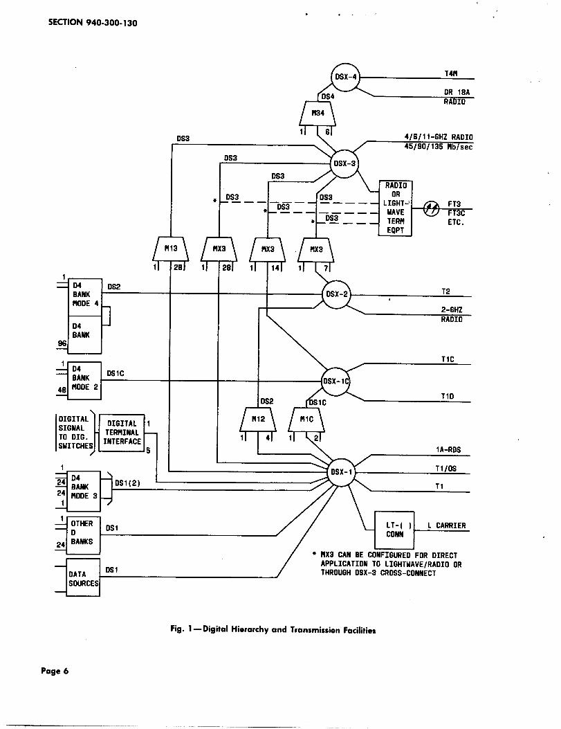
bandwidth and a minimum loading of 1152 voice grade circuits (VGC) in a 30-MHz channel. The latter require-ment coupled with economic factors has led to the development of several 6-GHz systems in the 78-to 135-Mb/srange capable of interfacing with one or more of the hierarchical rates DS1 at 1.544 Mb/s, DS2 at 6.312 Mb/s,and DS3 at 44.736 Mb/s. Figure 1 illustrates the digital hierarchy and locates 6-GHz radio among the transmis-sion facilities. The 6-GHz modulation techniques are typically 8-phase PSK or 16 QAM (quadrature amplitudemodulation). While available 6-GHz designs at the time of writing were single polarization per frequency trans-mission (SPF), dual polarization per frequency (DPF) systems employing 4-phase PSK are also accommodatedby FCC requirements. The following topics provide the transmission engineer with a review of certain FCC regu-lations that may influence selection and use of 6-GHz digital radio systems. This information, however, is notintended to replace AT&T Western Electric Practices or engineering letters (ELs) written to provide specificguidance, and questions should be directed to the appropriate headquarters FCC coordinator. The rules regard-ing digital radio systems fall within two basic categories

(a) Those which specify necessary equipment parameters and characteristics for type acceptance (manufac-turer)

(b) Those which specify distance and loading criteria for common carriers using the 6-GHz band (licensees).

The following topics first cover equipment parameters and characteristics which will have been specified bythe manufacturer prior to receiving FCC type acceptance. (Transmitters must be type accepted in accordancewith the FCC Rules, Part 21.) Distance and loading rules are then presented, followed by the stated requirementfor annual modulation and frequency checks. A discussion of additional guidelines then concludes the topics ofthis part.

B. Equipment Characteristicsand Requirements

2.o2 Following are the FCC definitions for bit rate, symbol rate, and modulation:

Bit Rate The rate of transmission of information in binary (2-state) form in bits perunit time.

Symbol Rate: Modulation rate in bauds. The term “baud” is derived from telegraphy anddescribes the symbol or information pulse rate. For example, if the fourpermutations available in two bits 00, 10, 01, and 11 are each represented asone of four carrier phase states 0°, + 90°, -90°, and 180°, each baud will, inthis case, represent two bits.

Digital Modulation: The process by which some characteristic (frequency, phase, amplitude, orcombinations thereof) of a carrier frequency is varied in accordance with adigital signal; e.g., one consisting of coded pulses or states.

SECTION 940-300-130● . .,,

T4M

OR 18ARADIO

P134

11DS3 4/6fll-13HzRADIO

45/90/135 t4b/sec

DS3

AM131 281

ITD4 0s2BANKMODE 4

D4BANK

96

A● DS3—

flx3

1 28

DS3

(& “ “

RADIO

DS3 OR.— ——— _

● 0s3 LIGHT-’ FT3——— ___ _

, DS3UAVE FT3C

——— TERM ETC.EQPT

MX3 RX3

1 141 1 7

I T2,

I2-GHZRAOIO

TIC

DS2TID

Mlc

11 I 41 11 <21

\DIGITALSIGNAL

DIGITAL 1

TO DIG.TERMINAL

SWITCHES INTERFACE.5 I lA-RDS

1 T1/OS7J-JD4— BANK ‘DS1(2)

24 MODE 3T1

1

J- OTHER[ 1

— 0DS1

24 BANKS

DATA 0s1

SOURCES

wPlX3CAN 6E CONFIGURED FOR DIRECTAPPLICATION TO LIGHTUAVE/RADIO ORTHROUGH DSX-3 CROSS-CONNECT

Fig. l—Digital Hierarchy and TransmissionFacilities

r

1SS2, SECTION 940-300-130

Emissionlimitation

2.03 Emission limitations for analog and digital radio equipment are different. For 6-GHz digital radio equip-ment, the modulated transmitter emission limitations are: the mean power emitted in any 4-kHz band

outside the authorized bandwidth shall be attenuated below the mean power in any 4-kHz band within the au-thorized bandwidth in accordance with the following formula. The attenuation should not be less than 50 dB,although attenuation greater than 80 dB is not req~red. (See Fig. 2.)

A = 35 + 0.8(P-50) + 10 log10 1?

where:

A = Attenuation (in dB) below the mean output level

P = Percent of authorized bandwidth removed from the carrier frequency,,

B = Authorized bandwidth in MHz.

mm‘oW-a=30<Wul-suaZs&1-e

.. . . -

~ IN CHANNEL~

100 I 1 I I 1 1 I 1 I 1 I I 1 I

-30 -15 0 +15 +30

FREQUENCY (MHz ) RELATIVE TO ASSIGNEO FREQUENCY

Fig. 2—FCC Emissionlimitation Mask

SECTION940-300-130

Necessary kndwidth Calculations

2.04 Formulas for calculating the necessary bandwidth (Bn) for digital modulation are contained in Part 2of the FCC Rules. The symbol “Y” at the end of the emission designator, 30000F9Y, indicates digital mod-

ulation.

Occupied 8andwidth

2.05 The occupied bandwidth shall be measured at the output of any filter network, pseudorandom generator,or other device required in normal service. Additionally, the occupied bandwidth shall be shown for any

spectrum-modifying device that is operated at the equipment user’s option.

Required TransmitterCapacity (Dtgital Traffic)

2.06 The minimum transmitter bit rate, in bits per second, shall be equal to or greater than the bandwidthspecified by the emission designator in hertz; i.e., to be acceptable, equipment must transmit one or more

bits per second per hertz.

Required TransmitterCapacity (VoiceTraffic)

2.07 Equipment to be used for voice transmission shall be capable of satisfactory operation within the autho-rized bandwidth when loaded with at least 1152 voice channels.

C. Distanceand Loading Rules

2.08 The following topics highlight those items which must be taken under consideration by the users (operat-ing companies) of 6-GHz digital radio systems.

Maximum Authorized 8crndwidth

2.09 The maximum authorized bandwidth for the 6-GHz common carrier band is 30 MHz.

Path Length

2.10 For the 6-GHz band, the minimum path distance is 17 kilometers (10.6 miles). However, the FCC maywaive this requirement if a showing (with supporting facts) can be made justifying a shorter path length.

Loading

2.11 In the 6-GHz band, the initial working channel must have an anticipated loading (within 5 years or otherperiod subject to reasonable projection) of at least the following

Voice Channels (4 kHz)–900

or

Digital Data–10 Mb/s

Frequency-diversity channels will be authorized only if the anticipated system growth will reach three workingchannels within 3 years.

II1SS 2, SECTION 940-300-130

D. Checkof Modulation and FrequencyCharacteristics

2.12 The modulation characteristics of digital radio equipment must be measured annually. The manufactur-er’s equipment-type acceptance filing contains the parameter(s) which, if measured and found to be in

tolerance, will ensure that the modulation characteristic remains within limits. The user should determine theseparameters from the manufacturer and measure them during the annual check. Frequency sources which canaffect the transmitted carrier must also be periodically checked, with intervals dependent on stability. Bothmodulation and frequency checks are further discussed in conjunction with maintenance considerations in Part3.

E. Additional Guidelines

FrequencyPlan

2.13 It is recommended that 6-GHz digital radios be operated on the regular 6-GHz T channels; i.e., 29.65-MHzchannel spacing with 5945.2 MHz the center frequency of the lowest channel (Fig. 3). Other frequency

plans have been used for analog radio systems in this band; e.g., splitting the frequency assignment of a channelto obtain two frequency assignments for short-haul radio systems. At this time, the only available systemsmeeting the FCC requirements outlined in Part 2A, B, and C above require a full 30-MHz channel. The 6-GHzband can be used best with the regular 6-GHz T channels, both for all-digital and combined analog and digitalroutes.

Single VersusDual Antennas

2.14 Long-haul radio systems are operated with separate antennas for transmitting and receiving on eachpath. Short-haul radio systems have generally used only one antenna on each path for both transmitting

and receiving. With single antenna systems, there is a risk that the higher power transmitters used in recentshort-haul systems may produce intolerable modulation products in the waveguide system. Thus one-antennaoperation cannot be used on systems where more than four of the available eight channels will be required. Anexpanded discussion of the intermodulation problem can be found in Section 940-384-100 (11 GHz).

Irrtermodulation

2.15 Figure 4 shows the potential 2A-B products. (The figure shows channels 21 through 28 transmitting andchannels 11 through 18 receiving. Adj scent repeater stations interchange transmitters and receivers.)

The diagram at the upper left is a portion of the frequency plan with the channel center frequencies identifiedby counting up from the lowest frequency channel. This notation is used in the rest of the figure to calculatethe location of the 2A-B modulation products. The midpoint of the 2A-B product spectrum is located at 8.5–(nz—2111) channels above f&In the example, this quantity is equal to 2.5. This is one-half the channel spacingabove the center of CH12. The 2A-B spectrum extends for 1.5 channel spacings at each side of its center, or fromthe center of CH1l to the center of CH14, i.e., 2.5 + 1.5 = 4 and 1. The broad digital spectrum extending almostto the edge of its assigned channel accounts for the wide spread.* Figure 4 shows that 2A-B products are avoidedby using any four consecutively numbered channels; e.g., transmit CH 22,23,24,25 or CH 12, 13,14,15, or CH25 through 28 or 15 through 18. The choice of CH 21 through 24/11 through 14 followed by CH 25 through 28/15through 18 on the second antenna provides for easy growth to full route capacity. Beginning with 25 through28 offers the same advantage.

*Not shown in the figure is the equation for transmitters in the lower band.

Product center = f.+ 8.5Af + [(2n2–nl)– 8.5]Jf

The bracketed coefficient of Af identifies the receiving channel number in the upper band.

1

SECTION 940-300-130

2-6

POLARIZATION

6404.8

6375.2

6345.5

6315.9

6288.2

6256.5

6226.9

6197.2

6152.8

6123.1

6093.5

6083.8

6034.2

6004.5

5974.8

5945.2

H vOR

H v

v H v H

--El I> 16Ill

I+-----m> i

12

+-----mI 12

I <

m----+Fig. 3—Frequency Plan

2.16 Using the five highest channels and the five lowest channels will permit up to five channels on one an-tenna without 2A-B product exposure.

Analog and Digital Systemson the Same Route

2.17 The spectrum of a digital radio system is relatively uniform across the channel, resulting in a typicalenergy spread (spillover) beyond the channel edge which is higher than that of FM signals of comparable

capacity. This results in more adjacent channel interference into analog channels. The spectrum of a digitalchannel is a function of the modulation or baud rate and, as discussed in Part 8 (interference), the availablecross-polarization discrimination (XPD) will not always be sufficient (at 30-MHz channel separation) to provide

(

I

,

1SS2, SECTION 940-300-130

(~’f”+’’f’+~bf* *x ● ●

* ●

CH 22~–: (fo+8.5Af)+~f

A’

CH 21 (fO+8.5Af)+~Af

——— ——— .l.~A~ — —

r

JEF~+~f----● ●

R*

● ●

%&fO+2Af

[&fo:Af

——— — — ‘O=CH 11-A’

=5915.5 HHz

2A-B PROOUCTS

A=(ffJ+8.5Af)+nlAf

8=(fO+8.5Af)+n2Af

UHERE n2>nl

fo=cH 11-Af=5’1505 MHz

Af%29m6~z

THEREFORE

2A-B=(fo+8.5Af)-(n2-2nl)Af

EXAHPLE: nl=l(CH 21)

n2s8(cH 28)

PROOUCT CENTER AT:fo+’.5Af-(’-2)Af

❑ ‘0+2.5A’ = 59”.5 HHz

MIOUAY CH 12 ANO CH 13

SPECTRUM SPREAO

FROM: fO+l.OAf(~ 11)

TO: ‘0+4.OA’(CH 14)

TUOUORKA8LE PLANS

FOR SINGLE ANTENNA OPERATION (NOTE 1)

USE CH 1-4

XMT CH 21-24 REC CH 11-14

2A-B UITHnl=l(CH 21)n2=4(CH 24)

2A-B=fo+8.5Af-(4-2)hF

=fo+e.mf

SPREAO: ‘o+&f m lB

fo+~f CH 15

USE CH 5-B

X14T CH 25-28 REC CH 15-18

2A-8 UITHnl=5(CH 25)n2=8(CH 28)

2A-B=fO+8.5Af-(8-10)/iF

=f(j+lo.af

SPREAD : fO+9A f

1(ALL IN XMTG BANO)ffJ+12Af

(NOTE 1)ANY OTHER 4 CONSECUTIVE CHANNELS ARE ALSO POSSIBLE, I.E., CH2-5,CH 3-6, CH 4-7. IF A SECOND ANTENNA ANO FULL SYSTEM GROWTH ISOESIREO, THE PLANS SHOUN PERMIT GROklTH WITHOUT REARRANGEMENTS.

Pig. 4-2A-B Products (6 GHz)

!,

SECTION940-300-130

the required discrimination. In such cases, an unoccupied channel must be interposed between otherwise adja-cent digital and analog channels operating on the same route.

2.18 The transmitted spectrum of the digital radio must permit operation, on the same hop, of an analog FMradio channel with a center frequency separation of 59.3 MHz and like polarization. The digital radio

spectral requirement that must be met for a transmitter with a nominal output power of P dBm is stated inparagraph 2.19.

2.19 The power density in a 4-kHz band at a frequency of (50.776–S) MHz from the center of the digital radiochannel shall be at least (75+P) dB below the measured transmitter power in dBm. S is the sum of the

maximum frequency tolerances (in MHz) of the two transmitters. This requirement will limit the adj scentchannel interference noise into the highest frequency baseband circuit of the analog radio to 4 dBrncO or less.That circuit is nominally located 50.776 MHz from the center of the digital channel.

2.2o The digital radio should permit operation of an analog FM radio with a center frequency separation of44.5 MHz (split frequency plan) or 29.65 MHz. In this case, the frequency cited in paragraph 2.19 would

be decreased by 14.8 MHz or 29.65 MHz, respectively. The attenuation limit(s) would be unchanged. For adjacentchannel separation, a nominal 30 dB of cross-polarization isolation is to be assumed.

3. SYSTEMCHARACTERISTICSAND OVERVIEW

A. General

3.01

(a)

(b)

(c)

(d)

(e)

(f)

(g)

This part discusses items and characteristics of particular significance to digital systems. Topics include:

Fade margin

Interference

Bit error rate

Modulation types

Repeater types

Alarming and maintenance

Upfades.

A knowledge of the system fade margin is needed to calculate and predict outage. The theoretical fade marginbased on thermal noise criteria will be combined with the deleterious impact of multipath phenomena and inter-ference (rain fading is insignificant at 6 GHz) to arrive at practical values for estimating system outage. Theinitial determination of the fade margin considers system gain and section loss and is supported by Fig. 5.

B. TheoreticalFade Margin

3.02 The theoretical fade margin (F) is found from the relationship SG = SL + F where:

SG = System Gain

SL = Section Loss

F = Fade Margin.

,,, !,

1SS2, SECTION940-300-130

II1r~

I 4’;>L 4!T

II

r–+ ————1

~–L––––--J

A

!r– -–––7

I I I

‘–T––––JII

II

SECTION940-300-130

System gain is determined by equipment design characteristics and is therefore controlled by the manufacturer,while section loss is controlled by the route designer.

System Goin (SG)

3.03 System gain gives the thermal noise performance measure of the radio equipment alone. System gainis defined as the difference between the nominal power (in dBm) measured at the transmitter bay output

(see location on Fig. 5) and the minimum power (in dBm) at the receiver bay input for acceptable radio systemperformance. (Note that the stipulation of acceptable performance includes the receiver as necessary to thisevaluation— a point which might be overlooked with strict reference to the specified measurement locations inFig. 5.) Typical acceptable performance is defined as minimum receiver input power such that the following cri-teria are met

Analog Systems: Maximum noise level (worst message channel) = 551dBrncO

Digital Systems Maximum bit error rate (BER) = 10-3.

3.04 It should be recognized that this definition of system gain gives a performance measure of the radioequipment alone. System gain will go up with such factors as higher transmitter power and lower re-

ceiver noise figure. System gain does not depend on antenna sizes, waveguide, or path lengths, nor does it includethe effect of any interferences. For a higher system fade margin (F), the section loss must be reduced to main-tain the minimum power at the receiver. This minimum power for acceptable performance depends on the inter-nal thermal noise and the losses within the radio bay, i.e., filters and other networks. It should also be notedfrom Fig. 5 that the system gain (SG), as defined by (SG = SL + F), will be smaller than the quantity [P.O~,,an,–P * ~in] (the difference of transmitter power and minimum received signal as measured at the respective bayoutput and input) by the amount of the channel combining and separating filter insertion losses. Formultichannel systems, the losses of several tandem filters are incurred. A high value of system gain alone doesnot guarantee good performance.

SectionLoss(S1)

3.o5 Section loss is defined as the total power loss between a transmitter bay output and the succeeding re-ceiver bay input during normal propagation conditions. It is completely controlled by the route design

independent of the chosen radio equipment. It is the sum of the losses over one hop due to all station and outdoorwaveguide runs and network losses plus the nominal free space path loss minus the gains of the antennas. Anexpression for SL can be written in terms of these component losses as

SL = L~S + LW~~(j~+L - G,, - G~AN‘TOT

where

LM = Free-space path loss

LW,;~,)~= Total waveguide losses (transmitting and receiving)

LN\i’T(,T= Total network losses (transmitting and receiving)

GTA = Gain of transmitting antenna

GRA = Gain of receiving antenna.

1SS 2, SECTION 940-300-130

A distinction should be made between microwave facilities which handle only 6-GHz radio traffic and thosewhich handle a mixture of 11-, 6-, and 4-GHz traffic over shared waveguide and antenna components. Theselatter systems are termed “combined systems” and incorporate additional microwave networks whose lossesmust be included in L~ Additional specifics related to network, waveguide, and antenna combinations andchoices are provided in Part 9.

Wa veguide Loss

3.o6 All waveguide in the path from a transmitter bay up to the antenna port and from the receiving antennato the receiver bay input must be included in the calculation. Waveguide losses range from 2 dB to about

10 dB depending on length, size of the guide, and its geometry–rectangular, elliptical, or circular. The choicesare closely coupled with the choice of antennas.

Net work Losses

3.07 A dual-polarized 6-GHz-only radio system which uses a single vertical waveguide run requires polariza-tion combining networks and, if transitions to other waveguide geometries or sizes occur, transition net-

works and mode suppressors. In combined systems (4/6/11 GHz) using a common vertical antenna feed-run andantenna, combining networks are required to couple the frequency bands into the waveguide. In some cases,mode suppressor networks may also be required. Each such network contributes to the total section loss throughreflection and ohmic losses. Since these networks are usually short, the ohmic loss contributions are very small,and with correct design, reflection losses can also be minimized. Typically, each such network will introduce0.2- or 0.3-dB loss.

Free-Space Path Loss

3.08 The geometric spreading of energy radiated from the transmitter location to the receiver locations re-sults in the free-space path loss, LFs (see Section 940-310-101 for detailed discussion). This contribution

to the overall section loss (in dB) at the midband frequency of 6.2 GHz is given by

L~, = 112.5 + 20 log D (miles)

= 108.3 + 20 log D (kilometers)

where.

D is the path length in miles or kilometers.

Thermal Noise Fade Margin (F)

3.09 The theoretical or thermal noise fade margin (F) of a hop is the difference between the system gain andthe section loss as discussed above, and is expressed as

F= SG– SL.

C. Fade Margin ReductionsCaused by Interferenceand DispersiveFading

3.10 For many analog systems of the past, F was the margin that was available to cover propagation distur-bances (fades). Higher system gains or lower section losses would lead directly to better performance.

One limitation that has always been present is interference (both from within a system and from externalsources). Since the definition of system gain excluded all interference effects, F is the thermal noise margin forflat fading in the absence of interference.

SECTION 940-300-130

3.11 For 6-GHz digital radio systems, an even greater fade margin limitation is imposed by distortion (disper-sion) resulting from multipath fading. Dispersion can occur even during relatively shallow fades. Distor-

tion introduced by multipath can cause high bit error rates (BER) well before fade levels reach the thermal noisemargin. When either interference or multipath distortion effects are controlling, the well-known means to in-crease F—such as added transmitter power, larger antennas, or lower noise figures and waveguide losses—are not very effective in reducing outages.

3.12 For these reasons, the unqualified term “fade margin” will seldom be used. Instead, the more specificterm “thermal noise margin” (F) and a new term “dispersive fade level” for use in calculating multipath

outages will be employed. Dispersive fade level relates the total outage time (high BER periods) observed indigital system experiments to the single frequency multipath fading time observed on the same path. The fadedepth for which the measured time below level is the same as the observed high BER time is taken as the disper-sive fade level. Part 6 provides methods for combining the thermal noise margin and the effects of interferenceand dispersion to obtain a composite fade margin.

D. Interference

Cochannel

3.13 In digital transmission, the transmitted power is uniformly distributed across much of the radio channel;there is no strong carrier, such as in low index FM. The interference conditions over a narrow bandwidth

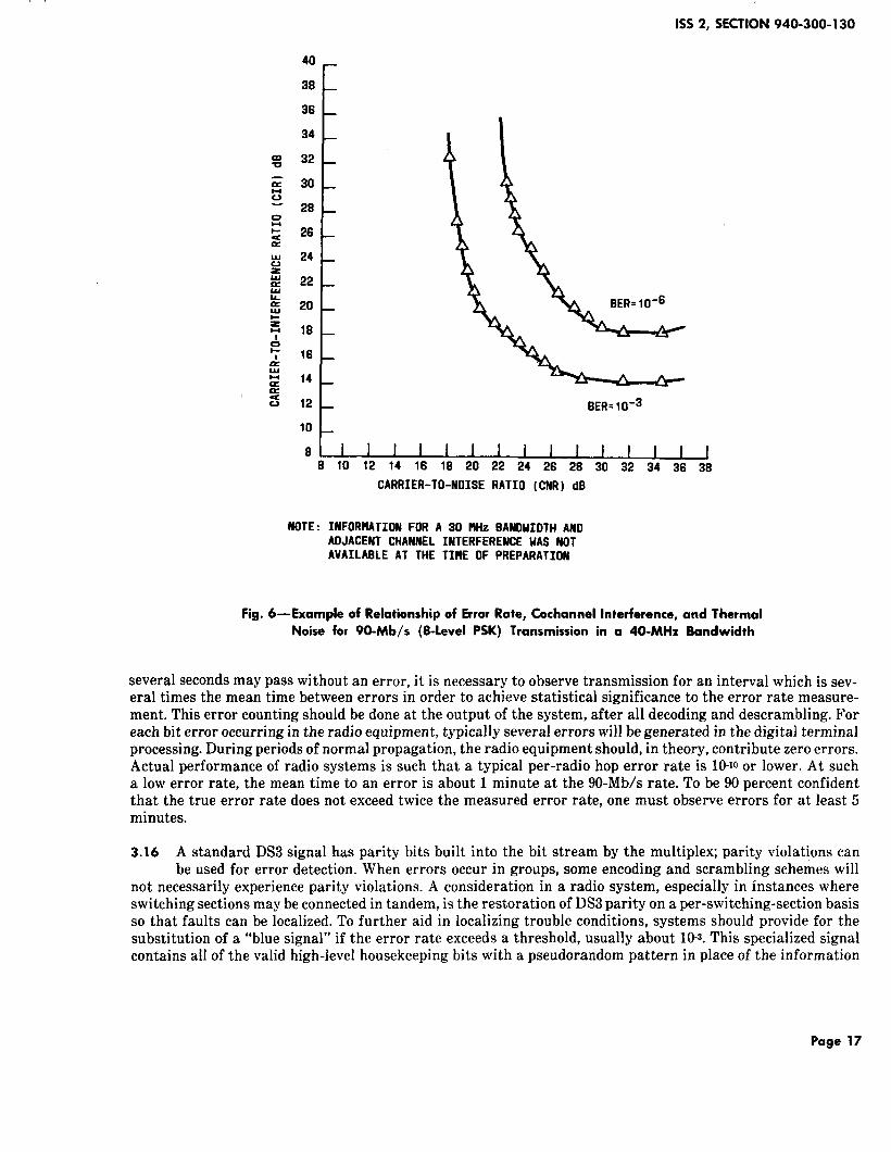
(such as 4 kHz) do not affect a particular VF circuit carried by the digital signal. The interference tolerancein digital transmission depends upon the total interference power accepted by the receiver; the interference af-fects all voice circuits in the digital signal equally. The tolerance to interference can be characterized by its im-pact on the system gain: a C/I of X dB will degrade the system gain by 1 dB. The C/I for cochannel interferenceresulting in a l-dB degradation will range from a theoretical minimum of 24 dB to perhaps as high as 30 dBin practical systems. Figure 6 presents an example, based on measured data, of the relationship of BER, C/I,and C/N (thermal noise). Note that the channel bandwidth in this example is 40 rather than 30 MHz (the onlydata available at the time of writing) and therefore is included for illustrative purposes only.

Adiacent Channel

3.14 With high-capacity digital transmission, some signal energy will necessarily spill over into the adjacentchannel even when the transmitted spectrum satisfies the FCC Rules on emission limitations. Further,

due to necessary compromises in the receiver filtering, there will be receiver sensitivity to signals in the adja-cent channel. Thus adjacent channels have a degrading effect on the system gain of a digital radio. At 6 GHz,the frequency plan calls for adj scent channels to be on orthogonal polarizations. This aids in the discriminationbetween adjacent channels. A typical statement of a radio system’s sensitivity to adjacent channel interferencemight be: a C/I of Y dB for each of the two adjacent channel interferences will degrade the system gain by1 dB. This will provide an indication of the value of cross-polarization discrimination that must be maintained(including fading periods) for a tolerably small influence of the fade margin. The amount of adjacent channeldiscrimination achieved by transmitter and receiver filtering is a function of adjacent channel spacing. The nor-mal channel spacing, center to center, is 29.65 MHz for the frequency plan. To fully develop a route, the radiosystem should be designed to operate at this channel spacing. The topic of digital-into-analog interference isdiscussed in Part 8.

E. Bit ErrorRate (BER)

3.15 Bit error rate (BER) is the fraction of bits received incorrectly relative to the total number transmitted.Usually this quantity is measured under some steady state condition so that the bit error rate is the ratio

of the number of errors per second to the bit rate in bits per second. The BER may be measured at the DS3 rate(44 Mb/s), the DS1 rate (1.5 Mb/s), or at any multiple or submultiple of these rates. Since at low bit error rates

1SS2, SECTION940-300-130

40 ~

38

36

34

32

30

28

26

24

22

20

16

16

14

12

L

8ER=1O-3

10

8 I I 1 1 I I 1 I I I I I I I I6 10 12 14 16 18 20 22 24 26 26 30 32 34 36 38

NOTE :

CARRIER-TO-NOISE RATIO (CNR) dB

INFORMATION FOR A 30 MttZ BANOWIDTH ANDADJACENT CHANNEL INTERFERENCE HAS NOTAVAILABLE AT THE TIME OF PREPARATION

Fig. 6-Example of Relationshipof ErrorRate, Cochannel Interference,and ThermalNoise for 90-Mb/s (8-Level PSK) Transmission in a 40-MHz Bandwidth

several seconds may pass without anerror, itis necessary to observe transmission for an interval which issev-eral times the meantime between errors in order to achieve statistical significanceto the error rate measure-merit. This error counting should bedone atthe output ofthe system, after all decoding anddescrambling. Foreach biterroroccurring in the radioequipment, typically several errors will degenerated in thedigital terminalprocessing.During periodsofnormal propagation, the radioequipment should,intheory, contributezero errors.Actual performance of radio systems is such that atypical per-radio hop error rate is lo-lo or lower. At suchalowerror rate, the meantime to an error isaboutl minuteatthe90-Mb/srate. To be 90 percent confidentthat the true error rate does not exceed twice the measured error rate, one must observe errors for atleast5minutes.

3.16 Astandard DS3signal hasparity bits built into the bit stream by the multiplex; parity violations canbe used for error detection. When errors occur in groups, some encoding and scrambling schemes will

not necessarily experience parity violations. A consideration in a radio system, especially in instances whereswitching sections may be connected in tandem, is the restoration of DS3 parity on a per-switching-section basisso that faults can be localized. To further aid in localizing trouble conditions, systems should provide for thesubstitution of a “blue signal” if the error rate exceeds a threshold, usually about 10-s. This specialized signalcontains all of the valid high-level housekeeping bits with a pseudorandom pattern in place of the information

SECTION940-300-130

bits. The blue signal keeps any following high-level multiplex or transmission equipment from alarming, or ini-tiating’protection switching, and thus aids in the fault location process, since only the section failed is alarmed.The blue signal can be considered analogous to the carrier resupply function in conventional analog radio.

3.17 During fading periods, degraded error rate performance may occur. Error rates better than 10-6are oflittle consequence in the digital transmission of voice since the noise is controlled by the PCM channel

banks. At a line error rate greater than about 10-s, voice transmission becomes degraded and the receiving PCMchannel banks cannot reliably stay in synchronization. Repeated misframe conditions degrade transmissionuntil the carrier group alarms (CGA) at the receiving channel banks operate, taking the banks out of serviceand disconnecting all calls in progress. At an error rate of 10-s,one can consider the transmission to be unaccept-able and, if the duration exceeds the CGA operation time, an outage results. [The CGA operates when the out-of-frame time exceeds a value specified for a particular channel bank: 300 milliseconds for D1 (except DID), D2,and early D3, and approximately 2 seconds for DID, later D3, and D4 channel banks as well as most digitalswitch terminations.]

3.18 Since an error rate of 10-6is unusual for properly functioning equipment, it is appropriate to request aprotection switch at, an average error rate of around 10-6.Some hysteresis should be built into the protec-

tion switching system so that an excessive number of switching events will not occur. Comparison of switchingactivity of the radio channels in the system is desirable. A departure of one channel from the average can bean indication of performance deterioration in that channel. From this discussion, one can see the importanceof two error rate values 10-6corresponding to a switch request and 10-scorresponding to an outage. System gainscorresponding to these error rates are of interest to the system engineer.

F. Modulation Types

3.19 At the time of writing, most 6-GHz digital systems meeting the FCC 1152-voice-circuit-per-channel re-quirement are 8 PSK (8-phase, phase shift keyed) with coherent detection or 16 QAM (quadrature ampli-

tude modulation–16 states). Both techniques permit capacities as high as two DS3S (approximately 90 Mb/s)to be achieved in a 6-GHz, 30-MHz channel. The linearity requirements to transmit the 16-QAM signal are moresevere than those of a typical 8-phase system, due to the multiple amplitude levels. However, the low baud rateof 22.63 Mbaud for the 90.524-Mb/s capacity reduces adjacent channel interference problems (see Table J) whentransmitting in a 30-MHz channel. Both the low baud rate and linearity requirements yield a transmitter spec-trum which is narrower than achievable from a 30-Mbaud system. The reduced adjacent channel interferenceeases full route (eight RF channels) operation with adjacent digital and analog channels.

G. RepeaterTypes

3.20 One of the most significant characteristics of a digital signal is the ability to reshape and retime, as wellas retransmit, the signal at each repeater. As previously noted, such regeneration offsets the cumulative

effects of distortion, noise, and interference. When a repeater amplifies and retransmits the received signalwithout reshaping and retiming, it is said to be a nonregenerative repeater. Since circuitry is eliminated by notregenerating, a cost reduction is effected. For example, if the interconnection is made at IF, then carrier recov-ery, timing recovery, demodulator, regenerator, and modulator circuits are not needed. However, the distortionsand interferences of each span add to one another, lessening the margin for error with each nonregenerativerepetition. Some of the disadvantages of a nonregenerative repeater are the lack of access to the baseband signalfor maintenance purposes, the possible loss of some fault location capability, possible difficulties associatedwith auxiliary channel transmission, and the cumulative effects of interference and distortion.

H. Auxiliary Channels

3.21 Auxiliary channel signals can be carried by digital radio either by multiplexing them into the main bitstream or by separate low-level amplitude or phase modulation. Separate modulation techniques always

cause some degradation to the payload, but they are relatively simple to implement. The modulation can providedigital or analog channels. Multiplexing additional bits into the payload bit stream slightly increases the bit

I

4 ,,

1SS 2, SECTION 940-300-130

rate to be transmitted and requires multiplexing equipment at each location where auxiliary channel access isrequired. On the other hand, this scheme incurs little, if any, degradation to the payload.

1. Maintenance Considerations

General

3.22 The following discussion is intended to enhance awareness of the hardware features and maintenanceprocedures needed for efficient operation of digital radio systems. In addition to maintenance informa-

tion of a fairly general nature (for example, FCC-required measurements), the relative merits of various typesof maintenance-oriented hardware will also be discussed. Familiarity with the capabilities and limitations ofthese maintenance aids will help in assessing the suitability of radio and test equipment for a particular applica-tion. The importance of maintenance considerations for digital radio systems should not be underestimated.Digital systems are inherently more sensitive to hard-to-find transient problems than analog systems, andmaintenance can become a nearly insurmountable task, even on relatively small systems, if the means providedfor detecting and troubleshooting problems are not thorough and efficient.

3.23 Early experience with high-speed digital radio has shown some marked contrasts with analog radiowhich will affect monitoring and maintenance practices and which could have a bearing on various per-

formance indices. Unlike analog radio transmission practices where noise and noise loading measurements aremade infrequently, and occasional bursts of noise are usually ignored, digital transmission may be monitoredcontinuously by means of parity bits and/or test patterns embedded directly in the bit stream. Test equipmentis becoming available to generate and monitor these test patterns at hierarchical access points within the digitalnetwork and to aid in locating defective units of the system. Continuous monitoring can be used to considerableadvantage from the early stages of installation onward to check for compatibility of subsystems such as multi-plexer, cross-connect fields, and protection switching systems.

3.24 The error performance as monitored should be characterized by long error-free periods, occasional iso-lated errors caused by marginal transmission on one or more radio hops during fading, short bursts of

many errors during multiplex reframing as a result of transients, switching operations, intermittent contactsor other short interruptions, and total outages which may be due to any cause. The need for engineering atten-tion to the causes of the various error conditions cannot be overemphasized. Maintenance activity as herein dis-cussed falls into three categories

(a)

(b)

(c)

FCC-required measurements and adjustments

Other routine maintenance activities aimed at optimizing adjustments and detecting “silent failures”before they become service-affecting

Fault location and general troubleshooting.

FCC Compliance

3.25 FCC compliance is relatively straightforward, as manufacturers are required to specify all periodic mea-surements needed to ensure that radio transmitters continue to operate within the rules. At specified

intervals, tests must be performed and results recorded in the station log. These tests and all other transmittermaintenance work which may affect the emitted signal must be done by, or under the immediate supervisionof, a person holding a general radio telephone operator’s license. The measurements (and possible adjustments)specified for meeting FCC requirements encompass two categories of tests

(a) Determination that frequency sources which may affect the transmitted carrier frequency are withinproper limits

, ,

SECTION 940-300-130

(b) Checks on modulation characteristics related to keeping the radiated signal within the proper limits.

3.26 The oscillator frequency test must be made annually if the oscillator units are crystal-controlled or regu-lated by temperature-controlled or temperature-compensated cavities. If they are not so regulated, oscil-

lator frequencies must be checked monthly. Modulation characteristics must be checked annually. The bit ratecan usually be checked by measuring the frequency of an associated clock signal in the transmitting digital ter-minal. Unlike the tests for verifying the correct carrier frequency which must be done for every hop, the testto determine the bit rate need be done only at the first transmitting digital terminal. All other bit-rate clockson the same channel will be locked to this one, and should any one of them malfunction, the system will failimmediately. (Blue signal generators are an exception, in that each must be checked separately.) Routine trans-mitter power measurements, although not required by the FCC, may be done as often as specified by the manu-facturer. Power measurements must, of course, be done at every hop.

3.27 Since fulfilling FCC maintenance requirements consists of performing a limited number of very specifictests, and since failure of any test is almost always remedied by readjustment or direct replacement of

the unit under test, there is no anticipated difficulty in meeting FCC obligations. Careful planning can signifi-cantly reduce the difficulties encountered in making measurements and adjustments of critical circuits. Mostmeasurements and adjustments required by the FCC can be done “in-service.”

Other Routine Maintenance

General

3.28 While fairly definite statements could be made about the type of measurements required by the FCCRules, there is much less certainty about other routine maintenance. Differences in equipment design,

and even differences in maintenance philosophy, can lead to wide variations in the type and amount of routinemaintenance recommended. Nonetheless, some general remarks can be made to help the user assess the recom-mended maintenance program. The user is responsible for taking adequate safeguards to prevent loss of service.

Routine Adjustments

3.29 There are usually very few adjustments on modern radio systems which need to be made on a routinebasis (excluding FCC-required adjustments). Those which remain usually represent a compromise in

favor of manual maintenance in place of increased system cost and electronic complexity, or they provide a fine-grained adjustment of some parameter which adds enough margin to warrant access. The types of routine ad-justments which might be recommended could include setting a critical power supply voltage, adjusting thephase of a signal, “tuning-up” a power amplifier, etc. As a guide, one or perhaps two routine adjustments perone-way radio channel per hop would not be excessive. Much more than this could mean excessive maintenancecosts which could easily offset any initial savings over buying a system equipped to take care of such thingsautomatically. It may be possible or desirable to simply abstain from all routine adjustments (except those re-quired by FCC Rules) in favor of demand maintenance. This reduces costs and lowers opportunities for operatorerrors which statistically are bound to occur. However, there is a trade-off to be dealt with which will be dis-cussed below.

Routine Tests to Detect Silent Failures

3.3o A second form of routine maintenance is the discovery and repair of “silent failures,” i.e., those due tocomponents or subsystems which when they fail do not immediately affect the performance of the radio

equipment. Instead, these failures simply exist with no observable consequences until some new set of circum-stances makes them obvious. As a partial list of examples, consider the consequences of loss of AGC range inan amplifier, poor receiver noise figure, or loss of fade range due to erroneous slicing levels in a digital receiver.In unfaded conditions, none of these matter. When fading does occur, any of them can cause premature failureof the channel. Without some form of routine maintenance program to detect them, equipment problems may

—- —

,,

1SS2, SECTION 940-300-130

be diagnosed as statistically excessive fading. This same sort of undiscovered “loss-of-margin” difficulty canbe experienced as a result of demand (rather than routine) adjustment of critical system parameters.

3.31 The previous examples of silent failures were all of a kind such that, if fading did occur and the channeldid fail prematurely, the protection switching system would take over and prevent a loss of service. This

would remain true up to a point, but unbalanced or excessive demands on the protection channel would eventu-ally lead to an overall reduction in reliability. Another type of silent failure is one which eventually leads toloss of service. For example, the performance monitor which must initiate a protection switch may be quietlyfailed. The actual switch, the protection switch signaling, coding, and decoding apparatus are all similarly vul-nerable. (Failures of this type are further considered under equipment outage, Part 7.) These are all subsystemswhich may fail to do their jobs and may thus cause an unnecessary service failure if routine maintenance checksdo not assure that they are operational. In short, use of equipment which automatically exercises all off-linefunctions and all features which are not used or tested on a regular basis is recommended.

Fault Sectionalization and Localization

General

3.32 The most difficult aspect of maintenance is troubleshooting. In this respect, digital systems are harderto maintain because they are more complex than analog systems; i.e., while radio equipment can be simi-

lar, terminal equipment is more complicated. Whereas an FM receiver contains tuned circuits, a rectifier, andlinear amplification, a digital terminal receiver may include multiple phase-locked loops, multipledemodulators, combinational logic circuitry, and numerous timing and framing signals and associated hard-ware. In most analog systems, repeater stations have only microwave radio equipment and no terminal equip-ment. Digital systems often employ regenerators at intermediate stations, making these stations nearly ascomplex electronically as terminal stations. In addition, the ability of digital systems to regenerate and elimi-nate cumulative distortions on multihop systems also means that simple analog test signals can no longer beroutinely sent from one end of a system to the other as a means of providing a quick, overall check of perfor-mance. An analog test signal would be blocked upon encountering the first regenerator. Finally, digital systems,despite their inherently rugged nature, are much more sensitive to transient problems than analog “systems.Submillisecond transient phenomena which were not considered significant to analog communications nowshow up as thousands of bit errors and sometimes as losses of frame throughout the digital hierarchy beingserved by the radio system. These problems can sometimes be ignored without penalty if the payload is entirelydigitally encoded voice, but if data is to be carried, such transient problems should be substantially eliminated.As a practical matter, the ability to determine that bit errors are occurring will mean that maintenance crewswill be called upon to eliminate them regardless of the nature of the payload. This may not be lost effort sincetransients often foretell more serious problems ahead, but it does present a significant maintenance challenge.

Troubleshooting and Protection Switching

3.33 Troubleshooting techniques are partially determined by the type of protection switching used. Hot-standby protection (with or without space diversity) restricts testing to equipment tests at individual

repeaters; out-of-service testing of a channel over tandem hops is not generally possible. Frequency diversityallows out-of-service testing on a switching section basis. Figure 7 is a block diagram showing the major compo-nents of a digital radio protection switching section for a single one-way channel. A switching section can beseveral hops long, and will probably have regenerators at most intermediate stations, although there is the pos-sibility that some radio systems will be configured in such a way that a straight-through connection from theradio receiver to the radio transmitter will be allowed at some intermediate stations. (Such stations would thenbe termed repeater stations rather than regenerator stations.) The digital terminal transmitter at the head endof the system processes the high-speed digital signal before it is transmitted over the radio, and the digital ter-minal receiver at the receiver end of the switching section takes the signal out of the format required for radio

SECTION940-300-130

transmission and puts it back into the format required for transmission to the receiving multiplex. Regenera-tors are normally composed of some fraction of the circuitry required for a digital terminal receiver and a digitalterminal transmitter.

3.34 Each end of the system is equipped with a radio protection switch. Signaling may be required betweenthe ends to coordinate switching actions. Some type of performance monitor at the receive end of the

system monitors the received signal and is responsible for initiating and releasing protection switches. Dropand add repeaters (Fig. 8) or junction or spur routes (Fig. 9) may be included within a switching section in somesystems. Overall economy may result from these arrangements even though more complex command and con-trol logic is needed than would be necessary with simple section switching.

Failure Sectionalization

3.35 One immediately apparent maintenance consideration concerns failure sectionalization between theradio system, the multiplex, and the channel banks. Some radio/multiplex systems may employ a system

of blue signals which can be automatically switched onto the line to prevent alarming of downstream equipmentdue to the failure. Alternatively, the alarm system maybe setup in such a way that multiplex and channel bankpersonnel have easy access to radio performance information. In this way, alarming in multiplex and channelbank units can be ignored when it is clear that the radio system is at fault.

In-Service Performance Monitoring Options

3.36 Performance monitoring is paramount to digital system maintenance. It is difficult, if not impossible,to troubleshoot a digital system efficiently if the performance monitor cannot detect varied types of fail-

ures in radio, regenerator, or digital terminal equipment. (This is especially true in systems consisting of multi-ple switching sections.) Not only is the job of troubleshooting made much more difficult in such a situation, butthe transmission availability of the system will be in serious question. The performance monitor is responsiblefor issuing protection switch requests. It cannot perform this function adequately if it cannot detect all typesof failures. Two general types of in-service performance monitors will be discussed. They are:

(a)

(b)

3.37

Those which rely primarily on “eye-opening” measurements, supplemented by numerous activity detec-tors and other alarms

Those which rely primarily on the measurement of parity violations, sometimes supplemented by activitydetectors and alarms.

So called “eye” diagrams are an oscilloscope fimme formed by superimposing all possible pulse sequencesover a dura_tion of-two signaling intervals. The measurement of eye-openi~g is basically a measure of

margin against error made on the analog signal delivered to the digital terminal receiver by the radio, and ismade after demodulation but before the signal is regenerated. Eye-opening measurements can detect failuresdue to intersymbol interference, excessive radio thermal noise, and interference along the radio path. Thus,most microwave radio problems can be detected in this way. However, eye-opening measurements are almosttotally ineffective against digital problems which may occur in regenerators and terminals. For this reason,they should be supplemented by activity or “energy” detectors which monitor various critical points in an effortto detect catastrophic failures which result in loss of signal within the digital terminal. A shortcoming to activ-ity detectors is that they leave undetected a significant class of failures those failures of combinational logiccircuitry and other subsystems which do not result in loss of activity. The outputs of logic gates and flip-flopsdo not necessarily freeze when marginal conditions exist or failures occur. Data can continue to flow, but it willcontain errors, many times to the extent that the system becomes totally unusable. Digital terminals and regen-erators can contain scramblers, coders, countdown circuits, and numerous other circuits which are digital innature and which may fail in this manner. For these reasons, the detection of parity violations is a powerfulmonitor of performance. Parity monitors examine the received signal after it has passed through all of the cir-cuitry mentioned above. The framing pattern of the signal is detected and the monitor locks into the parity bitwhich was inserted by the multiplex at the head end. By comparing the parity bits to groups of received data,

=ol-l1-Vu

-1xLu.A

51-

=h_#-

ao E

1-a u 1-UJ u H

u074 z 0?5WW Id HZ THROUGH OTHERcl~ @ n<

w u= REGENERATIONaa m a+ STATIONS

+ :- : “l”fl+l-@J*I REGENERATION STATION

I

ISIGNALING

1 1L ---- .-HEAO-END

CHANNELBANKS

—--- ——-- —- 1sz Auld‘= J<=>ii I-HI-4

H

II-lzlu

1- H+ C5uu no-1 OH

I-IIJJLUz

IUz n+= :%

ax acn

[

I

— I●

● - I● I

I II PERFORMANCE

I SWITCHMONITOR

I REQUESTU

L-Z RAoIO SWITCHINGSECTION

.Fig. 7—Radio Switching Section—BlockDiagram

.

SECTION 940-300-130

DRDP AND ADD REPEATER

-e

44.7

-e

-a

44.7

-e●

●

●

●

●

D

fluxXMT

44.7

l:N S1(XMT)

I r ——— ——

“=EI+-EI————

[

H1

I II II DSA I

I I 1 I

4“’C”I=I’’’M’’IIXMTI

‘–I–––––––I–J+ 4 CDMMAND PATHSI

I:nlSI(RCV)

PROT

T

b

44.7

b

>

44.7

>●

●

●

●

●

E

MUXRCV

44.7

Fig. 8— 1:N With Drop and Add Repeater (90-Mb SystemShown)

the performance monitor can detect digital errors regardless of their source. Obviously, to be totally effective,the performance monitor must examine the data stream at the very end of the system. For various reasons, thisis not possible. Some small amount of circuitry may follow the performance monitor, in which case activity de-tectors should be used on this circuitry to supplement the process of monitoring parity violations. Examinationand comparison of the time history of performance monitor records can point to radio channels that have sub-normal performance. Finally, it should be added that monitoring bipolar violations is generally an unsuitableway to determine the performance of the digital radio system. The digital signal is normally stripped of all bipo-lar characteristics early in the process of preparing the signal for radio transmission. The bipolar format is usu-ally reinstated at the very output of the radio digital terminal receiver. Thus, failures of the digital and/ormicrowave radio equipment have no connection to the bipolar format.

3.38

(a)

(b)

The sources of background errors on a multihop digital radio route are not easy to troubleshoot because: -

Most of available digital radios lack a per-hop indication of background errors

Most background errors do not affect message telephone service (MTS) and do not initiate remote alarmsor carrier group alarms

,, I

1SS2, SECTION 940-300-130

r44.7 ‘ZNXHT

44.7

44.7

: Dp : - : : ‘} : :

XMT z RCV XMT + RCV 44.7

1:1 1:1XMT

44.7 RCV

* + -9

PROT PROT PROTI

NOTE COMMANO PATH

1:1 XMT

COHHANOPATH

XMT XMTPROT

RCV RCV XMTXMT

PROT PROT4

77

1:1 RCVII

1:1 XHT

COMMANOPATH

NOTE:CONNECT TO OPPOSITEOIRECTION OF l:N ROUTE(NOT SHOWN)

44.7 44.7

Fig.9— l:N With Junction

SECTION940-300-130

(c) Some background errors initiate short intermittent local alarms. However, radio fading can also causeshort intermittent alarms. The fading-caused alarms are confusing to a craftperson attempting to locate

equipment problems.

3.39 The existing maintenance procedure requires tedious and time-consuming out-of-service tests to locatethe trouble source. Based upon these experiences, the following additional features are desirable for fu-

ture digital radio to carry the more demanding digital services such as PICTUREPHONE@ Meeting Service(PMS), DDS, etc.

(a)

(b)

(c)

(d)

Detection of background errored second on a per-hop basis using some coding schemes such as paritycheck and parity restoration on every hop

Separate fading-caused error seconds from equipment generated background error seconds (e.g., useAGC voltage for fading indication)

Count errored seconds per day per hop excluding fading-caused errors

If the number of errored seconds per hop exceeds the objective in a 24-hour period, initiate local and re-mote alarms so that the alarm center can immediately dispatch a craftperson to the trouble station for

correction.

Alarming and In-Service Fault Locating

3.4o Regardless of the method used for performance monitoring leading to switch initiation, it is beneficialto have alarms in strategic locations forming an in-service fault-locating network. Such a system would

not be totally effective since most types of alarms have the same shortcomings with respect to detecting digitalfailures as mentioned above for activity detectors. One very thorough method of alarming is to use a parity mon-itor and its associated circuitry at every regenerator. By reporting the parity monitor output back through thealarm system, sources of trouble can always be pinpointed to within one station of the actual location. Earlyexperience on digital radio systems indicates that it is desirable that these in-service monitors have the capabil-ity of detecting and reporting very low error rates, perhaps even single errors. This capability adds significantlyto the ability to locate intermittent problems and to detect the onset of degraded performance, thus reducingthe possibility of silent failures.

3.41 A major factor affecting the value of alarms is the type of human interface provided. Knowing that awhole group of alarms were activated in the last half hour is often insufficient information. The order

in which the alarms occurred is very valuable knowledge. The alarm system should be automatically scanned,the results printed out, and the alarm system cleared in preparation for new incoming alarms. Of course, theoutput should be in a form which can be used with minimal decoding.

3.42 Except for alarms generated by very fast circuitry, such as parity monitors or eye-opening detectors,most very short transient problems cannot be detected in service. These troubles must often be located

by special test equipment on an out-of-service basis. However, alarms are often useful in detecting longer tran-sient problems. Aside from its function as a method of reporting alarms to a central location, the alarm systemacts as a memory for alarm information. The fact that an alarm was activated should be stored in the alarmsystem even after the alarm itself has cleared. However, this memory, though useful, is often inadequate formaking the best use of alarms during troubleshooting. Many times the alarm reported to the alarm system isactually the result of combining a number of separate alarms. For example, several points within a digital ter-minal may be separately alarmed, but only one alarm for the overall terminal may be reported. The alarm sys-tem is then capable of storing within its memory the fact that a digital terminal alarm occurred, butinformation as to exactly which alarm within the digital terminal was activated is unavailable. Memory orstretching must be provided for short duration events (<15 seconds) where it is determined that knowledge ofsuch events, e.g., error bursts, protection switching, etc., will be needed to properly maintain the digital radio

,1

1SS2, SECTION 940-300-130

system. As used here, memory refers to holding an indication in a telemetry remote until it is scanned. Stretch-ing refers to a feature of the monitoring equipment in which an indication once set will remain set for a prede-termined time to ensure that the point will be scanned and the indication reported even if the monitored pointquickly returns to normal status. Latched alarms which hold an indication indefinitely until released by exter-nal commands should be avoided. Additional information on alarms is contained in ATT PUB 43803, “FacilityMaintenance Features Required for Interoffice Digital Transmission Equipment.”

Out-of-Service Fault Locating

3.43 As a last resort for finding a trouble within a radio channel, equipment can be taken out of service andvarious tests performed in order to locate the source of the trouble. For troubles which appear as a con-

stant poor bit error rate, one method of troubleshooting often used is a trial-and-error replacement of variouscircuit boards or plug-in modules until the trouble disappears. This method relies on the alarm system to pro-vide information about the general location of the defective circuitry and is useful only on those pieces of equip-ment where trial-and-error replacement of circuits is not too time-consuming.

3.44 For troubles which are not amenable to the trial-and-error method (such as transients with substantialtimes between occurrences) or for troubles occurring in equipment without any easily changed modules,

different techniques of fault location are necessary. With frequency-diversity protection, some systems maypermit digital test signals with known patterns to be inserted at the head end while all regenerators and thedigital terminal receiver are monitored to determine the location at which errors first occur. If the informationderived from these tests is automatically relayed back to the service center, the source of trouble can alwaysbe determined to within one hop of the actual location before dispatching maintenance personnel. A less effi-cient but sometimes necessary method of fault location requires that the system be energized with a digital testsignal from the head end and the source of trouble sought by transporting a digital test set receiver to successivelocations until the trouble is found.

TestEquipment

3.45

(a)

due

(b)

3.46

Test equipment which often proves useful in troubleshooting a system or performing routine mainte-nance includes the following

Digital test set transmitter and digital test set receiver. The transmitter should be capable of generatinga known digital test pattern, and the receiver must be able to detect and display errors in this patternto radio system problems.

A portable test terminal made up of combinations of circuitry which allows it to simulate a digital termi-nal transmitter, a digital terminal receiver, or a regenerator.

In addition to these pieces of test equipment which are peculiar to digital radio systems, more traditionaltypes of test equipment associated with analog radio systems may sometimes be needed to complete the

task of fault location. Regardless of whether digital modulation takes place at IF or RF, the microwave radioequipment, as distinguished from the digital terminal equipment, is a collection of analog amplifiers, filters,and mixers. It is subject to interference from all of the same sources which affect traditional analog radio sys-tems. Thus there will be times, though hopefully rare, when spectrum analyzers, transmission measuring setscapable of displaying EDD and amplitude versus frequency, and equipment capable of searching for spurioustones must be employed.

SECTION940-300-130

4. RELIABILITY

A. General

4.01 This part introduces discussions of outage objective determination and the contributions of multipathfading, equipment failure, and interference to this outage.

B. Digital O~ective

4.02 Outages in digital radio transmission will be perceived by customers as disconnected calls, since all callsin progress are disconnected when the error rate at a digital channel bank persistently exceeds a thresh-

old and causes a carrier group alarm. This differs from FM radio where customers make their own decisionson when to terminate a temporarily noisy connection. The outage objective for both analog and digital systemsis usually stated as a percentage outage time averaged over long time periods (and over all channels in a route).

C. Causes of Outage

4.03 There are seven mechanisms that cause transmission errors on digital radio. Rain outage, however, be-comes significant only at frequencies of 11 GHz or higher. The remaining six mechanisms of concern to

6-GHz digital systems are as follows:

1. Mtdtipath Fading: A statistical multipath fading model exists to allow an estimate of the time whenthe signal power will fade below any level for a given radio route. General information on multipath fad-ing can be found in Section 940-310-102.

2. Obstruction Fading: Obstruction fading (i.e., earth bulge) is caused by unusually strong vertical gradi-ents in air temperature and humidity. Severe obstruction fading causes transmission outage. An engi-neering model and a computer program, OBSFAD, provide the method for determining antenna towerheights of the radio paths to meet the allocated outage objective which is 25 percent of the total outageobjective.

3. Equipment Failure and Human Error: For route design purposes, outage in this class should be con-trolled to be less than 25 percent of the total outage. EL-4687 and EL-6120 as well as Part 7 of this sectionprovide methods to estimate the equipment failure time.

4. Background Errors: Transmission errors on digital radio have been observed with no apparent cause(none of the above). They usually occur at a very low bit error rate. The background errored secondsshould, at most, cause temporary blemish or temporary interruption. They dominate the errored-secondperformance. The cause of background errors has not been fully understood yet. However, it has beendemonstrated that, when a digital radio is correctly adjusted initially and properly maintained, the back-ground error rate can be kept to a low and acceptable level; e.g., 5 errored-seconds per day per 10-milehop per l-way transmission measured at DS1 level.

5. Interference: As previously discussed in paragraphs 1.06, 3.13, and 3.14, interference is also treateddistinctly from analog methodology and is covered in Part 8.

6. Upfades: Atmospheric variations somewhat similar to those that cause multipath or obstruction fadingcan lead to periods when the path loss temporarily drops to values less than normal. If the upfade is largeenough, the higher than nominal signals may overload the radio receiver and lead to high error rates.Methods for computing the time that a given path may have an upfade exceeding a stated amount aregiven in EL 7622 (IL 82-06-207).

Page 2a

1SS2, SKTION 940-300-130

D. DiversityProtection

4.04 Space-diversity and, in the case of multichannel routes, frequency-diversity protection reduce the effectsof multipath propagation. Frequency-diversity protection becomes less effective as the number of work-

ing channels increases, and the improvement factor or 10 obtained with both space and frequency diversity de-grades with reduced fade margins. Furthermore, frequency diversity might not be permitted on routes with fewchannels. Route engineering tools such as the computer program FMDIV can calculate the outage reduction dueto frequency diversity (FD). Available experimental data indicate that the calculations are somewhat conserva-tive, i.e., the actual outage with FD is less than” the computed outage. Equipment protection will be providedby hot standby or frequency diversity which, when available, can facilitate off-line maintenance on otherwiseworking channels through transfer of the message load.

4.o5 The normal configuration for space-diversity protection is one transmitting antenna and two verticallyseparated receiving antennas. Various means for processing the two received signals are possible, such

as blind switching, continuous phase-aligned combining at RF or IF, or switching between time-aligned datastreams at baseband. The expected improvement due to space diversity can be calculated as a function of thevertical separation of the receiving antennas, path length, frequency, and fade level. Application of this im-provement to predicted fading for a path provides an estimate of the residual multipath outage time for thepath in question.

4.06 Space-diversity antennas can frequently be placed below main antennas (see heading F). This minimizesthe cost of tower strengthening. Placement of diversity antennas above main antennas may increase

costs, since tower strengthening requirements increase with height; the separation in such cases should be nolarger than that required to meet outage objectives.

E. Paths With Ground Reflections

4.o7 Paths with ground reflections are undesirable, but if unavoidable ground reflections exist, then spacediversity can be used to reduce their effect. Ground reflections put constraints on antenna placement,

since the received signal has maxima and minima along the height of the tower depending on the relative phaseof the directly-received and ground-reflected energies. Examples of terrain generating ground reflections arelakes, sandy areas without vegetative cover, or flat farmed areas when these are not shielded by ridges or for-ests. Path test results showing received signal ripple larger than *2 dB as antenna heights are varied indicatethe presence of significant ground reflections. Section 940-330-160 includes a method for locating reflectingpoints.

4.08 Main antennas should be placed to provide as near a maximum signal as possible when the atmosphereis nor,mal. One antenna in a space-diversity pair should be at or near a maximum when the other is at

a minimum; placement such that both antennas are at minima should not be permitted to occur under any ex-pected atmospheric conditions. With antennas properly placed to accommodate ground reflections, calculationof outage due to multipath fading proceeds as before, but antenna separation must now satisfy both outage re-quirements and reflection constraints.

4.09 Space-diversity design for reflective paths is complicated by the fact that the locations and spacings ofmaxima and minima on a radio tower are functions of atmospheric gradients, i.e., functions of K. Analyt-

ical design procedures are available for overland paths with fixed reflection points (isolated reflecting areas).Graphical procedures based on computer-generated drawings of path profiles and Fresnel zone boundaries (Sec-tions 940-310-105 and 940-310-104) are suitable when reflection points have not been determined by path testing,or when the reflecting area is large (many miles), permitting a shift of reflection point as K varies. Considerableengineering judgment is required in placing antennas on reflective paths; personnel specializing in route engi-neering and path testing should be consulted when reflection designs are needed. Section 940-310-115 containsa discussion of space diversity on reflective paths.

SECTION940-300-130

F. Terrain Clearance

General

4.10 Minimum tower heights needed to prevent the terrain from blocking transmission are specified by clear-ance rules, which take into account the deviation of the transmitted radio beam caused by changes in

refractive bending introduced by anomalous atmospheric conditions. Clearance is the vertical distance from theterrain to the ray path that describes propagation from the transmitting to the receiving antenna. The clearanceis termed grazing when the ray path is tangent to the controlling obstruction; it is negative when the ray pathis blocked. Obstruction fading is more pronounced at night when atmospheric stratification and consequentbeam bending can create temporary blockage on microwave paths which are otherwise clear in a “standard”daytime atmosphere. Refractive bending is characterized by a number denoted by K, which is the ratio of theradii of an equivalent earth used in drawing path profiles and the actual earth.

4.11 Recent advances in meteorology and statistical estimation of annual obstruction fading make it possibleto determine required antenna heights from transmission performance objectives. This method, em-

bodied in a computer program (OBSFAD), is discussed in Section 940-310-103.

The OBSFAD Program

4.12 Obstruction fading is estimated individually for each path (hop). The variables determining the amountof obstruction fading are the centerline heights of the antennas, path geometry, radio frequency, fade

margin, and a set of parameters that provide a geophysical and meteorological description of the path. Theseparameters are the means and the standard deviations of the probability distributions of positive refractivitygradients.

4.13 The procedures for estimating obstruction fading are in the OBSFAD program. Users of the programcan determine the refractivity means and standard deviations for their paths from United States contour

maps prepared for this purpose. These maps are included with instructions on the use of the program whichis distributed to operating company frequency coordination representatives. The program is available in theMRSELS CMS time-sharing system.

4.14 Engineering judgment is presumed in applying the results obtained from the method outlined in this sec-tion. In the case of economic or technical constraints, the quantitative methodolo~ for obstruction fad--.

ing design permits parametric and tradeoff studies to determine the best course of action.

Short-Haul Ob~ctives and Options

4.15 Microwave radio transmission Performance objectives for a hoD in long-haul service differ from thosefor the same hop in short-haul service. Corresponding differences in antenna heights are possible in some

cases, as specified by allocations of objectives, since the method relates antenna heights to performance objec-tives. This is a change from previous practice, where one set of clearance rules applied to both long-haul andshort-haul service.

4.16 For short-haul service, the annual all-cause 2-way transmission unavailability objective of 0.02 percentapplies to a 250-mile route (630 seconds per year prorated to a 25-mile hop). Two options are available

for allocating a part of this objective to obstruction fading. The choice of option, based on technical and economicfactors, is a prerogative of the route planner and the route designer.

4.17 One option is to use the long-haul obstruction fading allocation of 10 seconds per year prorated to a 25-mile hop. The resulting antenna centerline heights can be used for any radio system in a given frequency

band, and long-haul traffic can share the antennas. The antenna heights reduce obstruction fading to negligible

,, 1!

1SS2, SECTION 940-300-130

proportions (10 seconds or less out of 630 seconds). Because of this, previous design practices regarding multi-path fading, rain, and equipment can remain unchanged.

4.18 A second short-haul option is a prorated obstruction fading allocation of 160 seconds per year for a 25-mile hop. This retains the standard l-to-16 ratio of per-mile performance between long-haul and short-

haul service for an impairment that affects all radio systems. The resulting centerline heights of the antennasare smaller than those obtained from the 10-second allocation. This option can be used only when the character-istics of the communications traffic and the radio system are sufficiently firm and permanent to be incorporatedinto antenna height requirements. In cases where the estimated obstruction fading is less than the allocation,the unused portion of the allocation can be applied to other categories of impairments.

4.19 When used as design criteria, the short-haul obstruction fading allocations are prorated to the lengthof the switching section or route segment between terminals or drop and add points.

4.20 Table A illustrates OBSFAD calculated antenna heights and outage time between two stations (H andJ) in northern Florida. The value of outage time is estimated for a number of antenna pairs. To relate

these results to operational experience and to permit introduction of engineering judgment, the centerline pairsare associated with grazing values of K, defined as the value of K at which the ray path between the antennasis tangent to the controlling obstruction. The centerline pair of 220 feet at Station J and 270 feet at Station Hhas a grazing K that is slightly less than 1/2, but this combination does not meet the design objective of 9.7seconds per year for this 24.3-mile path, based on the 10-second allocation. The objective is met for centerlinesof 350 and 325 feet, for a grazing K that is close to 1/3. A suitable height for a diversity antenna at Station Jis 300 feet, which provides a 50-foot vertical separation of the antennas. Requirements and objectives applicableto diversity antennas are elaborated in Section 940-310-103.

TABLEA

STATION J—STATION H OBSTRUCTION FADING

5. OUTAGE OBJIX

A. General

PATH LENGTH = 24.3 MILES

FREGUENCY = 6.0 GHz

FADE LEVEL = -35.0 dB

ANTENNA CENTERLINES,

FEETABOVE GROUND

J H

220270300300300325350

270270270300325325325

IVES

OBSTRUCTION

FADE TIME,

SEC/YEAR

13513891757939198

GRAZING

K

0.47590.42360.39740.37510.35840.34250.3279

s.01 This part reviews the historical outage objectives and then applies these objectives to long- and short-haul facilities. Guidelines are given for limiting the maximum length of short-haul facilities to conform

with objectives set by the model, and a procedure is suggested for meeting the objectives when route lengthsexceed the limitations.

I

SECTION940-300-130

B. HistoricalObiective

5.02 The outage objectives for radio systems are stated as an accumulated annual outage time (0.02 percent2-way per year) occurring on a system no longer than 4000 miles for long-haul systems and 250 miles

for short-haul systems. Shorter systems are allocated a porportional share of the objective based on theirlength. These objectives were designed:

(a) To ensure enough available trunks so that the microwave system would not contribute significantly tooverall network blocking

(b) To limit the actual outage time to about the same duration that maximum tolerable noise was permitted.

For analog radio systems, most failure modes lead to high noise conditions. Customers with calls in progressat the time of failure usually can make their own decision on when to terminate a connection. In sharp contrast,with trunks operating over digital channel banks equipped with carrier group alarms (CGA), the customer hasno option; all calls will be disconnected when error conditions exceed the CGA threshold. For digital systems,the outage definition is based on the CGA threshold and current CGA timing. A line BER >10-3 lasting fortwo or more seconds has a high probability of triggering a CGA and disconnecting all message trunks and manyprivate line channels. A proposed International Telegraph and Telephone Consultative Committee (CCITT) defi-nition extends the timing interval to 10 seconds.

5.o3 The historical allocation of total outage time to the several outage mechanisms has been:

(a) 50 percent to propagation (multipath, rain, and upfades)

(b) 25 percent to obstruction fades

(c) 25 percent to equipment failures/man-made failures.

These allocations are to be interpreted as guidelines in the absence of specific route information. In engineeringspecific routes, obstruction fading time (see paragraph 4.10) is computed and tower heights are adjusted untilthe time is equal to or less than the 25-percent allocation. If the computed obstruction time is less than 25 per-cent of the total objective, the unused allocation can be added to the allowable multipath propagation outage.In a similar way, the equipment outage is limited to a maximum of 25 percent andis less than 25 percent, the difference can be added to the multipath allocation.

C. Long-Haul VersusShort-Haul Systems

when the ~ornputed outage

5.04 The distinction between long-haul and short-haul systems made above requires clarification. In the past,certain carrier and radio systems were usually engineered to be long-haul systems. They were designed

to meet both noise and outage performance objectives suitable for use cm circuits several thousand miles long.Other systems were considered short haul; their design allowed higher noise and more outage time than a simi-lar length long-haul system. The length of such short-haul facilities typically did not exceed 250 miles. Withthe new digital systems available today, the noise performance is not determined by length. Indeed, when digitalfacilities are switched by No. 4 ESS machines, the noise on the overall connection is normally completely inde-pendent of both distance and the number of intermediate switches. Only the outage objective remains as a sig-nificant difference between long- and short-haul facilities.

5.o5 Short-haul facilities can be defined as those designed to meet the short-haul outage obiective of 0.02-percent outage time at

is 0.02-percent outage time at250 miles (400 km), while-long-haul facilities are those wh~se o~tage objective4000 miles (6400 km).

,1 .

1SS2, SECTION940-300-130

D. Maximum Length of Short-Haul Radio Systems

5.06 Previous discussions presented the outage objectives for trunks on both short- and long-haul facilities.This discussion recommends maximum lengths for short-haul radio facilities. Longer trunks are as-

sumed to be routed over facilities meeting long-haul outage objectives. The length restriction is needed bothto maintain the average short-haul trunk length to approximately the value assumed in setting the objectiveand to limit worst cases to an acceptable outage.

s.07 The general recommendation is that no more than 250 miles of short-haul facilities should be connectedtogether in any call. To meet this recommendation, short-haul facilities into a high-ranking toll switch

are nominally limited to 125 miles from the most distant toll center homing on that switch. This ensures a maxi-mum of 250 miles when either two such trunks are switched together or a long-haul trunk from a distant areais switched to a short-haul trunk at each end. (In Part 11, the specific guidelines allow exceptions to the abovegeneralized 250-mile limit of up to 300 miles. Additionally, the nominal 125-mile distance specified above servesas a simple example which, in Part 11, takes into account the rank of the offices and their homing pattern toderive the maximum length short-haul radio system allowed between specific offices.) These maximum lengthrecommendations are more restrictive than those previously used. These restrictions are necessary because ofthe trunking patterns of the digital radio systems currently foreseen and the need to control the worst case out-age to a reasonable level.

5.08 The trunking patterns currently foreseen area result of the deployment of No. 4 ESS digital toll switch-ing equipment. These switching machines have, in many cases, been the controlling element in the deci-

sion to implement digital microwave systems as opposed to other types of facilities. The character of theplacement of the No. 4 ESS equipment is typically leading to a small number of machines to provide toll switch-ing for a comparatively large geographic area. This will require longer trunks and tend to increase the averagetrunk length unless the maximum length is restricted. The overall objective is to keep the average short-haultrunk length to the 62.5 miles used in setting the objective, thereby ensuring that on the average the objectiveis met.

5.09 It is also necessary to consider worst-case conditions which could be encountered and to restrict theseto reasonable levels. Also important is the fact that the aforementioned trunking pattern also tends to

reduce the number of possible connections from a given office to the switched network which leads to an in-creased probability that the longer trunks will be encountered. This unfortunately ensures that customers whohappen to encounter the worse-than-average performance due to the system design will do so consistently.

E. Route Design to Standards Tighter Than Short Haul

5.10 The application rules thus far discussed are intended to limit the length of short-haul facilities in anyconnection to a nominal maximum of 250 miles with a worst case of 300 miles. Applications not falling

within those guidelines should be routed on long-haul facilities. It is feasible to design segments of the short-haul network to standards tighter than short-haul (but more lenient than long-haul) objectives, thereby estab-lishing a short-haul system which has an outage performance equivalent to that of a short-haul system of lesslength. This “equivalent short-haul length” would then be used in all calculations of allowable short-haul sys-tem length.

5.11 An example might be a proposed short-haul route from a class 4 office to its home chain class 3 whichis 180 miles away. This length exceeds the 125-mile maximum length by 55 miles. The new route must

be designed to have an equivalent short-haul length of 125 miles or less.

5.12 The necessary improvement can sometimes be obtained by adding a more advanced adaptive equalizer,by adding one repeater to a planned route, or by providing space diversity on one or more hops over that

required by short-haul objectives. Part 11 gives a worked-out example for a portion of an intrastate networkusing both the application guidelines and the concept of equivalent short-haul length.

,,

SECTION940-300-130

,,

6. DISPERSIONOUTAGE

A. GeneraI

6.01 As noted in the introduction to this section, the propagation dynamic of dispersion acting on digital sig-nals constitutes a critical factor which exceeds the deleterious influence of multipath fading, per se, in

thermal noise limited systems such as conventional FM. During multipath fading, distortion (dispersion) of re-ceived signals is critically important to determining outage in a digital radio system. The recommendations inthis part are based on results from field investigations of available digital radio equipment.

B. Dispersion

6.02 At any instant, the vector sum of the interfering and direct rays is a continuous function of frequency,often varying significantly over a frequency band corresponding to a channel assignment. Multipath fad-

ing therefore distorts the amplitude and phase (and envelope delay) of the signals carried over the channel. Thisdistortion is called dispersion. The error rate in digital transmission is extremely sensitive to dispersion, whichtherefore complicates the estimation of outage, since the degree of dispersion obtained at a particular (nominal)fade level can vary widely from fade to fade. On the average, however, dispersion increases as fades becomedeeper. The amplitude (and phase) variations over the band occupied by a radio channel can be partially compen-sated for by including an adaptive equalizer in the radio receiver. A simple slope equalizer will make the trans-mission equal at the upper and lower band edges of the channel. More complicated equalizers are available toprovide additional control of the amplitude shape of the channel. Such equalizers significantly reduce the outagetime due to multipath fading, with the improvement going up as the equalizer becomes more complex.

C. Estimationof Outage

Outage Equivalence

6.03 The annual outage time of a digital radio facility is the sum of the time intervals during which the biterror rate is excessive; a bit error rate of 10-s or more on the radio line is normally considered too high.

The estimation of error-caused outage time requires an “equivalency bridge” to the available multipath occur-rence statistics such as those in Sections 940-310-115 (Space Diversity Engineering) and 940-310-102 (SelectiveFading). The bridge is required since these errors are caused primarily by dispersion, while the multipath occur-rence expressions predict the occurrence of fade depth levels of an RF tone (FM carrier) rather than the occur-rence of dispersion. Since the available occurrence statistics consider both frequency of occurrence togetherwith fade duration at specif~c fade depths to yield a net “time below level” over an extended time period (a monthor year, for example), it follows that any correlation which can serve to equate dispersion outage with an equiva-lent fade depth can provide predicted outage time when referred to the conventional expressions. This “bridge”is provided by finding the fade depth on the experimental path which would be exceeded for the same time asthe digital radio experienced high BERs due to dispersion. This fade depth is called the dispersive fade level,DM. It has been found to be independent of path length and is a characteristic of the particular radio equipment.Radio systems without any form of adaptive equalization have DM values of 30 dB or less.

6.04 The dispersive fade level is a function of the modulation technique (8-phase PSK, 16 QAM, etc.) and thecomplexity of the adaptive equalizer offered by various manufacturers. Table B shows typical DM values

for several commonly available configurations. Differences between equipment from different manufacturershave been found, but are usually relatively small. When specific dispersive fade levels are known for a specificmanufacturer’s equipment, they may be used instead of the Table B values.

6.05 To estimate the outage on a radio path, the effects of dispersion, DM, interference (see Part 8), and thethermal noise margin (F) must be combined. The composite fade margin (CFM) is given by a power sum

of DM, F, and IM, the non-faded CIR - CIR at 10-s BER.

1“

1SS2, SECTION 940-300-130

CFM = –10 log [10-~110+ 10-D~l10 + 10-1~10].

The CFM is then used in the standard multipath outage calculations in place of the simple fade margin of FMradios. Wherever paths do not have the same CFMS in both directions (or where other factors exist, e.g., differ-ent space diversity configurations), the two directions must be computed separately and the results added.

TABLEB

TYPICALDISPERSIVEFADE LEVELS

16 QAM SLOPE I 33.5 33.5

16 QAM TRANSVERSAL 38.0” 38.0”AND SLOPE

*Future improvements are possible

D. Outage Calculation

6.o6 Given the foregoing assumptions, an estimate of the annual 2-way outage time (O~P) caused by multipathpropagation on a 6-GHz radio hop, in minutes, is:

o ~p = c(6.25) (t/50) (11/25)s(10-cF~llo) * 10-qmin/yr

The hop length D is expressed in miles, t describes the average annual temperature in ‘F as obtained from Fig.10, and the quantity c depends on climate and terrain. The average values of c are:

c = 4 over water and Gulf coast,

= 1 for average terrain and climate,

= 1/4 for mountains and dry climate.

Outage calculations are typically done using the computer programs FMDIV or TDDIV. These programs alsocalculate the outage reductions due to both frequency and space diversity. If path profile data are available,the terrain roughness, w, can be calculated to obtain a more precise value of c

c = 2(w/50)-M, coastal area>,

= (wA50)-13,average climate,

= 0.5 (w/50)-M, dry climate.

The calculation of the terrain roughness factor, w, is covered in Part 13 of this section, and the use of actualpath profile data is recommended when possible.

\

\

\ )’ \ 1

Fig. 10—Average Annual Temperature in “F

. .

1SS2, SECTION 940-300-130

E. Space-DiversityImprovement

General

6.07 The presence or absence of diversity protection is described by an improvement factor, l., where 10 isthe combined improvement factor for both directions of transmission. The value of 10 is unity for an un-

protected radio channel.

Space Diversity

6.o8 Space-diversity reception can be used to reduce digital radio outage caused by dispersion. Experimentshave shown (assuming phase-aligned combining) that the reduction (improvement) in error-caused out-

age can be estimated from previously developed RF single-tone improvement expressions (Section 940-310-115)at the space-diversity composite fade margin. The expected improvement for receiving antennas of equal sizeand spacing at both ends of the section is:

10 = 42( fll~50)z * 25/n* lo+CF~lUJ*1O-S

where So is the vertical separation of the receiving antennas in feet center to center and D is the path lengthin miles. 10 is assigned a value of 200 when the right side of the equation has a value larger than 200; similarly,10 is assigned a value of unity when the right side of the equation has a value less than unity.

6.09 Different antenna separations at the two ends of a radio hop can lead to an improvement of II in onedirection of transmission and Iz in the other. In such a case:

11 = 42( f31/50)z * 25/D* lo+cF~10 * 10-3

and

12= 42( S~50)Z * 25/D* lo+cFMl10* 10-3

and the combined improvement ix

10 = 2 1,12/(11+ 12).

F. Summary Examples

6.10 Table C presents two examples of calculated multipath outage (O~P). The values are chosen for varietyand are not intended to imply specific design rules.

7. OUTAGE DUE TO EQUIPMENT FAILURE

A. General

7.o1 Assuming some form of protection switching, modern solid-state microwave equipment should have fail-ure rates which make outage times due to equipment failure small compared to propagation outages at

6 GHz. This part will first discuss outages due to simultaneous failures of two or more transmitter-receiver (TR)panels. Then methods will be presented for estimating and minimizing outages due to the silent failures of theprotection system noted in Part 3.

SECTION 940-300-130

TABLEC

EXAMPLE OF MULTIPATH FADING CALCULATION

ITEM PATH A-B PATH B-C

Climate Average AverageAverage Temperature, “F 63 63Path Length, Miles 29 16Roughness, Feet 50 38.6Value of C 1.0 1.4CMF 32.7 32.90~1, Outage, min/yr 66.0 14.8

(unprotected)

Antenna Separation 50 atA 25 at B(Feet) 75 at B 25 at C

Improvement

I, 67 32

1, 152 32

10 93 32

0~1,, min/yr 0.7 0.5(with space diversity)

1SS2, SECTION 940-300-130

B. Outages Due to Double Equipment Failures

7.02 The expected value of 2-way outage time per channel (T~), in minutes, for a protected system of R hopscan be approximated by:

T = 2(N+1)F: 2

or

TN=2

where:

MTTR~ = Mean time to repair a failure (hours)

MTBF~ = Mean time between failures (years) of a one-way both-end terminal repeater

MTBFF = Mean time between failures (years) of a single TR unit

A = MTBF — Receiver unit , A z1.MTBF — Transmitter unit

Table C was calculated assuming A = 1.

The quantity MTTR~ includes all the sectionalization and fault location time discussed in Part 3, plus traveltime to the failure site and time on-site to diagnose, obtain spares if necessary, and/or repair. With reliablesolid-state equipment, T~ should range from a small fraction of a minute to a few minutes per year. Doubleequipment failures will seldom use the full allocation of 25 percent of the total outage time objective. (See TableD.)

C. Outages Due to Joint Equipment and ProtectionSwitching System Failure

7.o3 The previous discussion calculated the outage time per working channel due to equipment failures assum-ing a perfectly operating protection switching system. This section will consider system outages causeci

by a single equipment failure and a simultaneous failure of the protection switching system. A simultaneousfailure does not mean a failure of the protection channel TR equipment, the possibility described in the forego-ing discussion, but instead refers to logic or control failures which prevent switching to a good and availableprotection channel when needed. Also, protection system components that are continuously monitored andalarmed will not be considered here, as the concern is directed to those “silent” failures which, as described in

#

SKTION 940-300-130

TABLED

DOUBLE EQUIPMENT FAILURES(TIME – PROTECTED2-WAY CHANNEL)

1XN FREQ. DIV. HOT STANDBYNO.

OF N=l N=3 N=7 1X1HOPS MIN. MIN. MIN. MIN.

MTBF~ = 4 yrs, MTBF~ = 3 yrs, MTTR = 4 hrs

1 0.02 0.05 0.10 0.012 0.07 0.15 0.30 0.025 0.39 0.78 1.56 0.04

MTBF~ = 2 yrs, MTBF~ = 1 yr, MTTR = 5 hrs

1 0.34 0.68 1.37 0.172 0.77 1.54 3.08 0.215 3.08 6.16 12.33 0.34

Part 3, manifest themselves only when protection switching is calledhere are:

-.(a) False indications of protection or regular channel failure

(b) Lack of continuity or high noise on a signaling channel.

upon. Examples of troubles not considered

It is assumed in both cases that the alarms will trigger prompt repair. Thus, the joint failures of such eventsand a regular channel equipment failure is quite low.

7.04 The model used to calculate the effects of such joint failures assumes that silent failures occur at rela-tively long intervals with many single equipment failures occurring between each silent failure. Exact

and rigorous results for all possible combinations of silent failures, routine manual switch operations and rou-tine testing of the protection system do not appear to be needed. A simplified approach will be used which firstassumes there are no protection system tests and no routine manual switch operations. This assumption resultsin every silent failure being followed at some later time (determined by the MTBF of the TR equipment) by aservice failure. A second approach will include the effect of periodic routine testing (or periodic manual switchoperations). Such testing or exercising of the system will result in the discovery (and prompt repair) of any si-lent failures which have occurred since the last switch operation, When the interval between tests is equal tothe interval between the failure of any panel in the working channels, the average number of outages will bereduced by one-half. Decreasing the maintenance interval will give a further improvement proportional to theratio of the panel failure interval to the exercise interval.

,,,

1SS 2, SECTION940-300-130

7.05 The outage time w/o exercising, TP+eis given by:

T,),,.= 4(R) II‘= (60) min)yr HSMTBFP

“~’ 1~~1 (60)min/yrl.NFD

The reduction with exercising, I, is given by

IIF1=2 —E

Where E = exercise interval in years; i.e., 1/12 for monthly, 7/365 for weekly

F=l

I1

I=failure interval in years

F 1 (R-1)— —M1’BF~ + MTBF~

Time with exercising = TD+,,/I

9

7.o6 The duration of silent failure service outages will vary significantly with the type of protection switchingand the sophistication of the fault sectionalizing and location aids available. Hot-standby (1Xl) wiIl usu-

ally have silent failure outage durations almost equal to the M’I”I?REfor any equipment failure. More complexlxN frequency-diversity systems equipped with remote surveillance and control features may locate and clearmany protection system faults quickly.

7.o7 Table E provides some numerical examples which can be compared with double equipment failure resultsfor similar systems in Table D. In this table, the results do not depend on the equipment failure rate since

all silent failures are assumed to result in an eventual service failure. Multihop 1X1 hot-standby systems de-grade as the number of hops is increased because there are four protection systems involved in each 2-way hop.

7.08 Table F shows the improvements when a lxN frequency-diversity system is exercised at periodic inter-vals. With relatively reliable equipment, the protection system should be exercised weekly to make the

silent failures small compared to double equipment failures. Without exercising, silent-failure-related outageswould be several times more frequent than double equipment failures. With less reliable equipment, only weeklyexercising can significantly reduce the number of silent failure outages. The double equipment failures will al-ways occur more often than the silent failures in this particular case. Table G shows the situation with hot-standby protection systems. Because of the large number of protection systems, the equipment outage is com-pletely dominated by the protection system failures.

SECTION940-300-130

TABLEE

JOINT EQUIPMENT AND PROTECTIONSWITCHING SYSTEM FAILURE

(WITHOUT EXERCISING)

FOR 1XN FREO. DIV. — ANY NO. OF HOPS

MTBF,,R{),= 10 yrs (one-way), MTTRP = 4 hrs

MTBF AVG. CHANNEL OUTAGE TIME/YEAR

N=l N=3 N=7 N=l N=3 N=7YRS YRS YRS MIN MIN MIN

5 15 35 48 16 6.9

FOR 1X 1 HOT STANDBY

MTBFP = 60 yrs, MTTRP = 4 hrs

NO.OF MTBF AVG. CHANNEL ANNUAL OUTAGE TIMEHOPS YRS MIN

1 15 16

3 5 48

5 3 80

A. Overview .

8.01 This part will discuss the sources of interference, present an interference budget for 6-GHz digital radiosystems, and show how interference can degrade the outage performance of such systems. The interfer-

ence budget will combine interference from within the same radio system (overreach or adjacent section) withoutside (foreign system or satellite) interference sources.

8.02 The treatment of interference in analog and digital microwave systems is significantly different. Foranalog systems, attention is centered on the nonfaded time periods. The noise from all interference

sources is required to be a small fraction of the total system noise during nonfaded periods. This ensures that,during deep fades, the system fade margin is essentially not affected by the interference. For digital systems,attention is centered on the effect of interference on outage. For many digital radio paths, the non faded carrier-to-interference ratio (C/1) is about equal to or even less than the nonfaded carrier-to-noise ratio (C/N). Systemoutage due to interference will occur at a fade depth which is less than the thermal noise margin, F, discussedin Part 3. This increase in system outage is limited to acceptable values by means of the interference budget.

B. InterferenceSyrce Identification

8.03 A pictorial representation and tabulation of interference sources is shown in Fig. 11. Most of the sourcesshown in Fig. 11 are paths which will fade independently of the desired signal; i.e., arrive on paths not

coinciding with the desired signal. Thus in the interference budget, the C/I due to such sources will be assumedto degrade dB for dB with the fade of the wanted signal. Adjacent channel interference, on the other hand, is

1SS2, SKTION 940-300-130

TABLEF

JOINT EQUIPMENT AND PROTECTIONSWITCHING SYSTEM FAILURE(WITH PERIODICEXERCISING)

1XN FREQ. DIV. — 2-WAY

MTBFP = 10 yrs MTTR~ = MTTRP = 4 hrs

MTBF~ = 4 yrs MTBF~ = 3 yrs

TIME

P&E

W/EXERCISE

NO. TIME INTERVAL OF COMB COMSOF DOUSLE TIME TIME

HOPS EQPT NONE 1 MO WKLY DAILY 1 MO WKLY

1X3 1 0.05 16 0.67 0.16 0.02 0.72 0.202 0.15 16 1.17 0.27 0.04 1.32 0.423 0.30 16 1.67 0.39 0.05 1.97 0.695 0.78 16 2.67 0.62 0.09 3.45 1.40

1X7 1 0.10 6.9 0.67 0.16 0,02 0.76 0.252 0.30 6.9 1.17 0.27 0.04 1.46 0.573 0.61 6.9 1.67 0.39 0.05 2.28 1.005 1.56 6.9 2.67 0.62 0.09 4.23 2.18

MTBF~ = 2 yrs MTBF~= 1 yr MTTR~ = MTTR~ = 5 hrs

I1X3 1

235

1X7 1235

0.681.542.746.16

1.373.085.48

12.33

20202020

8.68.68.68.6

2.50 0.58 0.083.75 0.88 0.125.00 1.17 0.167.50 1.75 0.25

2.50 0.58 0.083.75 0.88 0.124.90 1.17 0.166.12 1.75 0.25

3.185.297.74

13.7

3.876.83

10.3818.45

1-272.423.917.91

1.453.215.64

12.58

clearly partially correlated with fades of the desired signal. For this budget, same section interference is as-sumed to be completely correlated with the desired signal.

C. InterferenceBudget

8.04 Table H presents a recommended interference budget. It is representative of the interference environ-ment in and around many existing 6-GHz stations. The total or net C/Is are the power sum of the specific

listed categories. The adjacent channel interference listed at the bottom of Table H is discussed in paragraphs8.06 and 8.07.

l,,

SECTION940-300-130

TABLEG

JOINT EQUIPMENT AND PROTECTIONSWITCHING SYSTEMFAILURE(WITH PERIODICEXERCISING)

1X 1 HOT STANDBY — 2-WAY

1 MTBFP = 60 yrs MTTRn = 4 hrsI 1 I 1

TIME COMSINEDTIME P&E TIME

NO. DOUSIE

OF EQPT YRLY 6 MOS YRLY 6 MOSHOPS MIN MIN MIN MIN MIN

A 1 0.01 1.33 0.67 1.35 0.68

I 5 I 0.04 I 5.33 2.67 I 5.37 2.71

B 1 0.17 4.00 2.00 4.17 2.17

5 0.34 12.00 6.00 12.34 6.34

A Equipment: MTBF~ = 4 years; MTBF~ = 3years; MTTR~ = 4 hours

B Equipment MTBF~ = 2 years; MTBF~ = 1year; MTTR~ = 5 hours

D. Variations in the InterferenceBudget

8.05 The interference budget in Table H is representative of conditions at many 6-GHz radio stations. Fromsite to site the contributions of different sources may differ from the budget in either direction.

Variations in interference are accounted for in the calculation of the CFM (paragraph 6.05).

E. Adiocent Channel Interference

8.o6 Adjacent channels in the normal frequency plan are always on opposite polarizations. When fading isnot occurring, all channels are at equal levels. Adjacent channel interference has a nonfaded C/I which

is the sum of the normal XPD and the net filter discrimination of the receiver in the wanted channel which mayeither enhance or attenuate the integrated power from the adjacent channel signal.

8.o7 During deep fades on the wanted channel, there will be correlation with fading on the adjacent channels.The higher the correlation, the less the C/I degrades due to signal level differences, but the more the XPD

of the adjacent channel will tend to degrade. The net effect will always be a significant reduction in C/I. Theexperimental data in Fig. 12 shows that a C/I of 26 dB in the absence of fading decreases to an rms value of17 dB at the 30-dB fade level. At shallower fade depths in the adjacent channel, the XPD will be higher, butthe difference in received signals will make the adjacent channel C/I degrade further. Only when the net filterdiscrimination provided in the radio equipment gives significant attenuation, on the order of 10 dB, can adjacentchannels be used on most paths. When growth to adj scent channel operation is anticipated, the manufacturer’sspecifications should be consulted to determine the margin available.

,

1SS2, SECTION 940-300-130

SATELLITEGROUNO STATIONANTENNA

f./

f.

F

..~\

+T

\\

\ ,7 \

\ ~\\- \

\\ \

6 \ “.~——— ——— ——— —.—

f(j–—--<:,’

&

OESIREOSIGNAL-

R T R

——

/- -.-7 /

*

NO. TYPE OF INTERFERENCE

1 SAME SECTION2 AOJACENT SECTION3 REFLECTIONS 14 JUNCTION5 FOREIGN SYSTEM I

COCHANNEL

6 OVERREACH7 SATELLITE8 AOJACENT CHANNEL J

Fig. 11—sources oflnterference (6 GH2)

F. Digital-into-Analog Interference

8.o8 The spectrum of a digital radio signal is relatively uniform within the channel; typically thespectral en-ergy beyond the nominal channel edges is more intense thanin FM signalsof similar capacity. Thisre-

sultsin anincrease inadjacentchannel interference into analog channels. Theadjacentchannel discriminationratios required for limiting interference into several different analog systems are shown in Table I. See Section940-330-130 fora complete listingof 6-GHzC/Iobjectives. Table I shows that adjacent channel operationofanalog and digital systems on the same route is not generally possible with 8-PSK, 90-Mb/s digital radio.

8.09 Values of XPD will be approximately 30 dB for normal installations in the absence of fading. During mul-tipath fading, this will often degrade. A guard space of one unoccupied 30-MHz channel between analog

and digital systems therefore appears to be required for same route operation.

8.10 The susceptibility of the AR 6A Single-Sideband Microwave System to cochannel digital interference isabout the same as that of FDM-FM systems when the usual transmitter power disparities are taken into

II ,,

SECTION 940-300-130

TABLEH

INTERFERENCEBUDGET8-PHASE CPSK

TYPE OF NO. OF NONFADED 35-dB FADEmHANNEi INTERFERERS c/1 c/1

INTERFERENCE PER PATH dB dB

Same Section 1 67 67

Adjacent Section 1 67 32

Reflections 1 67 32

Junction 3 53 18

60 25

60 25

Foreign Systems 1 65 30

Overreach 1 67 32

Satellite 1 60 25— —

Total (Net C/I) 50 15

Adjacent Channel 2

account. The AR 6A system is, however, more susceptible to adjacent channel interferences than FDM-FM sys-tems because its baseband extends to the outer edges of its channel.

9. ANTENNA AND WAVEGUIDE SYSTEMS

A. Antennas

BasicTypes

9.01 Two basic types of antennas are suitable for high-performance telecommunications: horn-reflectors andparabolic dishes. Horn-reflector antennas consist of a tapered electromagnetic horn capped by a sector

of an offset paraboloid. The axis of the electromagnetic horn is vertical, and the horn apex is both the pointof attachment for the feeding waveguide and the focal point of the paraboloid. Because the horn section definesthe sides of the antenna, excellent electromagnetic shielding of the feed is achieved and the antennas are charac-terized by excellent sidelobe suppression. The two general types of horn-reflectors, the pyramidal and conical,get their names from the shape of the feeding electromagnetic horn. Pyramidal horn-reflectors obviously usea pyramidal horn; conical horn reflectors use a conical horn.

9.02 While horn-reflectors use only a sector of paraboloid, dishes use the full, symmetrical surface. These an-tennas are also fed from the prime focal position, though now the feed must reach out to that point. This

is accomplished by either bringing the feed around the reflector rim from behind—the “button-hook’’-orthrough the reflector along the axis of revolution. Because the feed is fully exposed, to achieve satisfactorysidelobe suppression typically requires shrouding the antenna with an absorber-lined metallic cylinder, thereby

1SS2, SECTION 940-300-130

mu

t

LEVEL MEASURED ON A 6-GHz, 26.4-MILEPATH FROM ATLANTA TO PALMETTO, GEORGIA(6.5 MONTH OATA FROM AUGUST 15, 1974

-lo TO FEBRUARY 28, 1875)

-20L

-30 —

THEORETICALCALCULATION

-40 — MEASUREO OATA

-50 -40 -30 -20 -lo 0

IN-LINE SIGNAL, VIL, IN d8

Fig. 12—Dependence of RMS Value of Cochannel Cross-PolarizationInterferenceonIn-1ine Signal Level

hiding the feed from view. Comparable radiation patterns for a pyramidal horn-reflector, aconical horn-reflector, and a parabolic dish of roughly comparable gain andthe FCC radiation standard “A” are depictedin Fig. 13.A1l three antennas are well within standard ’’A.”

9.o3 The foregoing antennas have high gain because of the sharp focusing of radiated energy. This gainre-ducesthesection lossofthemicrowave pathbythesumof theon-axisgains (indecibels)ofthe twoanten-

nas.The on-axis powergainsfor some antennas which might typically beused witha 6-GHz radio system aregiven in Table J,together with other antenna parameters of interest.

.

Return Loss

9.04 Analog radio systems have fairly tight specifications on the dominant-mode return losses at both thetop of the waveguide run (the antenna return loss) and at the bottom of the waveguide run (the return

loss of the radio equipment). Multiple reflections in a long waveguide run can lead to envelope delay distortion(EDD) and contribute to system noise during normal propagation conditions. The antenna return losses indi-cated in Table J are more than adequate for current digital systems. The related topic of multimoding is dis-cussed under Waveguide Systems, paragraphs 9.18 through 9.24.

SECTION940-300-130

TABLEI

TOTAL SIGNAL TO INTERFERENCEOBJECTIVES(dB) — DIGITALINTO ANALOG MESSAGE SYSTEMS

SYSTEM BIT TM-1 TM-1 TM-2 TH-1 TH-3 AR 6A

FREQ. SEPARATION RATE 600CH 1200CH 1200CH 1860CH 1800CH SSB-AM

Cochannel 90 54/54 63/63 73/73 80/81 79/79 63/64

78/45 54 62 72 80 79 64

7.5 MHz 90 54/54 62/62 72/72 78/79 77/77 63/64

78/45 54 62 72 79 77 63

15 MHz 90 49/50 59/60 69/70 78/78 76/76 63/64

78/45 50 59 69 77 76 64

22.5 MHz 90 32/23 47/38 55/46 69/60 67/60 63/64

78/45 24 45 48 70 69 64

30 MHz 90 20/20 28/25 35/33 50/45 49/44 51/38

78/45 20 20 32 43 42 47

Note: Objective for TM-1 is 14 dBrncO/hop. When two objectives appear (AA/BB), AA is for 8PSK and BB is 16 QAM. Objective for all others is 4 dBrncO/hop.

Cross-PolarizationDiscrimination

9.OS Several effects can occur within an antenna, its associated waveguide, and other antenna system compo-nents, all of which may give rise to coupling of cross-polarized energy into a radio channel. In this discus-

sion, antenna cross-polarization discrimination is examined. The discussion under Waveguide Systems coverswaveguide and networks and their influence on a net cross-polarization discrimination.

9.06 The antenna itself responds to a cross-polarization signal with a sensitivity which depends on the verticaland azimuthal arrival angle of the incoming wave. The cross-polarized antenna response pattern is the

measure of this sensitivity.

9.o7 Horn-reflector antennas (both the pyramidal and conical variety) have a deep null in the cross-polarizedantenna response pattern at the center of the main beam of the normal (copolarized) antenna pattern.

This null exists for all angles of arrival in the vertical plane containing the main beam axis, though the nulldepth. may decrease somewhat with increasing departure from the zero degree elevation angle. The antennacross-polarized response initially increases rapidly as the azimuthal arrival angle departs from the main-beamaxis. The full width of the azimuthal null as a function of cross-polarization level is tabulated in Table K fortwo horn-reflector antennas operating in the 6-GHz band. The appropriate manufacturer’s specifications shouldbe consulted for other antennas.

9.08 Because their design is inherently different from that of horn-reflector antennas, parabolic dish anten-nas have polarization discrimination that is not characterized by an on-axis null. In general, one should

expect a cross-polarized response that looks more like a suppressed main beam. A review of technical literature

-lo

-20

s -30u

uo3+l-lA -40n=eu>ut-UA -50ua

-60

-70

-00

———

nw

-Q0 0

PYRAMIDAL HORN-REFLECTOR

CONICAL HORN-REFLECTOR

\~ .—A PARABOLIC DISH

d

-1

FCC STANOARO A

\

\\

\\

\\

\\ “\\\

.\\

●

~ EXPANDEO SCALE~\ L .—.—.— ● —.— ● —*—

—7I 1 1 l\ 1 1 I I“

0“ 10” 20“ 40” 60” 800 100° 120” 140” 160” 180°

ANGLE (DEGREES)

Fig.13—Antenna R’adiationPa?terns(Horizontal Polarization,6GHz)

1

SECTION940-300-130

TABLEJ

ANTENNA RADIATION PARAMETERSAT 6 GHz

BEAMWIDTH FRONT-TO-BACK RETURN LOSS ATANTENNA TYPE GAIN (dB) (DEGREES) COUPLING (dB) ANTENNA FEED (dB)

K-15676 Horn- 43.2(V Po1) 1.26 z 81 > 40Reflector (lO-foot 43.O(H Pol) 0.99 ~ 80 > 40Pyramidal)

KS-21972 (lO-foot 43.4(V PO]) 1.40 ~ 83Conical)

> 4043.1(H Pol) 1.30 > 86 > 40

Gabriel Maxihorn 44.4(V Pol) 1.25 z 80 > 40Horn-Reflector 44.4(H Po]) 1.00 2 80 > 40UHR-10 (lO-foot Conical)

Parabolic Dishes 41.3(V Pol) 1.4 (Max) > 75 31 to 34(10 feet) 41.3(H Pol)

Parabolic Dishes 43.2(V Po1) 1.1 (Max) > 75 31 to 34(12 feet) 43.2(H Pol)

Note 1: The entries for the KS-15676 and KS-21972 antennas are based upon BTL measurements.

Note 2: These front-to-back values are determined from range-measured radiation patterns and do notinclude environmental effects.

Note 3: For parabolic dishes, the performance varies with manufacturer, the values shown beimz retme--.sentative for shrouded dishes.

TABLEK

WIDTH OF AZIMUTHAL PLANE CROSS-POLARIZATIONRESPONSE,HORN-REFLECTORANTENNAS AT 6 GHz

I APPROXIMATE NUU WIDTH (DEGREES)

VERTICAL

CROSS- RESPONSETO HORIZONTAL

POLARIZATION HORIZONTAL RESPONSETO

LEVEL INCJDENT VERTICAL

ANTENt4A TYPE (dB) FIELD INCIDENT FIELD

KS-15676 Horn- –27 0.58 0.30Reflector Antenna –30 0.37 0.24

–35 0.17 0.17

KS-21972 Horn- –27 1.07 0.53Reflector Antenna –30 0.63 0.38

–35 0.32 0.21

1SS 2, SECTION 940-300-130

from parabolic dish manufacturers shows that the antenna is capable of 29- to 38-dB cross-polarization discrim-

ination. The extent to which ancillary equipment, such as waveguide and polarization networks, influences sys-tem polarization discrimination is discussed in conjunction with the topic of waveguide which follows.

B. Waveguide Systems

Categoriesand Applications

9.09 Waveguide runs required at a radio station can be grouped into two categories:

1. Predominantly short, horizontal runs from the transmitter-receiver bay to the antenna-tower base.

2. Long vertical runs which feed tower-mounted antennas.

For category 1, dominant mode, single-polarization waveguide is typically used. This may include rectangularwaveguide WR-159 or WR-137 or elliptical waveguide EW-52. This type of guide does not create objectionableloss since short sections are typically used. These waveguides are commonly used because of their conveniencein handling, bending, etc. However, elliptical waveguide frequently requires factory or field tuning of the wave-guide flanges to achieve high return loss.

9.10 Since tower-mounted antennas usually require long runs of vertical waveguide, loss and cost are signifi-cant factors in selecting a suitable waveguide for category 2. Circular waveguide has a substantial advan-

tage over other guide geometries by providing low loss and dual polarization operation via a single guide run.The type of antenna used will also influence the selection of waveguide type since interfacing of the guide andantenna may require transition networks in some cases. Such transitions increase cost and introduce additionalloss. Waveguides typically used on long vertical runs to horn-reflector antennas are WC-281, WC-205, WC-166,and WC-150. Typically with parabolic dish antennas, long runs of rectangular waveguide are used to carry asingle polarization. Elliptical waveguide can also be run between the antenna and the building.

9.11 The types of waveguide listed in Table L are frequently used for 6-GHz radio systems. Special note shouldbe made that WC-281 and, to a lesser extent, WC-205 can support modes higher than the TMOl“aiming”

mode used with horn-reflector antennas. Care should be exercised in using these waveguides so thatmultimoding does not become a problem (see paragraphs 9.18 through 9.24).

TABLEL

6-GHz WAVEGUIDE

WAVEGUIDE I CROSS SECTIONAL I ATTENUArlON/ 100 FT.

DESIGNATION GSOMETRY AT 6 GHz (dB)

WR-159

WR-137

EWP-52

WC-281

WC-205

WC-166

WC-150

Rectangular

Rectangular

Elliptical

Circular

Circular

Circular

Circular

1.4

2.0

1.15

0.28

0.52

0.90

1.3

SECTION 940-300-130

9.12 The options in selecting a waveguide for a vertical run will also depend on whether the station is to handleonly 6-GHz traffic or combined 4-GHz/6-GHz signals. Simultaneous use of lower frequency signals to-

gether with 6 GHz requires the use of the larger size guide, which is oversize for the 6-GHz signal. Additionally,the use of multiband signals probably necessitates the use of a horn-reflector antenna.

9.13 Circular waveguide is commonly used with horn-reflectors because of its low loss and the capability tocarry orthogonal polarizations simultaneously. It may also be used with parabolic dishes. With dishes,

single-band operation is recommended because of bandwidth limitations inherent in higher-order mode sup-pressors used in such paraboloidal system configurations.

Configurations

9.14 A dual-polarization 6-GHz-only radio system may be configured in two ways. Either two individualretangular or elliptical waveguide runs are used in conjunction with a parabolic dish, or a single cirmdar

waveguide run is used with either a dish or a horn-reflector.

9.15 The use of a single circular waveguide run necessitates the use of polarization splitting/combining net-works and, if transitions of other waveguide geometries or sizes occur, transition networks and mode sup-

pressors. If a parabolic dish is used, the polarizer appears at both the top and the bottom of the run (at the topbecause the feed input for parabolic dishes is customarily rectangular, a necessity precipitated by the lack ofbroadband 90° circular waveguide bends); if a horn-reflector is used (with circular waveguide), a single networkis situated at the bottom of the run. The polarization splitting/combining networks for 6-G Hz-only systems areavailable.

9.16 Suitable splitting/combining networks are available for multiband operation with horn-reflector anten-nas. The specific network to be used depends upon a number of factors as specified in SD-59852-02 (Horn

Reflector Antenna and Outdoor Waveguide Circuit). Worthy of special mention, however, are the 6-GHz systemcombining networks (the 1428A and 1428B networks). When both 6-GHz and 11-GHz are used, and good cross-polarization discrimination is required at 11-GHz, one 1428A and one 1428B network should be installed as apair even though only single polarization operation at 6-GHz is anticipated.

9.17 In addition to these networks, the designer may also find it necessary to use waveguide transitions andmode suppressors; the choice of these is strongly influenced by the waveguide size and supplier. All net-

works and transducers introduced in the transmission path can be expected to: (a) introduce additional loss (typ-ically a few tenths of a dB at 6 GHz), (b) degrade return-loss performance, and (c) enhance the possibility ofmultimoding. In addition to SD-59852-02, Section 804-331-158 and technical literature provided by equipmentsuppliers are valuable sources of information.

Multimoding

9.18 As indicated in the preceding discussion, the circular wave@ides typically used at 6 GHz (WC-281, -205,-166, and/or -150) are all capable of supporting, in addition to the desired dominant mode, one or more

higher-order modes. The dominant mode is the field distribution or mode that can exist at the lowest frequencyfor the applicable circular geometry. This is the desired transmission mode; if it were the only one that couldexist in the waveguide system, multimoding would not be possible. However, these circular waveguides are largeenough to reduce waveguide loss, with the result that higher-order modes will also propagate.

9.19 In these antenna-waveguide systems, higher-order modes may be generated and then reconverted intothe dominant mode. This results in a received signal consisting of two components. One is a direct compo-

nent resulting from the signal which was transmitted only by the dominant mode. The other is a delayed compo-nent resulting from the signal transmitted by the higher-order modes. The delay results from the slowervelocities of the higher-order modes as well as the fact that they may have traversed a longer path than thedominant mode due to a round trip in the waveguide system. The delayed component can degrade transmissionquality. The delays encountered may be very long (up to 60 nsecs) depending on the lengths of the waveguideruns used and the location of the higher-order mode generation and reconversion mechanisms. Sources of this

1SS 2, SECTION 940-300-130

higher-order mode coupling are misaligned waveguide flanges, damaged waveguides, networks, transitions, andthe antennas.

9.20 Horn-reflector antennas will generate higher-order modes even though they may be in perfect conditionand precisely aligned. In this case, the higher-order modes at 6 GHz are taper-induced. Hence, only the

other sources of coupling can be controlled in order to keep the delayed signal amplitude at a minimal level.More detailed information on this subject may be found in EL-536.

9.21 During multipath propagation, the multi moding situation maybe accentuated. The multipath phenome-non results in off-axis signals impinging on the receiving antennas in addition to signals from the origi-

nal propagation path. These multiple signals may interfere destructively with each other and cause severefading in the signal level of the direct component. Simultaneously, the off-axis signals will generate higher-order modes. Recall, for example, the TMO1mode used for precision alignment for horn-reflector antennas. Thismode has a radiation pattern which has a null on axis and, for vertically polarized signals, increases in levelfor angles slightly off boresight in the elevation plane. Clearly, an off-axis, vertically polarized signal will gener-ate this mode in the antenna system. If there is a mechanism for reconverting the higher-order mode to domi-nant mode, the result during a fade is a much reduced direct signal and a delayed signal whose amplitude mayactually increase.

9.22 The antenna system for high-speed digital service should have a delayed signal component objective perhop of at least 60 dB below the direct. It is important to realize that the relative delayed signal amplitude

during fading can increase. In addition, it is practical to establish the level only during unfaded conditions.Therefore, optimization during unfaded conditions should at least ensure that the delayed signal level will beminimized during fading.

9.23 The multimoding effect can be removed completely with horn-reflector antenna systems by using a domi-nant mode waveguide run, for example, WR-137. Using this waveguide will cause increased waveguide

loss. The loss of WR-137 is approximately 2.0 dB/100 feet this may be compared to the loss of other waveguidescited earlier. However, this increased waveguide loss may be tolerable on some short hops.

9.24 The input ports to parabolic dish antennas are dominant mode rectangular waveguide. The higher-ordermodes generated by this antenna are, therefore, rejected by the feed system. The long vertical waveguide

runs may, however, be circular waveguides with polarizers at both the top and bottom. Such circular waveguideruns usually incorporate higher-order mode filters to attenuate any multimoding that maybe generated. Whena parabolic dish antenna system is carefully designed, installed, and maintained, multimoding should not bea problem.

10. EXAMPLEOF 6-GHz DIGITALDESIGN

A. Introduction

10.01 The design of a digital radio route requires traffic and growth estimates, route engineering (site selec-tion, path profiles, tower heights, and perhaps path testing), frequency coordination, interference calcu-

lations, equipment specifications, propagation calculations, and outage estimation to determine that outageobjectives are met. These items interact, and the manner of the interaction can be expected to vary from routeto route. For a given route, a number of design strategies will probably be explored, and the design may be aniterative process. The example in this part consolidates calculations outlined in the previous parts for the caseof given route and equipment specifications. The parameters used in the calculations were defined in Part 3.

B. Parametersand O~ectives

10.02 A 45-mile digital radio route is proposed from A to C. The intermediate repeater at B is an existing site,29 miles from A and 16 miles from C. The proposed equipment is a 16 QAM digital radio with a stated

SECTION 940-300-130

system gain (at 10-3BER) of 102 dB. A tentative layout suggests waveguide runs, networks, and antennas asprovided below. Other path information is shown in Table C of Part 6. The section loss for hops A-B and B-Cis based on the following values. The G~Aand G~Aparameters for hop A-B are taken from the KS-15676 hornantenna (vertical polarization) data of Table J, while those of hop B-C represent 10-foot parabolic dish antennas.

HOP A-B HOP B-C

L = 1.0 dB LN‘TOT = 0.5 dB‘WTOT

L = 2.1 dB L‘GTOT ‘GTOT

= 3.9 dB

LFS = 141.7 dB LFS = 136.6 dB

GTA = 43.2 dB GTA = 41.3 dB

GRA = 43.2 dB GRA = 41.3 dB

SLA.~= 141.7 + 1.0 + 2.1 – 86.4 = 58.4 dB

SL&c = 136.6 + 3.9 + 0.5 – 82.6 = 58.4 dB

The thermal noise margins of the two hops are:

F*.B= 102 – 58.4 = 43.6 dB

F&c = 102 – 58.4 = 43.6 dB

The manufacturer states that a CIR of 18.5 dB gives a 10-3 BER and that the upfadesignal level = 16.0 dB. The interference situations on the four paths are as follows

At A and at B from A: nonfaded CIR = 62 dB

10.03

IM = 62 –18.5 = 43.5 dB

At B from C: nonfaded CIR = 65 dB

The interference IM = 65 – 18.5 = 46.5 dB

To comtmte outage. we first calculate the CFM for the two Daths. The DM for a

margin at this received

16 QAM system is givenin Table B as 33.5 dB. Combined with the IMs and a thermal fade margin of 43.6 dBm, this yields a CFM

of 32.7 dB on A-B and 32.9 dB on B-C. Using the outage equation of paragraph 6.06 yields an outage time of 66.omin/yr on path A-B and 14.8 min/yr on path B-C for a total of 80.8 min/yr. The overall objective is 105 (45/250)= 18.9 min/yr. Some improvement will be needed to meet short-haul objectives. Frequency diversity is ignored .here since the calculated improvement is small (< 2:1) on the long A-B hop.

10.04 Other outage causes must be considered. The methods of EL-7622 for computing upfade outage timeyield 0.1 min/yr as the 2-way outage A to C. We shall assume that the tower heights will be adjusted

using the OBSFAD program to meet the long-haul objective of 10 seconds per 25 miles per year. This yields anobstruction fading time of 0.3 min/yr. The equipment outage time for a 2-hop 1X3 system is found in the exampleof Table E in Part 7 as 1.3 min/yr. Both components are well below their maximum allocations of 25 percentof the objective. The multipath allocation thus becomes 18.9 – 1.3 – 0.1 – 0.3 = 17.2 min/yr. The outage of 80.8min/yr must be reduced to < 17.2 min/yr.

i ,,,

1SS2, SKTION 940-300-130

C. Space-DiversityImprovement

10.05 Using vertical antenna separations (in feet, center to center) of 75 at A and 50 at Bon hop A-B and 25at both B and C on hop B-C, the multipath outage would become 0.7 + 0.5 = 1.2 minutes (from Table

C) if space diversity were used on both hops. Use of space diversity on hop A-B alone, which is the recommendeddesign for the route in this example, produces an estimated outage of 0.7 + 14.8= 15.5 minutes, which is comfort-ably less than the 17.2-minute multipath objective.

D. Equivalent Short-Haul Lengths

10.06 The “equivalent short-haul” length of this route would be 45 (15.5 + 1.3 + 0.3 + 0.1)/18.9 = 41.0 miles.This means that the calculated outages on this route are the same as those on a 41.O-mile route which

just met the objectives. If needed, the “equivalent short-haul” length could be substantially reduced to 45(1.2+ 1.3 + 0.3 + 0.1)/18.9 = 6.9 miles by the addition of space diversity on hop B-C.

11. SHORT-HAULAPPLICATIONGUIDELINES

A. Definitionsand Constraints

11.01

(a)

(b)

(c)

This part covers guidelines for short-haul radio networks. The guidelines are intended to ensure thati

The maximum length of short-haul facilities interconnecting toll centers will exceed 250 miles only rarely

Short-haul facilities used in a connection within a sectional or regional center area will never exceed 275miles

Connections between widely separated areas (i.e., linked by long-haul facilities) will never employ morethan 300 miles of short-haul facilities–150 miles maximum at both ends.

This objective can be attained by a series of constraints on the maximum lengths of short-haul facilities betweentoll switching offices; the constraints depend upon the rank of the offices in the toll switching hierarchy andthe home chain relationships of the switching machines.

11.02 Short-haul facilities connecting toll centers (class 4) to their home class 1,2, or 3 office (which connectsto distant points via the long-haul network) should rarely exceed 125 miles. A worst case of up to 150

miles is tolerable. Thus, a call involving short-haul facilities at each end with one or more long-haul trunks inbetween will normally be limited to a total of 250 miles of short-haul facilities. Within the compact geographicalarea of single regional, sectional, or primary center areas (or between toll centers in adjacent areas), the maxi-mum length of short-haul facilities would be 275 miles. The toll machine hierarchy and symbologj appears inFig. 14.

11.03 For the purpose of these guidelines, it does not matter whether a call actually switches at a given officeor is simply routed on transmission facilities which pass through that office. For example, in Fig. 15

traffic from TC-A to TC-B may be carried on two trunks switched together at PC-4 (the final route) or on a high-usage trunk TC-A to TC-B carried on the same facilities. In either case, the short-haul mileage is 25 + 75 = 100miles.

B. Summary of Constraints

11.04 The following five categories summarize short-haul application constraints. Examples refer to Fig. 16.

1. L~AXis the length of short-haul facilities from a control switching point (CSP) to the most distant tollcenter (TC) whose final route is via that CSP.

SECTION940-300-130

RANK OF TOLL MACHINE CLASS ABBREVIATION SYMBOL

REGIONAL CENTER 1 RC ❑

SECTIONAL CENTER 2 Sc A

PRIMARY CENTER 3 Pc o

TOLL Cl?NTER/TOLLPOINT 4 TC e

ENOOFFICE

CLASS 1, 2, ORCONTROL SWITCH

5 EO ●

3 OFFICES AREPOINTS (CSP’S)

Fig. 14—Toll Machine Hierarchy

Pc-1

TC-A TC-B

Fig. 15—Trunking Mileoge

A. ClaSS~L~AX <125 miles

B. Class lor2

(1) L~~X <150 miles, and

(2) If L~AXis>125 miles, the length of short-haul facilities toany other TChoming onthe .class lor2whose final route to the L~AxTCswitches atthe class lor2 mustbe <275– L~AW

Examples:

L~AXat SC-l =145 =80 +65(To TC-Dof PC1-3)

Second longest to any TC = 140 = 80 + 60 (To TC-E of PC1-3)

Poge 56

1SS2, SKTION 940-300-130

ASC-1 Lmx= 145

75

PC1-2L~x=55

55

A

III

4SC-2 L~X= 130

I TC-02

I 75

-150

II

A

pr- -

40LI

I]:0= +f

-1 TC-22

i TC-21

Pig. 16—Constraint Examples

But TC-D to TC-E does not route through SC-1; therefore the next longest TC homing on SC-1is TC-A and,

Second longest L~~X = 130 = 75 + 55 (To TC-A)

130 + 145 = 275 just at maximum [constraint lB-(2)]

TC-22 which homes on SC-2 is not considered in determining ~Ax at SC-1.

2. CSP to CSP

A. If one CSP homes on the other, the maximum length CSP-CSP is determined by L~AXat the higherranking CSP. (See 1 above.)

B. If CSPS are in different final chains

Maximum length = 275 – L,AX of CSP #1 – ~.x of CSP #2.

Se-l to SC-2

275 – 145 – 130 = O – Long haul must be used to interconnect SC-1 to SC-2

PC1-2 to PC2-2

275 – 55 – 80 = 140 – 140 miles of short haul can be in the path PC1-2 to PC2-2

PC1-3 to PC2-2

275-65-80 = 130 – 130 miles of short haul can be in the path PC1-3 to PC2-2

..

—

I1,

II

I

II

I

(t

[

II

I

SECTION940-300-130

For example

50 miles. short haul from TC-E to TC-22 gives route from PC1-3 to PC2-2 = 150 miles. 150 miles >130 miles.Long-haul or short-haul equivalent to 130 miles must be used.

3. Class 4 to CSP

A. If class 4 homes on the CSP (either directly or via another CSP), ~*~ at the CSP controls. (See1 above.)

B. If class 4 to nonhome CSP,

Max length = 275 – L~AXof CSP

Example

TC-02 to SC-1275 – 145 = 130 — 130> 125; therefore, short-haul connection could be made.

4. Class 4 to Class 4

Max length = 275 miles – same regional center area

= 300 miles – different regional center area

(Longer length allows for L~AX= 150 in both regional center areas; final route might be 300 miles.)

5. Class 5 to Class 4 (Toll-Connecting Trunks)

Toll-connecting trunks, except as indicated in constraint 2(a) below, are not counted in determiningL~AXor the maximum short-haul length of trunks from that class 4. This is because toll-connectingtrunks have a separate allocation based on the use of T1 for most toll-connecting trunks. This permits,except for one special case (see constraint 2 below), short-haul radio trunks to be engineered the samewhether they are used in the toll-connecting or the intertoll network.

Specifically, constraints on toll-connecting trunks are:

1. Toll-connecting trunks for short-haul radio should be limited to a maximum length of <150miles.

2. Toll-connecting trunks on short-haul radio which are longer than 150 miles should meet thefollowing requirements

(a)

(b)

(c)

The trunks should be designed for a short-haul equivalent of s150 miles, or

Excess length over 125 miles should be assigned to the intertoll trunk network which may reducepermissible lengths in that network, or

In the special case when a toll center is detolled and its end offices are recentered to the previousprimary center (PC), the length of the toll-connecting trunk may be increased to 250 miles.

!1

1SS2, SECTION 940-300-130

12. EXAMPLEOF SHORT-HAUL APPLICATIONGUIDELINES

A. O~ectives and Premises

12.o1 The following example illustrates the use of both the application guidelines and the concept of equiva-lent short-haul mileage. A sectional center area will be analyzed for two conditions:

(a) A short-haul digital radio network is to be used to bring outlying toll centers into their home primarycenters and to provide trunking between nearby toll centers. The primary centers are linked to each other

and to their sectional center by long-haul facilities.

(b) Expansion of the scope of the first network to eliminate the use of long-haul facilities within the sec-tional center area.

Figure 17 shows the basic network to be studied. Three primary centers and a sectional center are shown withall the significant toll centers within the area. The mileages between toll centers are shown on the figure.

P-TUN

/-——— ——— —— r —————————

/~&~ so ITC-P

r

/’I

I 45

/’60 I

/ I

(/’~ d I

TC-U PRIMARY‘+

TC-T I

/’ 75CENTER 1- ———. ————BOUNDARIES 1 ‘-l

J’ Ir

TC-GI

.—{ I

TC-N i A-TuN#2 II I

TC-U I I

<70 I I

I II I

-1——— ——— ——— — II

LH FACILITIES 1- ———— —— J4

Fig. 17— BasicNetwork

+

12.o2 In subsequent figures and in the text below, some of these mileages will be shown as 30/50 or 15/45,etc., where the first number is the equivalent short-haul mileage and the second is the actual route mile-

age. Thus 15/45 designates a 45-mile section designed to the outage requirements of a 15-mile short-haul section.

,3

/

SECTION 940-300-130

12.03 For the first condition, L~AXat S-TWN is determined by TC-P, and only a modification of that leg isrequired to meet the guidelines for the simple network.

B. PirstNetwork Modification

12.04 With the modification shown directly below, this simple short-haul network brings outlying toll centersinto their home class 3 and provides for some class 4 trunks (Fig. 18).

TC-O to TC-P design for 15/30 (15-mile reduction in equivalent length)

TC-W to TC-O design for 30/60 (30-mile reduction in equivalent length)

Route from S-TWN to TC-P is now

75 + 30 + 15 = 120-mile short-haul equivalent

hx @ S-TWN = 120; therefore,

LMAX@ A-TWN #2 = 120

P-TWN

/-——— ——— —— r —————————

/TC-O ITC-M 45 LMAx=75

TC-P 40---

/’1-4

I 45

/’ I

/’r’

/’PRIHARY

*

TC-T

CENTER 1-BOIJNOARIES I — —

/’ 75I $

TC-G

r–J I1TC-N IA-TuN#2

ILRAX.120

II ——=5———1

I I<70I I

I I

L ———— — ——— ——— ——— ___I

LH FACILITIES 1-4

Pig. 18—Pirst Network Modification

1SS2, SECTION 940-300-130

12.05 The modified network is shown in Fig. 18. Adding the dotted sections to connect different primary cen-ter area networks will not permit PC-PC trunks on short-haul facilities for the distances shown; i.e.,

long-haul facilities are required S-TWN to A-TWN, A-TWN to P-TWN, and S-TWN to P-TWN.

P-TWN to A-TWN #1 – class 3 to class 3

Route = 70 + 45 + 50 = 165 miles

LMAXP-TWN = 70

L~~x A-TWN #1 = 50

285 miles (285>275)

S-TWN to P-TWN via northern route

Route =75 +30 +15 +40 +45 = 205 miles

LMAXP-TWN . 70

L~~x S-TWN = 120

395 miles (395>275)

A-TWN #1 to S-TWN

Route = 30 + 55 + 50 = 135 miles

L~,, S-TWN = 120

L~~XA-TWN #1 = 50

305 miles (305>275)

.

SECTION940-300-130

I

I

I

Some high-usage trunks are possible:

TC-U to A-TWN #1 and #2

Route = 55 + 30 . 85 miles (85 miles< 150 @A-TWN #2)

L~Ax A-TWN #1 = 50

135 miles (135<275)

TC-W to P-TWN

Route = 30 + 15 + 40 + 45 = 130 miles

L~AXP-TWN = 70

200 miles (200<275)

TC-W to A-TWN #1 via S-TWN

Route = 75 + 50 + 55 + 30 = 210 miles

LMAXA-TWN #1 . 50

260 miles (260<275)

C. SecondNetwork Modification

12.06 To get more use from the short-haul network, some sections can be designed to tighter than short-haulobjectives. Reducing a segment that is both part of a PC-PC route and part of the limiting path in deter-

mining L~AXfor one of the PCs is a good initial attempt since such reductions have a double effect.

1. Reduce TC-T to P-TWN from 70- to 45-mile short-haul equivalent (45/70), a reduction of 25 miles in boththe route and in the L~Ax at P-TWN.

1SS2, SECTION 940-300-130

2. Reduce TC-G to A-TWN from 50- to 30-mile short-haul equivalent (30/50). This results in:

Route = 30 + 45 + 45 = 120

LMA,@P-TWN = 45

165

LMA,@A-TWN #1 . 30

195 (195<275)

Thus P-TWN to A-TWN #1 can be short haul. However, P-TWN to A-TWN #2= 120 + 45 = 165.

L~Ax @A-TWN #2 = 165 165>150.

3. To allow P-TWN to A-TWN #2, we must do more:

TC-T to TC-G must be reduced from 45- to 15-mile short-haul equivalent.

(Strictly speaking, a reduction of 45 to 30 would just meet the 150-mile objective at A-TWN #2. We choose togo lower to permit other routes into A-TWN #2 to exceed 125 miles.)

Now

With this modification,

Route = 30 + 15 + 45 . 90

LMAX@P-TWN . 45

L~~X @A-TWN #2 = 135 (135<150)

long-haul facilities are no longer required from P-TWN to A-TWN (Fig. 19).

However S-TWN to A-TWN #1

Route = 50 + 55 + 30 = 135

L~Ax @S-TWN = 120

L~,lX @A-TWN #1 . 30

285 still exceeds 275

SECTION 940-300-130

“!

P-TNN

r——-— .—— —

/ r ————. ———_TC-M ,5 LMAX=45

.I1’F

ITC-P 40 __-@_-

15/30I

30 I 45m

I

I/ I 1 i

/’ PRINARY

I i15/45 I

CENTER

/’ 7530UNDARIES

u’

-1TC-G

r–~ IITC-N

I 30 I

IA-TuN#2

I

%L~x =135 I

I———— -— I I

55

II I

<70I

I I1

I II

i- -1I——— —_ ———— ———— —— __ I

LH FACILITIES L ——— —__ —— __ -1*

vib

Fig. 19—Second Network Modiicatien

1SS2, SECTION 940-300-1 !30

D. Third Network ModWcation

“12.07 To add S-TWN to A-TWN #1 and #2, we must reduce both the S-TWN to A-TWN route and reduce LMAXat S-TWN.

1. Reduce TC-W to S-TWN from 75 to 35/75 (40-mile reduction in equiv. length)

TC-W to TC-O from 30/60 to 20/60 (lO-mile reduction in equiv. length)

This makes L~AX@S-TWN = 70 miles

(on the routes to both TC-N and TC-P)

L~.x @A-TWN #2 from S-TWN

Route = 50 + 55 + 30 = 135

L~~, @S-TWN = 70

205 (205>150)

Route must be reduced by at least 55 miles. We choose to leave the TC-A to A-TWN span at 30miles.

2. Reduce TC-A to TC-U from 55 to 15/55 (40-mile reduction in equiv. length)

3. Reduce TC-U to S-TWN from 50 to 25/50 (25-mile reduction in equiv. length)—

65-mile total reduction

Poge 65

SECTION 940-300-130

Now L~,,X@A-TWN from S-TWN

I

I

I

,I

!

I

I

I

(140<150)

Route = 25 + 15 + 30 . 70

L~~y @S-TWN . 70

140

With L~hXfrom P-TWN = 135

L~AXfrom S-TWN = 140

275 miles max. from any TC inS-TWN PC area to any TC inP-TWN PC area via A-TWN #2.

Check of northern route – P-TWN to S-TWN via TC-W, etc.

Route =35+20+15+40+45 = 155

L~AX@S-TWN . 70

L~AX@P-TWN . 45

270 (270<275)

The resulting network is shown in Fig. 20. All toll centers in the area can be interconnected freely on short-haulfacilities

direct HUS

via PC-PC HUS

via PC-SC-PC finals.

Long-haul facilities are no longer needed within the area shown. Long haul would be used for traffic to distantpoints outside the A-TWN #2 sectional center area. Long haul would be used for traffic going to the regionalcenter for this area (approximately 140 miles from A-TWN). With LMAXat the PCs relatively short, extensionof some legs into adjacent SC and PC areas is feasible.

l!,

1SS2, SECTION940-300-130

P-TblN

r.—— ——— ——— ——— ——— ——r

ITC-P 40

// I 45

/’ I

/’d

/’ PRIMARY+

15/45CENTER L ——— ——— —BOUNDARIES

//35175

l-’

TC-G

r–d I 30

ITC-N IA-TwN#2 n

LHAX.140I 25/50 15/55 I

I TC-U I

I <70 S-TliN I

I II LMAx.70 I

L 4———— —. -——— ———— ——— ——I1- ———— ——- .—— — — -1

- * - *

v v

Fig. 20—Third Network Modification

13. COMPUTATION OF TERRAINROUGHNESS

A. Definition and Methodology

13.01 Terrain roughness is calculated from terrain heights above a reference level (sea level, for example) ob-tained from the path pdile at one-mile intervals, with the ends of the path excluded. The standard

deviation of the resulting set of numbers is the terrain roughness, denoted by “w”. Expressed mathematically:

where “x” is the vertical height in feet of the path profile as measured from some horizontal reference at one-mile intervals, excluding the station locations; “n” is the number of such measurement% and “M” is the arithme-tic mean, or average, of the measurements.

13.02 Applicable values of “w” range from 20 feet (considered as smooth) to 140 feet (rough). These valuesof 20 and 140 should be used when calculated values of “w” are less than 20 or larger than 140. A value

of 50 has been defined as normal.

SECTION 940-300-130

B. Simplificationand Colculotion

13.o3 The above equation for “w” may be altered so that the number of subtractions will be greatly reducedbut at the expense of acquiring larger squared terms:

~= 12#@-M21“2

It should be noted that Z(xz) # (2x)2.

13.04 An interval less than one mile (perhaps one kilometer or one-half mile) should be used on short pathsto provide at least 15 to 20 values of terrain height.

13.OS Thus, for a hypothetical hop of 19 miles, “w” is computed as shown in Table M. Preparation of such atable helps keep computations under control. Measurements at n = O and n = 19 are omitted.

Poge 68

1SS2, SECTION940-300-130

TABLEM

HYPOTHETICALCALCULATIONDATA

NUMBER OF HEIGHT SQUARE OFMEASUREMENT MEASUREMENT HEIGHT MEASUREMENT

(x) feet (X2)feet2

1 600 360,000

2 625 390,625

3 515 265,225

4 440 193,600

5 480 230,400

6 450 202,500

7 400 160,000

8 420 176,400

9 460 211,600

10 420 176,400

11 450 202,500

12 480 230,400

13 450 202,500

14 420 176,400

15 390 152,100

16 480 230,400

17 520 270,400

18 550 302,500

n = 18 2X = 8,550 2(X2) = 4,133,950

2X 8550 I4,133,950M= —=~=475ft w’ – (475)’I1/218 = 63.5n

69 Pages

6-GHZ Digital Systems Radio Engineering Microwave...

Documents

Transcript of 6-GHZ Digital Systems Radio Engineering Microwave...