6

Case Study Analysis

The following case study illustrates a hodgepodge of techniques that are often used to value

small manufacturing businesses. The interesting feature of this study is the valuator's decision to

incorporate techniques ranging from rules of thumb to discounted cash flow (DCF) analysis. This

valuator showed a tendency to simplify the valuation process in ways that ultimately appear to be

consistent with a credible valuation outcome. Review of this valuation should help illustrate the

potential value of the ARM approach to business valuation.

If time allows, you are encouraged to use the ARM approach to value the subject

company presented in this case study. At a minimum, select one technique and apply it

diligently. It would be interesting to compare your results with those of the hypothetical valuator

included in the following section.

Relevant Findings and Insights

Among other interesting applications, note the following:

- Legal and accounting fees are included in the adjusted cash flow (ACF) calculation. (Perhaps

these expenses were related to personal needs such as preparation of a will and personal tax

returns.)

- The excess earnings method calculates net tangible assets without analyzing current liabilities.

- The valuator provides no justification for the 15 percent "prevailing industry rate of return"

applied to calculate the "normal" earnings.

- The valuator provides no justification for the derived cap rate of 25 percent (e.g., a build-up

method, Schilt's risk premiums).

Two different rules of thumb are used: one pretax and one after-tax.

- The valuator describes the components of a cap rate in a manner that more properly matches a

discount rate (risk-free plus risk premiums).

- Two different measures of cash flow are used for the capitalization of earnings method (one

that accounts for capital expenditures and one that does not).

- In the ability to pay method, the valuator adjusts cash flow downward for taxes but does not

account for principal and interest payments in calculating the amount of the seller financing

(assumes that only principal is paid back without interest cost).

- The valuation average after twelve different value estimates is approximately 2.67 times ACF,

apparently within reason.

The valuator's approach to DCF analysis seems to be based on investment value (what it will be

worth based on the new owner's specific plans), not fair market value (FMV).

- There is little support for the valuator's cash flow projections used in the DCF analysis, nor is

there any evidence of the specific component of the build-up method used to estimate the new

discount rate of 30 percent.

- The valuator used ACF instead of net free cash flow (the latter accounts for working capital,

capital expenditures, and income taxes). Theoretically, this problem could be overcome by

adjusting the discount rate to reflect a pretax income stream, but this is generally not the correct

manner of applying DCF analysis.

- Another major flaw in this DCF analysis is the lack of a terminal value, which refers to the

value of the subject company at the end of the discounting period. The value of a business under

DCF analysis includes the value of the company upon sale at the end of the holding period.

Because of the power of discounting, however, even a seemingly large number discounted back

ten years will not be alarmingly high. Nonetheless, this should be included in the DCF-derived

value estimate.

- The valuator chose to weight the valuation results in a seemingly strange manner. The point to

remember is that if you choose to weight the results in a particular fashion, it is important to

explain the rationale for such an allocation in a logical way.

- This analysis is woefully insufficient in regard to industry analysis and financial analysis (trend

and common size financial statement analysis). There is also no mention of the economic state of

affairs locally or nationally.

High-Tech Manufacturing

Small manufacturing businesses are in great demand, especially profitable ones (see the case

study in Chapter 8 for general commentary on manufacturing businesses). Buyers are looking

primarily for proprietary products or a niche that allows favorable pricing and a long profitable

life. They are also looking for substantial hard assets. The manufacturing company we are

analyzing here can be characterized as a high-tech, service-oriented, and computer-related

company. Specifically, it manufactures, repairs, and services test equipment (fixtures) for printed

circuit boards (PCBs). From here on, we will call our subject business High-Tech.

Background

The company's customers are manufacturers of PCBs or PCB assemblies. They need either test

equipment or test services, both of which can be provided by our subject company. Their

competitors are major PCB manufacturers with in-house capabilities. Even these large

companies often farm out to companies such as High-Tech. Another set of competitors

manufacture what are called test designs, a different type of fixture growing in popularity. High-

Tech has been profitable for many years, after being funded in 1982. They have been in the same

location for several years, with lease payments of $2,800 per month for 5,000 square feet. The

current term expires within a few months and must be renegotiated. Sales and cash flow were

down in the most recent years, apparently because of illness, owner burnout, and minimal efforts

to obtain new customers. In the latest year, ACF was more than $200,000 on sales of only

$632,000, indicating the high added value of the manufacturing and service process. The

business is asset rich, with estimated equipment and leasehold improvements of more than

$300,000 and inventory of $36,000. There are lease payments remaining on certain pieces of

equipment, as discussed later. Sales were more than $1,000,000 only two years ago, with an

associated ACF of $320,000. This is an important consideration. Sales and cash flow appear to

be trending downward, although ACF remains respectable at about $200,000. Thorough due

diligence to explain why they are declining is mandatory. Assistance of a qualified accountant

would be highly recommended.

The financial statements are prepared by a CPA but are unaudited (compiled only).

Balance sheet and income tax returns are available for the past twelve years. The company is a

declared S-corporation, with the husband (active) and wife (inactive) majority shareholders. The

husband works full-time, as do six other employees, each with specialized roles and skills. There

is one key employee who is critical to the short-term success of the business. If a new owner

came in without this employee or these skills, time and sales opportunities would pass while the

problem was remedied. An employment contract with this key employee would be ideal to firm

up the transition.

Financial Analysis

Let's begin our financial analysis with a determination of the company's cash flow to a single

owner-operator (ACF). Remember throughout our analysis that sales and ACF have been

trending downward. Examine the following:

1994

Net income $54,256

Owner's salary $69,600

Owner's payroll taxes $10,440

Health, life insurance $10,318

Personal auto expense $22,458

Donations $ 90

Entertainment $ 2,056

Travel $11,840

Depreciation expense $27,272

Interest expense $11,522

Legal and accounting fees $ 5,276

Total $225,128

ACF is intended to represent the pretax cash benefits accruing to a single owner. It can

also be considered discretionary cash flow, which will be available to a new owner to pay a

salary, service debt, earn a return on investment, purchase additional inventory, or replace or

expand equipment holdings. This figure is used for comparison purposes from one company to

the next and is used (in slightly varying forms) by practically all business brokers. It is also

loosely referred to as "net" or "cash flow" and is a very important figure for determining the

value of small businesses. Many rules of thumb are multiples of ACF. From here, various

adjustments could be made to turn these historic numbers into pro forma numbers reflecting the

future. If the buyer were considering borrowing money from the bank (e.g., an SBA-guaranteed

loan), these projections for at least the first year would be required from both the current owner

and the borrower (prospective owner). Additionally, preparation of a credible business plan will

call for these pro forma preparations.

Before we turn to the projections, let's attempt to value the business using historical data

and the following methods:

Excess earnings

Capitalization of earnings

Ability to pay

Rules of thumb

Each of these methods entails numerous assumptions and considerations. For example,

consider the following key questions and how they might affect the determination of discount or

cap rates.

- What is the pace of technological change? How long will current equipment serve to generate

profits before large capital expenditures are needed?

- What is the precise role of key employees? Can they be quickly and easily replaced?

- Can the owner's relationship with customers and personal experience be replaced without great

harm to sales and cash flows?

- Why are sales dropping? What are they currently (e.g., last quarter and last month)? Obtain the

assistance of a CPA. What is the near-term prognosis?

- Does any one particular customer generate a large percentage of sales?

Excess Earnings Method. The essence of this method is to add the value of the tangible assets to

the capitalized value of the excess earnings associated with the intangible assets. Recall that the

IRS frowns upon this method, recommending its use only if no better approach is possible.

However, the formula is still widely used and intellectually appealing.

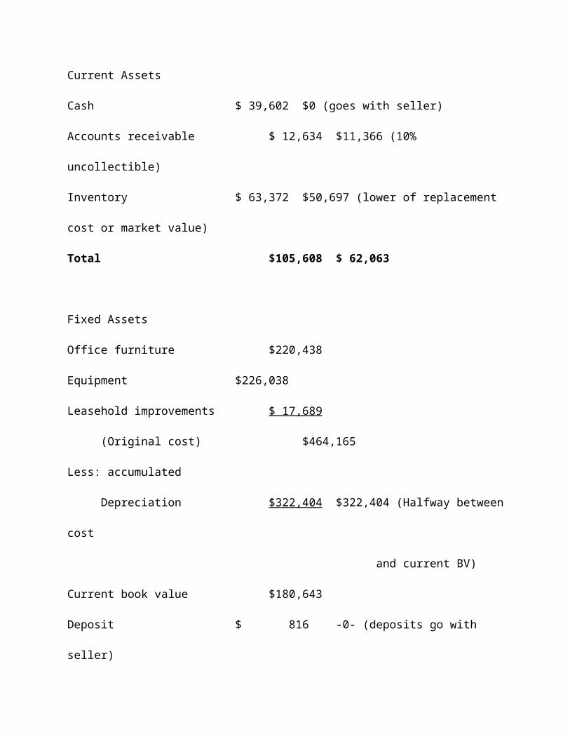
First, the tangible assets must be valued:

Balance Sheet

(Adjusted Values)

Current Assets

Cash $ 39,602 $0 (goes with seller)

Accounts receivable $ 12,634 $11,366 (10% uncollectible)

Inventory $ 63,372 $50,697 (lower of replacement cost or

market value)

Total $105,608 $ 62,063

Fixed Assets

Office furniture $220,438

Equipment $226,038

Leasehold improvements $ 17,689

(Original cost) $464,165

Less: accumulated

Depreciation $322,404 $322,404 (Halfway between cost

and current BV)

Current book value $180,643

Deposit $ 816 -0- (deposits go with seller)

Total $181,459 $322,404

Total tangible assets $384,467

The bottom line of our analysis is that the tangible assets have an estimated current FMV

of $384,467. If the business is being sold as an asset sale, the $11,366 value for the receivables

should be subtracted, giving us a total of $373,101. We will assume that the seller has agreed to

include these minimal receivables with the sale and use the higher asset figure. The more

significant the dollar value of the assets, the more important a professional appraisal would be. If

bank financing is involved, it is likely that formal appraisals will be required.

Next we need to determine a normalized operating profit. We will use only the current

period's income statement to estimate a normalized figure because the business has been

suffering from declining revenues and cash flows, leaving little reason to place a weight on these

previously higher numbers. Note that valuation transcends science and becomes an art precisely

because of such decisions. If the decline in sales is temporary and easily reversed, a higher figure

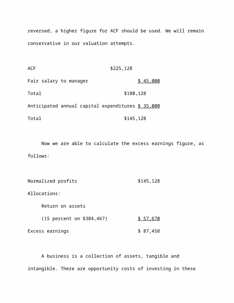
for ACF should be used. We will remain conservative in our valuation attempts.

ACF $225,128

Fair salary to manager $ 45,000

Total $180,128

Anticipated annual capital expenditures $ 35,000

Total $145,128

Now we are able to calculate the excess earnings figure, as follows:

Normalized profits $145,128

Allocations:

Return on assets

(15 percent on $384,467) $ 57,670

Excess earnings $ 87,458

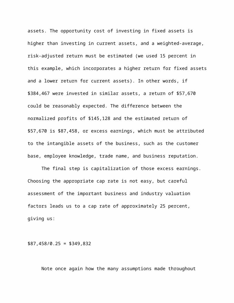
A business is a collection of assets, tangible and intangible. There are opportunity costs

of investing in these assets. The opportunity cost of investing in fixed assets is higher than

investing in current assets, and a weighted-average, risk-adjusted return must be estimated (we

used 15 percent in this example, which incorporates a higher return for fixed assets and a lower

return for current assets). In other words, if $384,467 were invested in similar assets, a return of

$57,670 could be reasonably expected. The difference between the normalized profits of

$145,128 and the estimated return of $57,670 is $87,458, or excess earnings, which must be

attributed to the intangible assets of the business, such as the customer base, employee

knowledge, trade name, and business reputation.

The final step is capitalization of those excess earnings. Choosing the appropriate cap rate

is not easy, but careful assessment of the important business and industry valuation factors leads

us to a cap rate of approximately 25 percent, giving us:

$87,458/0.25 = $349,832

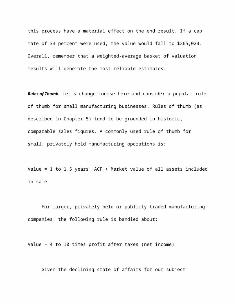
Note once again how the many assumptions made throughout this process have a material

effect on the end result. If a cap rate of 33 percent were used, the value would fall to $265,024.

Overall, remember that a weighted-average basket of valuation results will generate the most

reliable estimates.

Rules of Thumb. Let's change course here and consider a popular rule of thumb for small

manufacturing businesses. Rules of thumb (as described in Chapter 5) tend to be grounded in

historic, comparable sales figures. A commonly used rule of thumb for small, privately held

manufacturing operations is:

Value = 1 to 1.5 years' ACF + Market value of all assets included in sale

For larger, privately held or publicly traded manufacturing companies, the following rule

is bandied about:

Value = 4 to 10 times profit after taxes (net income)

Given the declining state of affairs for our subject business, we will use one year's ACF.

If there is a credible, realistic reason why the business has recently declined and could be quickly

turned around, a higher multiple could be justified. In our case, we will use a multiple of one, so

ACF = $225,128.

Turning to the assets, which have been valued at $384,467, we calculated the value of the

business as

ACF $225,128

+ Assets $384,467

= $609,595

What a difference from the excess earnings method! Let's reconsider our work so far.

Maybe we have overestimated the ACF. It looks solid, but one important change could be made

to bring this result more in line with that of the excess earnings method. If it is necessary, as we

assumed earlier, to devote $35,000 each year to replace the existing equipment to maintain the

future cash flows, the ACF should be reduced accordingly. Most business brokers do not make

this kind of adjustment (nor do they use the excess earnings method unless it is a larger small

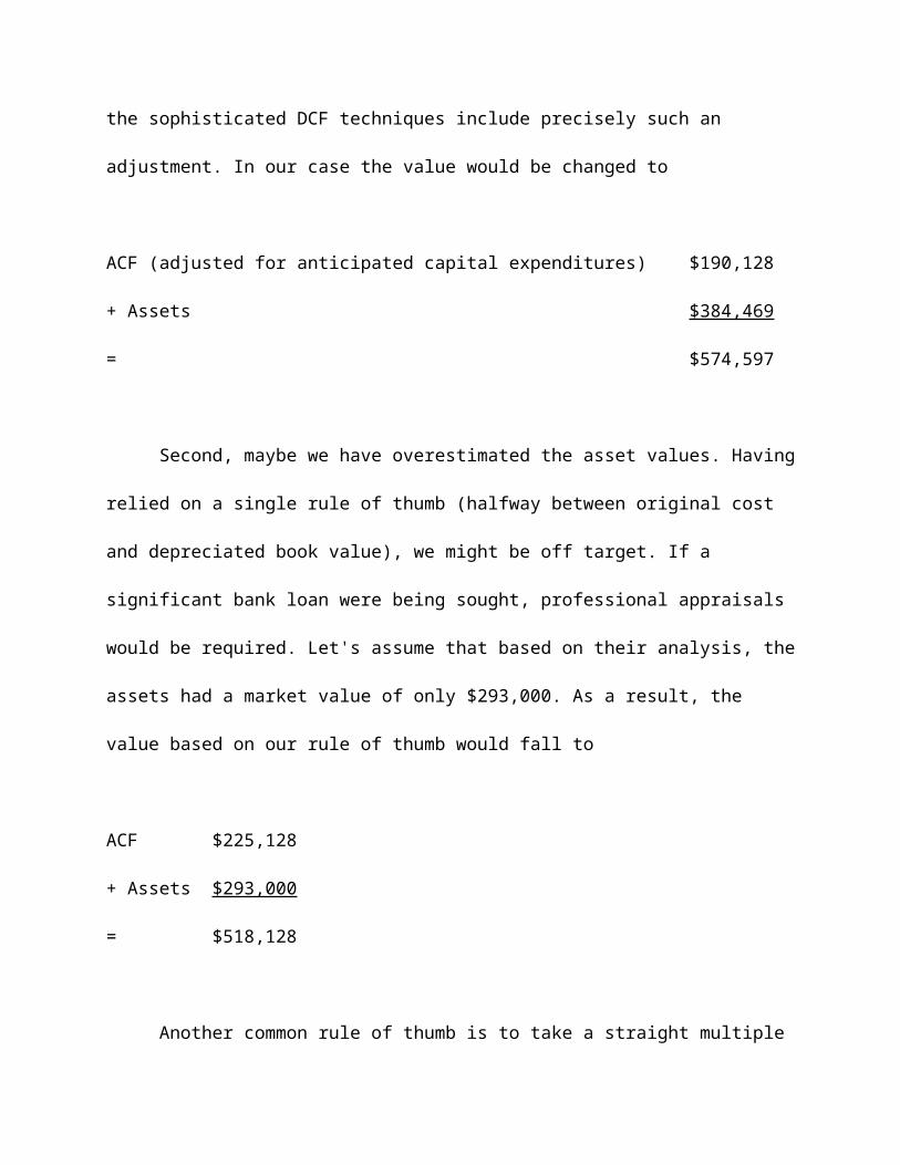
business), but the sophisticated DCF techniques include precisely such an adjustment. In our

case the value would be changed to

ACF (adjusted for anticipated capital expenditures) $190,128

+ Assets $384,469

= $574,597

Second, maybe we have overestimated the asset values. Having relied on a single rule of

thumb (halfway between original cost and depreciated book value), we might be off target. If a

significant bank loan were being sought, professional appraisals would be required. Let's assume

that based on their analysis, the assets had a market value of only $293,000. As a result, the value

based on our rule of thumb would fall to

ACF $225,128

+ Assets $293,000

= $518,128

Another common rule of thumb is to take a straight multiple of the ACF without regard to

asset values. Generally, a multiple of 1 to 3 is used, depending on the many factors that make

one business more attractive and secure than another. Manufacturing businesses normally enjoy

higher multiples than service businesses because of their large asset base. Given the downward

trend in sales and revenues, use of a multiple of only 2.5 might be justified.

Value = (2.5)(225,128) = $562,820

Value = (2.5)(190,128) = $475,320

Already we have values ranging from $349,832 to $609,595, and we are just getting

started.

Capitalization of Earnings Method. This method also relies exclusively on the capitalization of

historic earnings. The earnings base is different, and the value of tangible assets is basically

ignored. The first step, once again, is to calculate a normalized earnings base generated from the

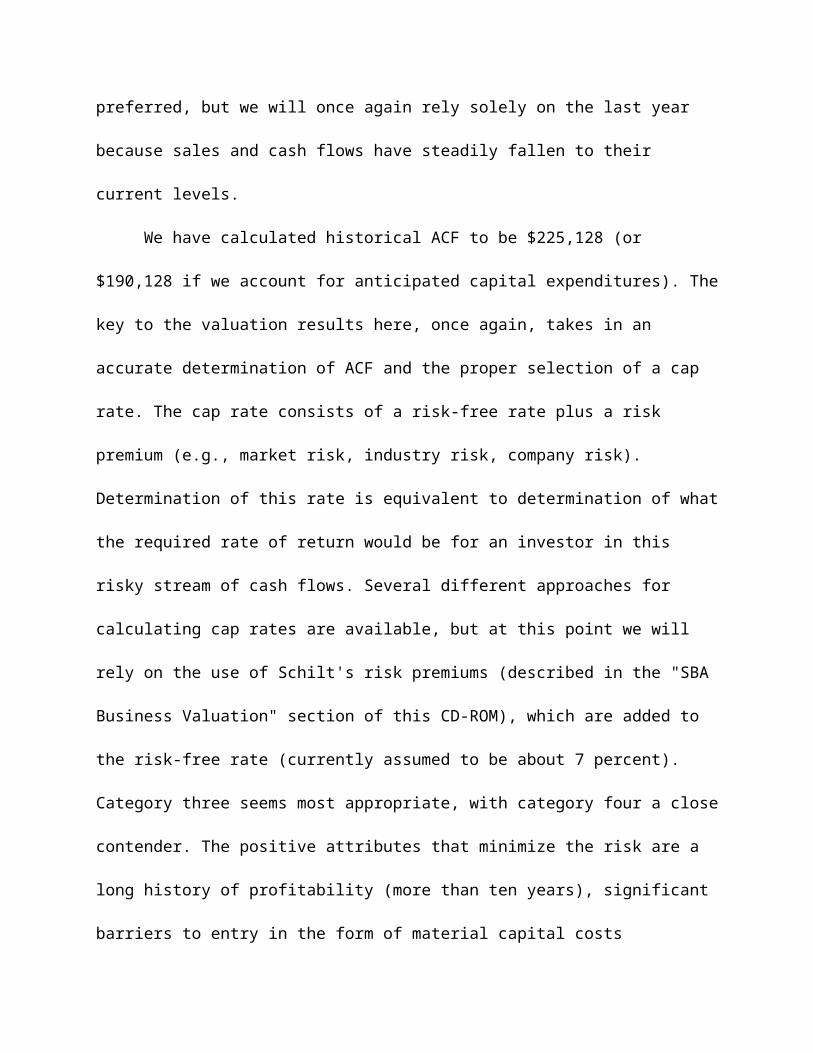
previous five years of financial results. A weighted average, with a greater weight on current

years, is preferred, but we will once again rely solely on the last year because sales and cash

flows have steadily fallen to their current levels.

We have calculated historical ACF to be $225,128 (or $190,128 if we account for

anticipated capital expenditures). The key to the valuation results here, once again, takes in an

accurate determination of ACF and the proper selection of a cap rate. The cap rate consists of a

risk-free rate plus a risk premium (e.g., market risk, industry risk, company risk). Determination

of this rate is equivalent to determination of what the required rate of return would be for an

investor in this risky stream of cash flows. Several different approaches for calculating cap rates

are available, but at this point we will rely on the use of Schilt's risk premiums (described in the

"SBA Business Valuation" section of this CD-ROM), which are added to the risk-free rate

(currently assumed to be about 7 percent). Category three seems most appropriate, with category

four a close contender. The positive attributes that minimize the risk are a long history of

profitability (more than ten years), significant barriers to entry in the form of material capital

costs (approximately $250,000), and the need for specialized skills. Ironically, this latter strength

turns out to be a weakness (increasing risk) to the extent that if one or two key employees were

to leave, business would suffer as the search for replacements took place. Assuming that the key

employees would sign a long-term employment contract (minimum of six months with at least

one month's notice required before leaving), this risk could be minimized, and category three

would seem appropriate. Category three requires the addition of 16 to 20 percent to the risk-free

rate of 7 percent, leaving a final rate of, say, 27 percent. The valuation results from here are quite

straightforward, as follows:

Value = $225,128/0.27 = $833,807

Value = $190,128/0.27 = $704,178

If employment contracts were not obtainable and the new owner did not have extensive

skills in this area, category four or five might apply. Consider the value based on cap rates of 31

or 34 percent.

Value = $225,128/0.31 = $726,219

Value = $190,128/0.31 = $613,316

Value = $225,128/0.34 = $662,141

Value = $190,128/0.34 = $559,200

This brings up an important and often overlooked point in business valuation. Businesses

have different values to different buyers. Depending on buyer backgrounds, a business venture

can be extremely risky or extremely safe. These differences must be considered during the

valuation process. There is no single valuation figure that applies to a given business.

Ability to Pay Method. This method is different from most others to the extent that you back into

the purchase price based on the anticipated cash flow and the desired payback period. Beginning

with our standard ACF ($225,128), we subtract the owner's required salary ($50,000), the

anticipated annual capital expenditures needed to maintain the cash flows ($35,000), and

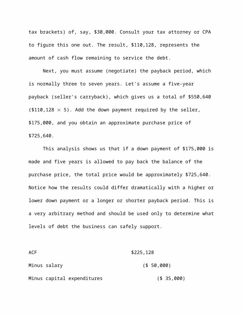
expected tax payments (varies from buyer to buyer depending on tax brackets) of, say, $30,000.

Consult your tax attorney or CPA to figure this one out. The result, $110,128, represents the

amount of cash flow remaining to service the debt.

Next, you must assume (negotiate) the payback period, which is normally three to seven

years. Let's assume a five-year payback (seller's carryback), which gives us a total of $550,640

($110,128 5). Add the down payment required by the seller, $175,000, and you obtain an

approximate purchase price of $725,640.

This analysis shows us that if a down payment of $175,000 is made and five years is

allowed to pay back the balance of the purchase price, the total price would be approximately

$725,640. Notice how the results could differ dramatically with a higher or lower down payment

or a longer or shorter payback period. This is a very arbitrary method and should be used only to

determine what levels of debt the business can safely support.

ACF $225,128

Minus salary ($ 50,000)

Minus capital expenditures ($ 35,000)

Minus taxes ($ 30,000)

Cash flow available to service debt $110,128

Assume 5-year pay back $550,640

Assume $175,000 down payment $175,000

Purchase price $725,640

Before completing our valuation analysis (ACF and adjusted book value approaches),

let's look at the average of results so far:

V1 = $349,832

V2 = $609,595

V3 = $574,597

V4 = $518,128

V5 = $562,820

V6 = $475,320

V7 = $833,807

V8 = $704,177

V9 = $726,219

V10 = $613,316

V11 = $662,141

V12 = $559,200

Vaverage = $599,096

Our average at this point is $599,096, which represents a value of approximately 2.66

times ACF.

DCF Method. Now we will attempt to value our business based on the DCF method, which is

forward-looking and relies on material estimates regarding the amount, timing, and risk of the

expected future cash flows. Specifically, the following areas must be credibly forecasted

(assuming the new owner is in control of the business):

- Sales, cost of goods sold, operating expenses (including owner's capital expenditures and

existing expenditures)

- Depreciation and amortization expenses (including capital expenditures)

- Interest expenses

- Additions to working capital

- Other future-related events

It is one thing to understand the current health of a company (based on historical data)

and quite another to predict the future under new ownership. Relevant historical data to be

analyzed include:

- Financial statements from the past five years

- Review of all product lines and services offered, summary of company history

- Complete list of assets included in sale

- Breakdown of inventory, accounts receivable, and accounts payable

- Important competitors, customers, suppliers, and employees

- Strengths, weaknesses, opportunities, and threats

- All leases, contractual commitments, and other likely financial obligations such as returns and

contingent liability

This review is critical for understanding the business in general as well as trying to

establish its value. Predicting or forecasting the future is based largely on understanding the past.

New ownership may lead to significant changes in both strategic and tactical plans, necessitating

adjustments to the pro forma financial statements and careful consideration of a number of key

areas, including the following:

- Plans to reduce costs

- Strategies to increase sales

- Potential acquisitions to spur growth

- Reduction of owner's compensation (salary plus benefits)

- Adjustments in accounting methods (including redepreciation of fixed assets)

- Projections of future, macroeconomic performance

All of these areas must be credibly analyzed and incorporated into future period

projections. There are different ways to use the DCF approach. Recent court cases have seen

greater reliance on this method as a preferred way to value businesses. The essence of this

method, once again, is to calculate the present value (PV) of all future cash flows accruing to the

owner.

The specific approach that we will use here is to add the PV of the expected cash flows to

the PV of the residual assets (assets minus liabilities) that will accrue to the owner at the time of

sale several years into the future.

The valuator has prepared the pro forma projections based on lengthy discussions with

the seller and the buyer. The seller knows the details of the business, and the buyer has specific

plans for the future regarding owner's compensation, advertising, purchasing, and new

equipment. Notice once again that the same business today will be worth differing amounts to

different buyers with different experience and different plans (i.e., investment value differs from

FMV). The important point to recognize is that you must carefully project the future sales and

expenses, putting great effort into these calculations, which at the same time will help the new

owner understand and run the business. The cash flow projections for this company should be

determined in a detailed manner supported with credible assumptions.

When applying DCF analysis, the valuator must analyze and determine the following:

- What measure of cash flow will you use?

- Will you include initial investments, cash infusions into working capital, replacements and

additions to fixed assets, and a terminal value upon sale many years into the future as part of

your bottom-line cash flow projections?

- How will you finance increased advertising expenditures, and how much will they increase

projected sales and profits?

- How much will sales and operating expenses increase?

- How much will interest expense be (what are the expected down payment and total purchase

price)?

- How risky are these anticipated cash flows (what discount rate is appropriate)?

These questions must be answered in a logical, consistent fashion to produce reliable

results. The pro forma cash flow analysis led to cash flow figures as follows for the next ten

years:

Year 1 Year 2 to 10

$212,000 8% growth each year

After the expected cash flows have been projected, they must be discounted back into

present value (PV). I have slightly modified the previously used cap rate (in the capitalization of

earnings method) to 30 percent, which was calculated using a build-up approach instead of

Schilt's risk premiums.

ACF PV

1 $212,000 $163,077

2 $228,960 $135,480

3 $247,276 $112,553

4 $267,059 $ 93,505

5 $288,424 $ 77,681

6 $311,498 $ 64,536

7 $336,417 $ 53,615

8 $363,331 $ 44,541

9 $392,397 $ 37,003

10 $423,789 $ 30,742

The PV of all future cash flows (using the ACF concept and ignoring working capital

infusions, capital replacements, and taxes) is therefore $812,733. If we accounted for capital

replacements and taxes or raised the discount rate, the valuation results would decline.

Adjusted Book Value Method. This method also is called the book value method, the net tangible

asset value method, the asset accumulation method, the sum of the assets method, or the

economic value of assets method. The essence of these methods is to determine the adjusted

book value of the business. Clearly, the idea that a business is worth its book value (A-L)is

questionable because the quirks of the accounting process and the diversion of book value from

true market value. Accordingly, the adjusted book value approach calls for proper adjustments to

be made for intangible assets such as goodwill and customer lists (see the discussion of

intangible assets in the "Accounting Primer" section of this CD-ROM), the economic

depreciation of fixed assets, appreciation in real estate values, and improperly stated inventory

amounts.

A critical choice to be made for most of these methods is whether to use market values or

liquidation values for the assets. Liquidation values are well below market values and would lead

to dramatically lower valuations. The decision is a function of the purpose of the valuation. If the

valuation concerns the potential purchase or sale of the company and the company is a viable

going concern generating profits, then the FMV standard should apply.

As always, a basket of valuation approaches is recommended for optimal results. Use of

the adjusted book value method alone is not advisable, except for perhaps newly established

businesses without a track record for sales and cash flow. This approach is also used in rare cases

in which the assets of the business will be liquidated piecemeal after acquisition (e.g.,

bankruptcy cases). This method almost always undervalues businesses that are generating profits

and cash flow.

As concerns our current business (High-Tech), the asset approaches do not seem to be

worthwhile, given the ten-year history of positive earnings. If we were to apply this method,

adjustments to all balance sheet accounts and a few amounts that do not show up on the balance

sheet would be necessary (e.g. goodwill, fully depreciated assets, and contingent liabilities). The

relevance of most if not all liability amounts disappears if the buyer is purchasing the assets only

(as opposed to a stock purchase).

The practical point is that almost every business, including companies that are losing

money, is worth at least the value of its assets (whether liquidation, market, or somewhere in

between). Even companies that generate negative valuation results because of negative cash flow

should be valued at least at their usable, marketable assets, both tangible and intangible.

Valuator's Conclusion. Placing a 50 percent weighting on the average result figured earlier

($599,096) and a 50 percent weighting on the DCF approach ($812,733), we might be

comfortable in stating that the current market value of this business is somewhere in between

these two numbers, or approximately $700,000 (which amounts to a multiple of ACF of

approximately 3).

Additional Author Comments

Go back and review the comments made at the beginning of this case study. Although the final

results appear to be reasonable, ask yourself how such an analysis would be received by another

valuator or a judge in a court of law. This case illustrates the importance of a logical, organized,

and easily understood format such as the ARM approach. Remember, business valuation takes

on meaning only in the heat of the battle. Bear in mind that your results probably will be

reviewed by another party, and you must be able to convincingly and credibly support your

findings (unless you are estimating value simply out of curiosity about your own business).