
6 Benchmarking and Reconciliation · benchmarking methods could help identify areas of research to...
41
6 Benchmarking and Reconciliation Benchmarking methods in the national accounts are used to derive quarterly series that are consistent with their corresponding annual benchmarks and, at the same time, preserve the short-term movements of quarterly economic indicators. Similarly, reconciliation methods may be necessary to adjust quarterly series that are subject to both annual and quarterly aggrega- tion constraints. is chapter presents benchmarking and reconciliation methods that are considered suit- able for QNA compilation. Practical guidance is also provided to address and resolve specific issues arising from the application of these methods in the national accounts. Introduction 1 Benchmarking deals with the problem of com- bining a series of high-frequency data (e.g., quarterly data) with a series of low-frequency data (e.g., an- nual data) for the same variable into a consistent time series. e two series may show different levels and movements, and need to be made temporally con- sistent. Because low-frequency data are usually more comprehensive and accurate than high-frequency ones, the high-frequency series is benchmarked to the low-frequency data. 2 is chapter discusses the use of benchmark- ing to derive quarterly national accounts (QNA) estimates that are consistent with annual national ac- counts (ANA) estimates. Annual estimates derived from the ANA system provide benchmark values for the QNA estimates. Usually, quarterly data sources rely on a more limited set of information than annual data. For this reason, quarterly data may present non- negligible differences in levels and movements with respect to annual data. Consequently, the annual data provide the most reliable information on the overall level and long-term movements for the national ac- counts variable, while the quarterly source data pro- vide the only available explicit information about the short-term movements in the series. Benchmarking is a necessary step to combine the quarterly pattern in the indicator with the annual benchmarks of the ANA variable. 3 Benchmarking techniques help improve the quality of QNA series by making them consistent with ANA benchmarks and coherent with the short-term evolution of quarterly economic indicators. However, the accuracy of QNA data ultimately depends on the accuracy of the annual benchmarks and quarterly in- dicators. A prerequisite of quality for the QNA data is to rely on information that measures precisely what is happening in the economy, both in normal times and during periods of sudden and unexpected changes. e role of benchmarking is to combine in the best possible way the annual and quarterly information at disposal. 4 While quarterly-to-annual benchmarking is the most relevant case in QNA compilation, benchmark- ing can also be conducted to adjust national accounts data available at other frequencies. For example, a monthly activity indicator can be benchmarked to a quarterly GDP series (monthly-to-quarterly bench- marking). Benchmarking can also be useful for ANA data, when preliminary annual accounts need to be adjusted to meet comprehensive benchmark revisions of national accounts available every five or ten years. Even though this chapter is focused on the quarterly- to-annual benchmarking, principles and methods outlined here apply to benchmarking of any other high-frequency to low-frequency data. 5 For some variables, quarterly data sources are used directly to derive the annual data of the ANA system. In this situation, annual totals automatically meet their quarterly counterparts and the benchmark- ing step is unnecessary. is happens, for instance, when annual data are derived from the aggregation of monthly or quarterly information that is not subject
Transcript of 6 Benchmarking and Reconciliation · benchmarking methods could help identify areas of research to...

6 Benchmarking and Reconciliation
Benchmarking methods in the national accounts are used to derive quarterly series that are consistent with their corresponding annual benchmarks and, at the same time, preserve the short-term movements of quarterly economic indicators. Similarly, reconciliation methods may be necessary to adjust quarterly series that are subject to both annual and quarterly aggrega-tion constraints. This chapter presents benchmarking and reconciliation methods that are considered suit-able for QNA compilation. Practical guidance is also provided to address and resolve specific issues arising from the application of these methods in the national accounts.
Introduction1 Benchmarking deals with the problem of com-
bining a series of high-frequency data (e.g., quarterly data) with a series of low-frequency data (e.g., an-nual data) for the same variable into a consistent time series. The two series may show different levels and movements, and need to be made temporally con-sistent. Because low-frequency data are usually more comprehensive and accurate than high-frequency ones, the high-frequency series is benchmarked to the low-frequency data.
2 This chapter discusses the use of benchmark-ing to derive quarterly national accounts (QNA) estimates that are consistent with annual national ac-counts (ANA) estimates. Annual estimates derived from the ANA system provide benchmark values for the QNA estimates. Usually, quarterly data sources rely on a more limited set of information than annual data. For this reason, quarterly data may present non-negligible differences in levels and movements with respect to annual data. Consequently, the annual data provide the most reliable information on the overall level and long-term movements for the national ac-counts variable, while the quarterly source data pro-vide the only available explicit information about the
short-term movements in the series. Benchmarking is a necessary step to combine the quarterly pattern in the indicator with the annual benchmarks of the ANA variable.
3 Benchmarking techniques help improve the quality of QNA series by making them consistent with ANA benchmarks and coherent with the short-term evolution of quarterly economic indicators. However, the accuracy of QNA data ultimately depends on the accuracy of the annual benchmarks and quarterly in-dicators. A prerequisite of quality for the QNA data is to rely on information that measures precisely what is happening in the economy, both in normal times and during periods of sudden and unexpected changes. The role of benchmarking is to combine in the best possible way the annual and quarterly information at disposal.
4 While quarterly-to-annual benchmarking is the most relevant case in QNA compilation, benchmark-ing can also be conducted to adjust national accounts data available at other frequencies. For example, a monthly activity indicator can be benchmarked to a quarterly GDP series (monthly-to-quarterly bench-marking). Benchmarking can also be useful for ANA data, when preliminary annual accounts need to be adjusted to meet comprehensive benchmark revisions of national accounts available every five or ten years. Even though this chapter is focused on the quarterly-to-annual benchmarking, principles and methods outlined here apply to benchmarking of any other high-frequency to low-frequency data.
5 For some variables, quarterly data sources are used directly to derive the annual data of the ANA system. In this situation, annual totals automatically meet their quarterly counterparts and the benchmark-ing step is unnecessary. This happens, for instance, when annual data are derived from the aggregation of monthly or quarterly information that is not subject
6240-082-FullBook.indb 86 10/18/2017 6:08:58 PM

Benchmarking and Reconciliation 87
to future revisions. In a few cases, quarterly data may be superior and so may be used to replace the annual data. One instance is annual deflators that are best built up from quarterly data as the ratio between the annual sums of the quarterly current and constant price data (as explained in Chapter 8 ). Another example is when annual data are derived using nonstandard account-ing practices. More generally, annual data should be quality assured prior to any benchmarking. Compil-ers should not adjust good-quality quarterly data to lower-quality annual data. However, such cases are infrequent and the standard practice in the QNA is to use quarterly data as indicators to break down more comprehensive and accurate annual figures.
Objectives of Benchmarking6 In the QNA, benchmarking serves two purposes:
· quarterly distribution (or interpolation)1 of an-nual data to construct time series of bench-marked QNA estimates (“back series”) and
· quarterly extrapolation to derive the QNA esti-mates for quarters for which ANA benchmarks are not yet available (“forward series”).
7 Ideally, both distribution and extrapolation of QNA series must be based on quarterly indicators that are statistically and economically correlated to the annual variables considered.2 The term “indicator” is adopted in a broad sense in this context. It indicates either a sub-annual measurement of the same target variable or a proxy variable that closely approximates the (unknown) quarterly behavior of the target vari-able. An example in the first group is the quarterly value of merchandise imports (or exports) from for-eign trade statistics as a short-term approximation of imports (exports) of goods at current prices in the ANA; in the second group, the quarterly industrial pro-duction index could be used as a proxy of the volume measure of the annual gross value added of manufac-turing. When such indicators are absent, it is advisable
1 Distribution is associated with flow series, when the annual series is calculated as the sum (or the average) of the quarterly data. Interpolation usually applies to stock series, when quarterly series needs to match the annual value in a specified time of the year (e.g., January 1st). As this manual focuses on quarterly GDP, which is a flow series, the term “quarterly distribution” will be used in the chapter to indicate quarterly-to-annual benchmarking.2 More details on the selection process of indicators are given in Chapter 5.
to look at other indicators that are closely related to the concept measured by the variable to be estimated or consider the movements of related QNA aggregates. Application of mathematical procedures to distribute annual totals into quarters without the use of related quarterly indicators should be minimized (see para-graphs 6.75–77 for further details on when this ap-proach can be considered feasible). To be relevant for the user, short-term movements of the QNA should closely reflect what is happening in the economy.
8 The format and level of the indicators should not influence the benchmarking results of the QNA.3 In the benchmarking framework, the objective is to combine the quarterly movements of the indicator with the annual levels of the ANA variables. The quar-terly indicator may be in the form of index numbers (value, volume, or price) with a reference period that may differ from the base period in the QNA, may be expressed in physical units, may be expressed in mon-etary terms, or may be derived in nominal terms as the product of a price index and a volume index. The in-dicator serves only to determine the quarterly move-ments in the estimates (or quarter-to-quarter change), while the annual data determine the overall level and long-term trend. However, the annual movements of the indicator are used to assess whether the indicator is a good approximation of the annual movements of the ANA target variable. Therefore, the annual rela-tionship between the ANA variable and the quarterly indicator directly affects the preservation of move-ments and the accuracy of extrapolation.
9 In this chapter, quarterly distribution and ex-trapolation are unified into one common benchmark-to-indicator (BI) ratio framework for converting quarterly indicator series into QNA variables. The relationship between the annual data and the quar-terly indicator can be assessed by looking at the move-ments of the annual BI ratio: namely, the ratio of the annual benchmark to the sum of the four quarters of the indicator. In mathematical terms, the annual BI ratio can be expressed as follows:
AI
n
n for n y=1,..., (1)
3 For this reason, benchmarking methods should produce results that are invariant to level difference in the same indicator. The proportional benchmarking methods discussed in this chapter satisfy this requirement.
6240-082-FullBook.indb 87 10/18/2017 6:08:58 PM

Quarterly National Accounts Manual 201788
where
An is the ANA target variable for a generic year n;
In is the annual sum of the quarterly observations of the
indicator for the same year n, that is, I In tt n
n
== −∑
4 3
4
;
and
y is the time index of the last available year. 4
When the BI ratio changes over time, it signals dif-ferent patterns between the indicator and the annual data; instead, a constant annual BI ratio means that the two variables present the same rates of change.5 As a result, movements in the annual BI ratio (equa-tion (1)) can help identify the quality of the indicator series in tracking the movements of the ANA variable over the years. The benchmarking methods consid-ered in this chapter distribute and extrapolate the an-nual BI ratio on a quarterly basis.
10 In the QNA, the main objectives of benchmark-ing are the following:
· to estimate quarterly data that are temporally consistent with the ANA data: that is, to ensure that the sum (or the average) of the quarterly data is equal to the annual benchmark;
· to preserve as much as possible the quarterly movements in the indicator under the restric-tions provided by the ANA data; and
· to ensure, for forward series, that the sum of the four quarters of the current year is as close as possible to the unknown future ANA data.
11 The ideal benchmarking method for QNA should be able to meet all three objectives. Quarterly movements in the indicator need to be preserved because they provide the only available explicit in-formation on a quarterly basis that are deemed to approximate the unknown quarterly pattern of QNA series. This strict association with the indicator series applies to both the back series and the forward series. In addition, the forward series should be as close as possible to the annual benchmark when it becomes
4 In this chapter, index n denotes the years and index t denotes the quarters. The quarterly index of the four quarters of a generic year n are identified by 4n – 3 (first quarter), 4n – 2 (second quarter), 4n – 1 (third quarter), and 4n (fourth quarter). As an example, t 5 1, 2, 3, 4 for the first year (n 5 1).5 When the BI ratio is constant, any level difference between the annual sum of the indicator and the annual data can be removed by simply multiplying the indicator series by the constant BI ratio.
available. These two requirements, however, might be at odds: in some cases, quarterly extrapolation should deviate from the quarterly movements in the origi-nal indicator in order to obtain better estimate of the ANA variable for the next year.
12 Benchmarking can also be useful to identify and correct distortions in the national accounts com-pilation, and reduce revisions in the preliminary esti-mates of QNA. Bad-quality results of benchmarking can highlight inconsistencies between quarterly and annual sources as soon as they happen. The use of benchmarking methods could help identify areas of research to improve the consistency between annual and quarterly accounts data. In seasonal adjustment, benchmarking can detect when seasonally adjusted re-sults drift away from unadjusted data (see Chapter 8).
Overview of Benchmarking Methods13 The pro rata method, which is a simple method
of benchmarking, should be avoided. The pro rata method distributes the temporal discrepancies—the differences between the annual sums of the quarterly estimates and the annual data—in proportion to the value of the indicator in the four quarters of each year. The next section shows that the pro rata approach produces unacceptable discontinuities from one year to the next (the so-called step problem) and therefore does not preserve the movements in the indicator from the fourth quarter of one year to the first quarter of the next. Techniques that introduce breaks in the time series seriously hamper the usefulness of QNA by distorting economic developments and possible turning points. They also thwart forecasting and con-stitute a serious impediment for seasonal adjustment and trend analysis.
14 To avoid the step problem, proportional bench-marking methods with movement preservation of indicators should be used to derive QNA series. The preferred solution is the proportional Denton method. The proportional Denton method keeps the quarterly BI ratio as stable as possible subject to the restrictions provided by the annual data. Paragraph 6.31 shows that minimizing the movements of the quarterly BI ratio correspond to preserving very closely the quar-terly growth rates of the indicator.
15 In extrapolation, the proportional Denton method may yield inaccurate results when the most
6240-082-FullBook.indb 88 10/18/2017 6:08:59 PM

Benchmarking and Reconciliation 89
recent annual BI ratios deviate from the historical BI average. This happens when the annual movement in the indicator diverges from the annual movement in the ANA variable for the most recent years. This problem can be circumvented using an enhancement for extrapolation to the proportional Denton tech-nique. The enhanced version provides a convenient way of adjusting for a temporary bias6 and still maxi-mally preserving the short-term movements in the source data. However, the enhanced solution requires an explicit forecast of the next annual BI ratio to be provided by the user.
16 As an alternative to the Denton method, the proportional Cholette–Dagum method with first-order autoregressive (AR) error can be used to obtain extrapolations adjusted for the historical bias.7 This method is derived as a particular case of the more general Cholette–Dagum regression-based bench-marking model (illustrated in Annex 6.1). As shown in paragraph 6.56, under specific conditions for the value of the AR coefficient, the proportional Cholette–Dagum method with AR error provides movements in the back series that are sufficiently close to the in-dicator (and similar results to the Denton method). More importantly, it returns extrapolations for the forward series that takes into account the historical bias with the indicator.
17 The chapter tackles more specific issues arising from the application of benchmarking in the compi-lation of QNA. The Boot–Feibes–Lisman smoothing method—a method equivalent to the proportional Denton method with a constant indicator—provides an appropriate solution for benchmarking ANA vari-ables without the use of a related indicator. Practical solutions are given to solve difficult benchmarking cases, such as short series, series with breaks, series requiring specific seasonal effects, or series presenting negative or zero values. The chapter also discusses the impact on benchmarking when either (preliminary) annual benchmarks or (preliminary) quarterly values of the indicator are revised.
18 Finally, the chapter extends the benchmarking methodology to solve reconciliation problems in the
6 Instead, when the bias in the movements is permanent, the basic proportional Denton method may still provide accurate extrapolations. 7 In a first-order autoregressive model, the current value of the error is linearly dependent to the value of the previous period.
QNA. Reconciliation is required to restore consis-tency in quarterly series that are subject to both an-nual and quarterly aggregation constraints. The main difference with benchmarking is that the reconciled estimates have to satisfy both annual benchmarks and quarterly constraints. As an example, quarterly value added by institutional sector may be required to be in line with ANA estimates by institutional sector and independently derived quarterly value added for the total economy.
19 The multivariate proportional Denton method is recommended for reconciling QNA series subject to both ANA benchmarks and quarterly aggregates. However, when the number of variables is large, the multivariate solution could be computationally chal-lenging. To avoid this complication, the following two-step procedure is suggested as a close approxima-tion of the multivariate Denton approach:
· use the proportional Denton method to bench-mark each quarterly indicator to the correspond-ing ANA variable and
· use a least-squares balancing procedure to rec-oncile one year at a time the benchmarked series obtained at the first step with the given annual and quarterly constraints of that year.
20 Benchmarking and reconciliation techniques should be an integral part of the compilation process. These techniques are helpful to convert short-term in-dicators into estimates of QNA variables that are con-sistent with the ANA system. While benchmarking and reconciliation techniques presented in this chapter are technically complicated, it is important to emphasize that shortcuts generally will not be satisfactory unless the indicator shows almost the same trend as the bench-mark. The weaker the indicator is, the more important it is to use proper benchmarking and reconciliation techniques. While there are some difficult conceptual issues that need to be understood before setting up a new system, the practical operation of benchmark-ing and reconciliation are typically automated and are not problematic or time consuming using computers nowadays available. In the initial establishment phase, the issues need to be understood and the processes au-tomated as an integral part of the QNA production sys-tem. Thereafter, the techniques will improve the data and reduce future revisions without demanding time and attention of the QNA compilers.
6240-082-FullBook.indb 89 10/18/2017 6:08:59 PM

Quarterly National Accounts Manual 201790
21 Box 6.1 presents a brief overview of the bench-marking software available at the time of preparing this manual. Countries introducing QNA or improv-ing their benchmarking techniques may find it worth-while to obtain existing software for direct use or adaptation to their own processing systems. Alterna-tively, Annex 6.1 provides the algebraic solution (in matrix notation) of the proportional Denton method and the proportional Cholette–Dagum method. This formal presentation can facilitate the implementation of the two benchmarking solutions in any computing software.
The Pro Rata Distribution and the Step Problem
22 The aim of this section is to illustrate the step problem created by pro rata distribution and extend the pro rata approach to cover extrapolation from the last available benchmark. The ratio of the QNA benchmarked estimates to the indicator (the quarterly BI ratio) implied by the pro rata distribution method shows that this method introduces unacceptable dis-continuities into the time series. Also, viewing the quarterly BI ratios implied by the pro rata distribution method together with the quarterly BI ratios implied by the basic extrapolation with an indicator technique
shows how distribution and extrapolation with indi-cators can be put into the same BI framework. Be-cause of the step problem, the pro rata distribution technique is not acceptable.
23 In the context of this chapter, distribution refers to the allocation of an annual total of a flow series to its four quarters. A pro rata distribution splits the an-nual total according to the proportions indicated by the four quarterly observations. A numerical example is shown in Example 6.1 and Figure 6.1.
24 In mathematical terms, pro rata distribution can be formalized8 as follows:
X = I AIt t
n
n⋅
for n y=1,..., and t n n= −4 3 4,..., (2)
where
Xt is the level of the QNA estimate for quarter t,
It is the level of the quarterly indicator for quarter t
An is the level of the ANA estimate for year n,
In is the annual aggregation (sum or average) of the quarterly values of the indicator for year n,
8 Unless otherwise specified, in this chapter, the annual bench-marks are denoted with An, the quarterly indicator series with It , and the quarterly benchmarked series with Xt .
Box 6.1 Software for Benchmarking
The benchmarking methods presented in this chapter are available in some commercial and open-source software. Com-piling agencies using a specific package for QNA compilation should consult the technical guide to see if built-in bench-marking functions are available. If not, an Internet search can reveal if a plug-in or toolbox containing benchmarking routines is available for the specific package.
At the time of writing, compiling agencies may also consider two off-the-shelf solutions that have been specifically designed for the production of QNA and other official statistics:
• XLPBM (IMF). XLPBM is an add-in function to Microsoft Excel for benchmarking quarterly series to annual series using the proportional Denton method and the proportional Cholette–Dagum method with first-order autore-gressive error. It also implements the enhanced solution of the Denton method. It has been developed by the IMF Statistics Department to assist member countries within its technical assistance and training program. It is particularly suited for QNA compilation systems based on spreadsheets. It can be downloaded from the QNA manual webpage on IMF.org.
• JDemetra+ (National Bank of Belgium, Eurostat). JDemetra+ contains a plug-in offering several options for temporal disaggregation and benchmarking. The Denton and Cholette–Dagum methods are provided, as well as a generalization of the Denton multivariate case. It also implements regression-based methods such as Chow–Lin, Fernandez, and Litterman. It can deal with any valid combination of frequencies. For more information on JDemetra+ for seasonal adjustment, see Box 7.1.
Compiling agencies may also choose to implement benchmarking techniques in their preferred computing environment. Annex 6.1 offers a matrix formulation of the Denton and Cholette–Dagum benchmarking solutions. Both methods can easily be coded in any programming language that offers matrix algebra operations.
6240-082-FullBook.indb 90 10/18/2017 6:09:00 PM

Benchmarking and Reconciliation 91
Example 6.1 Pro Rata Method and the Step Problem
Indicator Pro Rata Method
Indicator Quarter-to- Quarter Rate
of Change (%)
Year-on- Year
Rate of Change
(%)
Annual Data
Annual BI Ratio
Benchmarked Data Quarter-to- Quarter Rate
of Change (%)
Year-on- Year
Rate of Change
(%) (1) (2) (3)=(2)/(1) (1) × (3) = (4)
q1 2010 99.4 99.4 × 2.5000 = 248.5
q2 2010 99.6 0.2 99.6 × 2.5000 = 249.0 0.2
q3 2010 100.1 0.5 100.1 × 2.5000 = 250.3 0.5
q4 2010 100.9 0.8 100.9 × 2.5000 = 252.3 0.8
2010 400.0 1,000.0 2.5000 1,000.0
q1 2011 101.7 0.8 2.3 101.7 × 2.5329 = 257.6 2.1 3.7
q2 2011 102.2 0.5 2.6 102.2 × 2.5329 = 258.9 0.5 4.0
q3 2011 102.9 0.7 2.8 102.9 × 2.5329 = 260.6 0.7 4.1
q4 2011 103.8 0.9 2.9 103.8 × 2.5329 = 262.9 0.9 4.2
2011 410.6 2.7 1,040.0 2.5329 1,040.0 4.0
q1 2012 104.9 1.1 3.1 104.9 × 2.4884 = 261.0 −0.7 1.3
q2 2012 106.3 1.3 4.0 106.3 × 2.4884 = 264.5 1.3 2.2
q3 2012 107.3 0.9 4.3 107.3 × 2.4884 = 267.0 0.9 2.4
q4 2012 107.8 0.5 3.9 107.8 × 2.4884 = 268.2 0.5 2.0
2012 426.3 3.8 1,060.8 2.4884 1,060.8 2.0
q1 2013 107.9 0.1 2.9 107.9 × 2.4884 = 268.5 0.1 2.9
q2 2013 107.5 −0.4 1.1 107.5 × 2.4884 = 267.5 −0.4 1.1
q3 2013 107.2 −0.3 −0.1 107.2 × 2.4884 = 266.8 −0.3 −0.1
q4 2013 107.5 0.3 −0.3 107.5 × 2.4884 = 267.5 0.3 −0.3
2013 430.1 0.9 — — 1,070.3 0.9
The Annual Data and the Quarterly Indicator In this example, we assume that the annual data are expressed in monetary terms and the quarterly indicator is an index with 2010 = 400. The annual data and the quarterly indicator show different movements in 2011 and 2012. The quarterly indicator shows a stable, smooth upward trend since 2010, with annual growth rates of 2.7 and 3.8 percent in 2011 and 2012, respectively. The annual data are characterized by a much stronger growth in 2011 than in 2012 (4.0% compared with 2.0%).
Pro Rata Distribution The annual BI ratio for 2010 (2.5) is calculated by dividing the annual value (1,000) by the annual sum of the index (400.0). This ratio is then used to derive the benchmarked estimates for the individual quarters of 2010. For example, the benchmarked estimate for q1 2010 is 248.5: that is, 99.4 times 2.5.
The Step Problem Observe that quarter-to-quarter rates are different only in the first quarters: +2.1% in the benchmarked data versus +0.8% in the indicator in q1 2011 and −0.7% versus +1.1% in q1 2012. These discontinuities (or steps) are caused by the different pace of growth of the two series, which causes sudden changes of the annual BI ratios in the years 2011 and 2012.
Extrapolation The 2013 indicator data are linked to the benchmarked data for 2012 by carrying forward the BI ratio for the year 2012 (2.4884). For instance, the extrapolation for q3 2013 (266.8) is derived as 107.2 times 2.4884. Note that all extrapolated quarters present the same quarter-to-quarter rates and year-on-year rates of the indicator. In addition, the annual rate of change is the same (0.9%).
(These results are illustrated in Figure 6.1. Rounding errors in the table may occur.)
6240-082-FullBook.indb 91 10/18/2017 6:09:00 PM

Quarterly National Accounts Manual 201792
Figure 6.1 Pro Rata Method and the Step Problem
245.0
250.0
255.0
260.0
265.0
270.0
98.0
100.0
102.0
104.0
106.0
108.0
2010 2011 2012 2013
Indicator (left-hand axis) Benchmarked Data with Pro Rata Method (right-hand axis)
Back Series Forward Series
In this example, the step problem shows up as an increase in the benchmarked series from q4 2010 to q1 2011 and as a subsequent drop from q4 2011 to q1 2012. Both movements are not matched by similar movements in the indicator.
Benchmark-to-Indicator Ratio
It is easier to recognize the step problem from charts of the BI ratio. It shows up as abrupt upward or downward steps in the BI ratios between q4 of one year and q1 of the next year. In this example, the step problem shows up as a large upward jump in the BI ratio between q4 2010 and q1 2011 and a subsequent drop between q4 2011 and q1 2012.
2.46
2.48
2.50
2.52
2.54
2.56
2010 2011 2012 2013
The Indicator and the Derived Benchmarked Series(The corresponding data are given in Example 6.1)
6240-082-FullBook.indb 92 10/18/2017 6:09:00 PM

Benchmarking and Reconciliation 93
n is the temporal index for the years,
y is the last available year, and
t is the temporal index for the quarters.
Equation (2) derives the QNA estimate by raising each quarterly value of the indicator It by the corre-sponding annual BI ratio A In n( ).
25 The step problem arises because of discontinui-ties in the annual BI ratio between years. If an indi-cator shows different annual growth rates than the annual benchmark, as in Example 6.1, then the BI ratio will move from one year to the next. When the annual BI ratio is used to elevate the indicator’s value for all the quarters, the entire difference in the quar-terly growth rates is put into the first quarter, while other quarterly growth rates are left unchanged.9 The significance of the step problem depends on the size of variations in the annual BI ratio.
26 Extrapolation with an indicator refers to using the movements in the indicator to update the QNA time series with estimates for quarters for which no annual data are yet available (the forward series). A numerical example is shown in Example 6.1 and Figure 6.1.
27 In mathematical terms, extrapolation with an indicator can be formalized using the same BI ratio presentation used for the distribution case:
X = IAIt t
y
y⋅
for t y y y y= + + + +4 1 4 2 4 3 4 1, , , ( ) (3)
where y indicates the year with the last available an-nual benchmark and extrapolations are needed for the quarterly values of the year y+1. It is assumed that the indicator is available for all the quarters of year y+1.
28 When equation (3) is applied, quarterly growth rates in the forward series reproduce exactly the quar-terly growth rates in the indicator in year y+1. This can be shown by dividing equation (3) for two adjacent quar-ters: the common BI ratio for year y in the right-hand side of equation (3) cancels out and the remaining ratios
4
4 1
4
4 11y k
y k
y k
y k
XX
= II
k+
+ −
+
+ −
=for ,, , ,2 3 4
9 In addition, the distributed series with the pro rata method pres-ents year-on-year growth rates (i.e., one quarter compared with the corresponding quarter of the previous year) that differ from those of the indicator in all the quarters.
show that the QNA series (equation (3)) present the same quarter-to-quarter rates of the indicator. Simi-larly, it can be shown that the QNA series has the same year-on-year growth rates of the indicator in the ex-trapolated quarters. Although in general these features may look like desirable properties, the extrapolated series might need to deviate from the movements of the indicator to match different annual movements in the ANA series for the next year.
29 In summary, pro rata distribution calculates the back series by using the corresponding BI ratios for each year where ANA benchmark is available as adjustment factors to scale up or down the indicator. The forward series is calculated by carrying forward the last annual BI ratio. This method is unacceptable for QNA benchmarking because it could introduce a step in the first quarter of the year, thus violating the stated objective of preserving the original move-ments in the indicator. The next section illustrates proportional benchmarking methods that are de-signed to preserve the movements in the indicator in all quarters.
Proportional Benchmarking Methods with Movement Preservation
30 From a quarterly perspective, the main objec-tive of benchmarking is to preserve the quarterly movements in the indicator. The most common mea-surement of movement in quarterly (seasonally ad-justed) series is the quarter-to-quarter (or quarterly) growth rate, which is measured by the ratio of the level of one quarter (It) to the level of the previous quarter It−( )1 .10 Another common way of measuring movements on quarterly (unadjusted) series is with year-on-year growth rates: the ratio of the level of one quarter (It) to the level of the same quarter in the previous year It−( )4 . Year-on-year quarterly growth rates are useful in benchmarking, because they can be directly related to the annual growth11 computed from the ANA series.
31 Ideally, the benchmarked series should maxi-mally preserve the quarterly growth rates in the
10 For example, if the ratio I It t/ -1 is 1.021, the indicator has increased by 2.1 percent in quarter t compared with the previous quarter t-1.11 Approximately, the annual average of year-on-year rates from a quarterly series returns the annual growth computed from the annually aggregated quarterly variable.
6240-082-FullBook.indb 93 10/18/2017 6:09:02 PM

Quarterly National Accounts Manual 201794
indicator subject to the constraints given by the an-nual benchmarks. In mathematical terms, this state-ment can be formulated as the minimization of the objective (penalty) function:12
minX
t
t
t
tt
q
t
XX
II− −=
−
∑
1 12
2
(4)
subject to the annual constraints
X A n yt nt n
n
= == −∑ for 1
4 3
4
, ..., , (5)
where
q is the last quarter for which quarterly source data are available, denoting either the fourth quarter of the last available year (q y= 4 ) in case of a distribution prob-lem or any subsequent quarter (q y> 4 ) for a problem with extrapolation.
Solving problem (4) subject to (5) corresponds to finding the quarterly (unknown) values Xt (i.e., the QNA series) that match the required annual bench-marks and present growth rates that are as close as possible to the growth rates of the indicator. Problem (4) is also known as growth rate preservation (GRP) function.
32 Despite being an ideal criterion for benchmark-ing from a theoretical viewpoint, the GRP problem (4) is a rational function of the target values and as such can only be minimized using nonlinear optimization algorithms.13 The implementation of these algorithms requires advanced knowledge of optimization theory and use of commercial software (see Annex 6.1 for ref-erence). Furthermore, these algorithms may be char-acterized by slow convergence and possible troubles in finding actual minima of the objective function. For this reason, GRP-based benchmarking proce-dures are considered impractical for QNA purposes.
33 The next section introduces the proportional Denton method, which is a close linear approximation of the GRP function and obtains the benchmarked se-ries using simple matrix algebra operations.
12 The quadratic expression in equation treats positive and nega-tive differences symmetrically and assigns proportionally higher weights to large differences than small ones.13 Formula presents the benchmarked values at the denominator and therefore is a nonlinear function of the benchmarked series.
The Proportional Denton Method
34 The proportional Denton benchmarking tech-nique keeps the ratio of the benchmarked series to the indicator (i.e., the quarterly BI ratio) as constant as possible subject to the constraints provided by the an-nual benchmarks. A numerical illustration of its op-eration is shown in Example 6.2 and Figure 6.2.
35 Using the same notation of equations (4) and (5), the proportional Denton technique can be expressed as the constrained minimization problem:14
minX
t
t
t
tt
q
t
XI
XI
−
−
−=∑ 1
1
2
2
(6)
subject to
X A n yt nt n
n
= == −∑
4 3
4
1for , ..., (7)
36 The individual term of the penalty function (6) minimized by the proportional Denton method (also known as proportional first difference variant of the Denton method) —is the first difference of the quar-terly BI ratio. With the Denton method, movement preservation is achieved by distributing the quarterly BI ratios smoothly from one quarter to the next under the annual restrictions (equation (7)). Implicitly, the quarterly benchmarked series will present growth rates similar to those of the indicator. It can be shown that function (6) approximates very closely the ideal GRP function (4). More importantly, the constrained minimization problem is a linear function of the ob-jective values (Xt only appears in the numerator). The first-order conditions for a minimum permits to de-rive a closed-form solution of the problem, and the benchmarked series can be calculated using standard matrix algebra operations (see Annex 6.1).
37 Under the BI framework, the proportional Den-ton technique implicitly constructs from the annual observed BI ratios a time series of quarterly BI ratios
14 This presentation deviates from Denton’s original proposal by omitting the requirement that the value for the first period be predetermined. As pointed out by Cholette (1984), requiring that the values for the first period be predetermined implies minimiz-ing the first correction and can in some circumstances cause dis-tortions to the benchmarked series. Also, Denton’s (1971) original proposal dealt only with estimating the back series.
6240-082-FullBook.indb 94 10/18/2017 6:09:03 PM

Benchmarking and Reconciliation 95
Example 6.2 The Proportional Denton Method
Indicator Denton Proportional MethodEstimated Quarterly BI RatiosIndicator
Quarter-to- Quarter Rate of
Change (%)
Year-on- Year
Rate of Change
(%)
Annual Data
Annual BI Ratio
Benchmarked Data
Quarter-to- Quarter Rate of
Change (%)
Year-on- Year
Rate of Change
(%)(1) (2) (3)=(2)/(1) (4) (5)=(4)/(1)
q1 2010 99.4 247.5 2.4897
q2 2010 99.6 0.2 248.4 0.4 2.4938
q3 2010 100.1 0.5 250.4 0.8 2.5020
q4 2010 100.9 0.8 253.7 1.3 2.5143
2010 400.0 1,000.0 2.5000 1,000.0
q1 2011 101.7 0.8 2.3 257.4 1.5 4.0 2.5308
q2 2011 102.2 0.5 2.6 259.4 0.8 4.4 2.5382
q3 2011 102.9 0.7 2.8 261.0 0.6 4.2 2.5366
q4 2011 103.8 0.9 2.9 262.2 0.4 3.4 2.5259
2011 410.6 2.7 1,040.0 2.5329 1,040.0 4.0
q1 2012 104.9 1.1 3.1 262.9 0.3 2.1 2.5060
q2 2012 106.3 1.3 4.0 264.8 0.7 2.1 2.4910
q3 2012 107.3 0.9 4.3 266.2 0.5 2.0 2.4810
q4 2012 107.8 0.5 3.9 266.9 0.3 1.8 2.4760
2012 426.3 3.8 1,060.8 2.4884 1,060.8 2.0
q1 2013 107.9 0.1 2.9 267.2 0.1 1.6 2.4760
q2 2013 107.5 −0.4 1.1 266.2 −0.4 0.5 2.4760
q3 2013 107.2 −0.3 −0.1 265.4 −0.3 −0.3 2.4760
q4 2013 107.5 0.3 −0.3 266.2 0.3 −0.3 2.4760
2013 430.1 0.9 — — 1,064.9 0.4
BI Ratios• For the back series (2010–2012) The quarterly estimates of 2010 sum to 1,000: that is, the weighted average BI ratio for 2010 is 2.5. The quarterly estimates of 2011 sum to 1,040: that is, the weighted average BI ratio for 2011 is 2.5329. The quarterly estimates of 2012 sum to 1,060.8: that is, the weighted average BI ratio for 2012 is 2.4884. The estimated quarterly BI ratio (column 5) increases through q2 2011 to match the increase in the observed annual BI ratio in 2011, and
then it goes down to match the drop in the BI ratio in 2012. • For the forward series (2013), the quarterly estimates are obtained by carrying forward the quarterly BI ratio (2.4760) for the last quarter
of 2012 (the last benchmark year).
Rates of Change for the Back Series and the Forward Series• For the back series, the quarterly percentage changes in 2011 and 2012 are adjusted upwards from q1 2010 to q2 2011 and then down-
wards from q3 2011 to q4 2012. These adjustments to the quarterly indicator series are needed to match the different annual rates of change of the target annual variable.
• For the forward series, the quarterly percentage changes in 2013 are identical to those of the indicator. However, the annual (extrapo-lated) growth for 2013 in the benchmarked series (+0.4%) is lower that the annual rate of the indicator (+0.9%). The mechanical extrapo-lation of the Denton method takes into account the slower growth of the ANA variable for 2012 (+2.0%) compared with that of the indicator (+3.8%).
(These results are illustrated in Figure 6.2. Rounding errors in the table may occur.)
6240-082-FullBook.indb 95 10/18/2017 6:09:03 PM

Quarterly National Accounts Manual 201796
Figure 6.2 Solution to the Step Problem: The Proportional Denton Method
245.0
250.0
255.0
260.0
265.0
270.0
98.0
100.0
102.0
104.0
106.0
108.0
2010 2011 2012 2013 Indicator (left-hand axis) Benchmarked Data with Pro Rata Method (right-hand axis) Benchmarked Data with Proportional Denton Method (right-hand axis)
Back Series Forward Series
2.46
2.48
2.50
2.52
2.54
2.56
2010 2011 2012 2013 Pro Rata Method Proportional Denton Method
Benchmark-to-Indicator Ratio
The Indicator and the Derived Benchmarked Series(The corresponding data are given in Example 6.2)
6240-082-FullBook.indb 96 10/18/2017 6:09:03 PM

Benchmarking and Reconciliation 97
that is as smooth as possible and such that, in the case of flow series,
· the quarterly BI ratios are in line with weighted averages of the annual BI ratios for each year for the back series (t y=1 4,..., ), with weights given by the indicator’s quarterly share in each year and
· the quarterly BI ratios are kept constant and equal to the ratio for the fourth quarter of the last benchmark year (t y= 4 ) for the forward series (t y> 4 ).
Because the forward series has no constraints, the minimum impact on equation (6) is attained when
XI
XI
y k
y k
y
y
4
4
4
40+
+
−
= for any k>0 : that is, when
XI
XI
y k
y k
y
y
4
4
4
4
+
+
= .
38 For the back series, the Denton method returns a QNA series that optimally inherits the growth rates from the indicator—under the close approximation of the ideal GRP function—and fully incorporates the information contained in the annual data. The quarter-to-quarter growth rates of the QNA variable generally differ from those in the indicator (e.g., see Example 6.2). The size of the difference between the quarterly movements depends on the size of the dif-ference between the annual movements shown by the ANA series and the indicator; in other words, the movements in the annual BI ratio.
39 For the forward series, the proportional Den-ton method results in quarter-to-quarter growth rates that are identical to those in the indicator but also in an annual growth rate for the first year of the forward series that differs from the corresponding growth rate of the annually aggregated indicator (see Example 6.2). This difference in the annual growth rate is caused by the way the indicator is linked in. By carrying forward the quarterly BI ratio for the fourth quarter of the last benchmark year, the proportional Denton method implicitly “forecasts” the next annual BI ratio as different from the last observed annual BI ratio and equal to the quarterly BI ratio for the fourth quarter of the last benchmark year: that is,
AI
XI
y
y
y
y
+
+
=1
1
4
4
.
40 Carrying forward the quarterly BI ratio for the fourth quarter of the last benchmark year is equivalent to extrapolating in the next year the diverging pattern between the ANA variable and the indicator arising from the last available year. Technically, with the Denton method in extrapolation, the value of the last quarterly BI ratio depends to a large extent on the last two annual BI ratios. When the annual BI ratio of the last available year is larger than the annual BI ratio of the previous year,
AI
AI
y
y
y
y> −
−
1
1
,
the quarterly BI ratio for the fourth quarter of year y is likely to be larger than the annual BI ratio of the whole year (Ay): that is,
XI
AI
y
y
y
y
4
4> .
Consequently, the annual BI ratio for the next year Ay+1 will be higher than the last observed one Ay. Put differently, if the ANA variable grows faster than the indicator in year y, this (local) diverging pattern is mechanically extrapolated into year y+1 by assuming that the QNA variable grows faster than the indicator (even though the extrapolated quarterly growth rates are identical to those in the indicator). The opposite happens when the annual BI ratio of the last available year is smaller than the annual BI ratio of the previous year (i.e., when the ANA variable grows at a slower rate than the indicator in year y), 15
AI
AI
y
y
y
y< −
−
1
1
,
which is likely to generate a quarterly BI ratio for the fourth quarter of year y that is lower than the annual BI ratio16 (i.e., the QNA variable will be extrapolated at a lower annual rate than the indicator)
XI
AI
y
y
y
y
4
4< .
41 The proportional Denton method mechanically extrapolates the quarterly values of the current year
15 The inequalities shown may not apply to cases when the last two annual BI ratios are very close to each other (i.e., similar annual growth rates between the ANA variable and indicator for the last available year) and the previous values of the BI series follows a systematic trend.16 This is the case shown in Example 6.2, where the extrapolated QNA variables show an annual rate of 0.4 percent compared with the original 0.9 percent annual growth of the indicator.
6240-082-FullBook.indb 97 10/18/2017 6:09:05 PM

Quarterly National Accounts Manual 201798
from the last quarterly BI ratio. To overcome the draw-backs of this solution, two alternative approaches can be followed. First, the proportional Denton method can be enhanced in extrapolation when external in-formation is available on the development of the an-nual BI ratio for the year with no annual benchmark. Second, this section illustrates the Cholette–Dagum method—an alternative benchmarking method to the Denton approach that can be used to calculate auto-matically bias-adjusted extrapolation based on the historical relationship between the annual variable and the quarterly indicator.
Enhancement for Extrapolation of the Proportional Denton Method
42 The forward series is the most relevant informa-tion for many QNA users. The main purpose of the QNA is to provide timely information on the current economic developments before the ANA data become available. When the benchmarking framework is used to extrapolate QNA series, the method used should make efficient use of the complete time-series infor-mation available to generate reliable estimates for the current quarters.
43 The proportional Denton method mechanically extrapolates the quarterly BI ratio from the fourth quar-ter of the last available year in all the subsequent quar-ters. Consequently, the last quarterly BI ratio provides an implicit forecast for the next annual BI ratio. As men-tioned before, the value of the last quarterly BI ratio is largely dominated by the values of the last two annual BI ratios only. When the annual BI ratio presents sys-tematic or identifiable patterns historically, it could be possible to incorporate this information for improving the estimates for the most recent quarters (the forward series) and reducing the size of later revisions.
44 To understand whether it is possible to improve the Denton extrapolations, it is convenient to look at the historical series of annual BI ratio in the observed sample:
AI
n
n
for n y=1,..., .
A simple plot of the annual BI series would suffice to identify instability and breakdowns in the historical relationship between the ANA variable and the indi-cator. For this purpose, it may be useful to tabulate
the growth rates of the BI ratio (i.e., the ratio of one BI ratio to the previous one), which has a useful interpre-tation in terms of annual growth rates of the variables involved. The growth rate of the BI ratio in a generic year n is equivalent to the ratio between the growth rate of the ANA variable to the growth rate of the (an-nualized) indicator in that year, as shown below by simply rearranging the terms involved:
A IA I
A AI I
n n
n n
n n
n n
//
//- -
-
-1 1
1
1⇔ .
When the growth rate of the BI ratio is larger than one, the ANA variable grows faster than the indica-tor. Conversely, when the growth rate of the BI ratio is smaller than one, the ANA variable’s growth is smaller than the indicator’s growth. When the BI ratio is con-stant, the ANA variable and the indicator move at the same rate.
45 The enhanced proportional Denton method for extrapolation requires an explicit forecast for the an-nual BI ratio of the year y+1. Possible ways to fore-cast the next annual BI ratio are indicated as follows:
· If the annual BI ratio fluctuates symmetrically around its mean, on average, the best forecast of the next year’s BI ratio is the long-term aver-age BI value. This approach is very close to the solution offered by the proportional Cholette–Dagum method with AR error.
· If the annual BI ratio shows a systematic upward or downward tendency (i.e., growth rates in the indicator are biased compared to the annual data), then, on average, the best forecast of the next year’s BI ratio is a trend extrapolation in the next year. A deterministic trend could be used to generate the extrapolation. If the trend is stochas-tic (i.e., random walk process), the best forecast is the annual BI ratio of the last year. However, the basic Denton method may also provide satis-factory extrapolations for this case.
· If a historically stable annual BI ratio presents a structural break in the last year, which is ex-pected to continue in the future, then the best forecast of the next year’s BI ratio is the previ-ous annual value. For example, the BI ratio may show a structural break in the last year because of changes introduced in the calculation of the ANA variable. Assuming the same annual BI ratio for
6240-082-FullBook.indb 98 10/18/2017 6:09:06 PM

Benchmarking and Reconciliation 99
the next year implies that the structural break is carried forward in the QNA extrapolations.
· If the movements in the annual BI ratio follow a stable, predictable time-series model, then, on av-erage, the best forecast of the next year’s BI ratio may be obtained from that model. However, a suffi-cient number of observations (minimum 10 years) is required to fit time-series models and calculate forecasts with an acceptable level of confidence.
· If the fluctuations in the annual BI ratio are cor-related with the business cycle (e.g., as manifested in the indicator), then, on average, the best fore-cast of the next year’s BI ratio may be obtained by modeling that correlation.
46 One convenient way to derive a forecast of the next annual BI ratio is by applying a rate of change from the last available annual BI ratio:
AI
AI
y
y
y
yy
ˆˆ+
++= ⋅1
11δ . (8)
The rate δ y+1 can be interpreted as the expected (ap-proximate) difference between the ANA growth rate and the indicator growth rate in the year y+1. For example, if δy+ =1 1 02. , the growth rate of Ay+1 com-pared to Ay is expected to be approximately 2 percent higher than the growth rate of I y+1 compared to I y . This kind of information may be available to national accountants through internal discussion with subject-matter and survey experts.
47 The same principles used by Denton to formu-late the constrained minimization problems (6) and (7) can be used to incorporate the annual forecast (equation (8)). An additional constraint is included to impose that the estimated quarterly BI ratios for the extrapolated quarters are consistent with the forecast. More specifically, the additional constraint is that a weighted average of the estimated quarterly BI ratios for the year n+1 be equal to the forecast annual BI ratio. Formula (6) is extended to minimize the im-pact on period-to-period change in the extrapolated quarterly BI ratios (see Annex 6.1 for reference to the mathematical solution of the enhanced problem). A consequence of the enhanced extrapolation is that the quarter-to-quarter rates of the QNA variable diverge from the quarter-to-quarter rates of the indicator (provided the annual forecast is different from the last quarterly BI ratio).
48 The enhanced Denton method requires that only the annual BI ratio, and not the annual bench-mark value, has to be forecast. The rationale behind this choice is that the BI ratio could be easier to fore-cast than the annual benchmark value itself. When the ANA variable displays a predictable pattern over the years, the basic Denton method can also be used in conjunction with a direct forecast of the ANA vari-able for the next year. National accountants are usu-ally reluctant to make forecasts, because they increase the estimation uncertainty of the variables and are subject to criticisms from users. However, all possible extrapolation methods are based on either explicit or implicit forecasts, and implicit forecasts are more likely to be wrong because they are not scrutinized.17
49 It should be common practice to check the ef-fects of new and revised benchmarks on the BI ratios. A table of observed annual BI ratios over the past several years should be regularly updated. While it is common that the BI ratio forecasts have errors of different degrees from the actual ones, the important question is whether the error reveals a pattern that would allow better forecasts to be made in the future. In addition, changes in the annual BI ratio reveal is-sues related to the indicator.
50 The annual series of the BI ratio should be regu-larly assessed as a way to determine whether the pro-portional Denton method requires an enhancement for extrapolation. Whenever a predictable behavior is noted in the annual BI series—especially in the last two years—compilers should try to incorporate such information in extrapolation by calculating an annual forecast of the next BI ratio and including it as an ad-ditional constraint for the benchmarked series.
The Proportional Cholette–Dagum Method with Autoregressive Error
51 Cholette and Dagum (1994) proposed a bench-marking method based on the generalized least squares regression model. The Cholette–Dagum method provides a very flexible framework for benchmarking. It is grounded on a statistical model that allows for (a) the presence of bias and autocor-related errors in the indicator and (b) the presence of nonbinding benchmarks. The benchmarked series
17 For additional reference on forecasting time series in the QNA, see Chapter 10.
6240-082-FullBook.indb 99 10/18/2017 6:09:07 PM
Quarterly National Accounts Manual 2017100
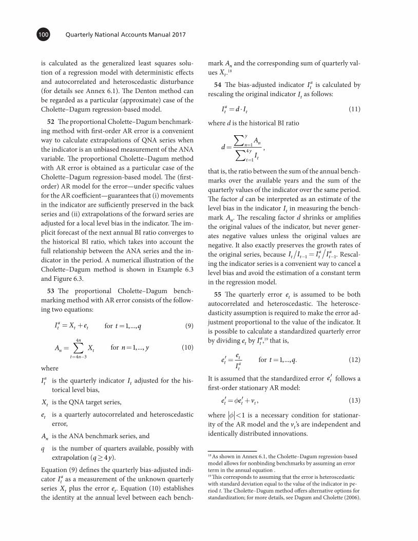
is calculated as the generalized least squares solu-tion of a regression model with deterministic effects and autocorrelated and heteroscedastic disturbance (for details see Annex 6.1). The Denton method can be regarded as a particular (approximate) case of the Cholette–Dagum regression-based model.
52 The proportional Cholette–Dagum benchmark-ing method with first-order AR error is a convenient way to calculate extrapolations of QNA series when the indicator is an unbiased measurement of the ANA variable. The proportional Cholette–Dagum method with AR error is obtained as a particular case of the Cholette–Dagum regression-based model. The (first-order) AR model for the error—under specific values for the AR coefficient—guarantees that (i) movements in the indicator are sufficiently preserved in the back series and (ii) extrapolations of the forward series are adjusted for a local level bias in the indicator. The im-plicit forecast of the next annual BI ratio converges to the historical BI ratio, which takes into account the full relationship between the ANA series and the in-dicator in the period. A numerical illustration of the Cholette–Dagum method is shown in Example 6.3 and Figure 6.3.
53 The proportional Cholette–Dagum bench-marking method with AR error consists of the follow-ing two equations:
I X eta
t t= + for t q=1,..., (9)
A Xn tt n
n
== −∑
4 3
4
for n y=1,..., (10)
where
Ita is the quarterly indicator It adjusted for the his-
torical level bias,
Xt is the QNA target series,
et is a quarterly autocorrelated and heteroscedastic error,
An is the ANA benchmark series, and
q is the number of quarters available, possibly with extrapolation (q y≥ 4 ).
Equation (9) defines the quarterly bias-adjusted indi-cator It
a as a measurement of the unknown quarterly series Xt plus the error et. Equation (10) establishes the identity at the annual level between each bench-
mark An and the corresponding sum of quarterly val-ues Xt .18
54 The bias-adjusted indicator Ita is calculated by
rescaling the original indicator It as follows:
I d Ita
t= ⋅ (11)
where d is the historical BI ratio
dA
I
nn
y
tt
y= =
=
∑∑
1
1
4 ,
that is, the ratio between the sum of the annual bench-marks over the available years and the sum of the quarterly values of the indicator over the same period. The factor d can be interpreted as an estimate of the level bias in the indicator It in measuring the bench-mark An. The rescaling factor d shrinks or amplifies the original values of the indicator, but never gener-ates negative values unless the original values are negative. It also exactly preserves the growth rates of the original series, because I I I It t t
ata
− −=1 1. Rescal-ing the indicator series is a convenient way to cancel a level bias and avoid the estimation of a constant term in the regression model.
55 The quarterly error et is assumed to be both autocorrelated and heteroscedastic. The heterosce-dasticity assumption is required to make the error ad-justment proportional to the value of the indicator. It is possible to calculate a standardized quarterly error by dividing et by It
a,19 that is,
′ =eeIt
t
ta for t q=1,..., . (12)
It is assumed that the standardized error ′et follows a first-order stationary AR model:
′ = ′ +e e vt t tφ , (13)
where φ <1 is a necessary condition for stationar-ity of the AR model and the vt’s are independent and identically distributed innovations.
18 As shown in Annex 6.1, the Cholette–Dagum regression-based model allows for nonbinding benchmarks by assuming an error term in the annual equation .19 This corresponds to assuming that the error is heteroscedastic with standard deviation equal to the value of the indicator in pe-riod t. The Cholette–Dagum method offers alternative options for standardization; for more details, see Dagum and Cholette (2006).
6240-082-FullBook.indb 100 10/18/2017 6:09:10 PM

Benchmarking and Reconciliation 101
Example 6.3 The Proportional Cholette–Dagum Method with Autoregressive Error
Indicator Proportional Cholette–Dagum MethodEstimated Quarterly BI Ratios Indicator
Bias-adjusted Indicator
Quarter-to- Quarter Rate of Change
(%)
Year-on- Year
Rate of Change
(%)
Annual Data
Annual BI Ratio
Benchmarked Data (Ø = 0.8)
Quarter-to- Quarter Rate of Change
(%)
Year-on- Year
Rate of Change
(%) (1) (2) (3)(4)=(3)/
(1)(5) (6)
q1 2010 99.4 249.2 247.7 2.4917
q2 2010 99.6 249.7 0.2 248.4 0.3 2.4940
q3 2010 100.1 250.9 0.5 250.4 0.8 2.5010
q4 2010 100.9 252.9 0.8 253.6 1.3 2.5131
2010 400.0 1,000.0 2.5000 1,000.0
q1 2011 101.7 255.0 0.8 2.3 257.4 1.5 3.9 2.5307
q2 2011 102.2 256.2 0.5 2.6 259.4 0.8 4.4 2.5386
q3 2011 102.9 258.0 0.7 2.8 261.0 0.6 4.3 2.5368
q4 2011 103.8 260.2 0.9 2.9 262.1 0.4 3.4 2.5255
2011 410.6 2.7 1,040.0 2.5329 1,040.0 4.0
q1 2012 104.9 263.0 1.1 3.1 262.7 0.2 2.1 2.5040
q2 2012 106.3 266.5 1.3 4.0 264.6 0.7 2.0 2.4894
q3 2012 107.3 269.0 0.9 4.3 266.2 0.6 2.0 2.4812
q4 2012 107.8 270.2 0.5 3.9 267.3 0.4 2.0 2.4794
2012 426.3 3.8 1,060.8 2.4884 1,060.8 2.0
q1 2013 107.9 270.5 0.1 2.9 268.0 0.3 2.0 2.4838
q2 2013 107.5 269.5 −0.4 1.1 267.4 −0.2 1.1 2.4875
q3 2013 107.2 268.7 −0.3 −0.1 267.0 −0.2 0.3 2.4906
q4 2013 107.5 269.5 0.3 −0.3 268.0 0.4 0.3 2.4932
2013 430.1 0.9 — — 1,070.4 0.9
Historical BI Ratio and Bias-Adjusted IndicatorThe historical BI ratio (2.5069) is calculated as the ratio of the sum of the annual data from 2010 to 2012 (3,100.8) to the sum of the quarterly values of the indicator from q1 2010 to q4 2012 (1,236.9). The historical BI ratio is shown as a dotted horizontal line in the bottom panel of Figure 6.3. It represents the long-term average of the annual BI ratio. The bias-adjusted indicator in column 2 is obtained by multiplying the indicator series by the historical BI ratio (2.5069).
Extrapolation with AR Error In this example, we use the value 0.84 for the AR parameter. The error for q4 2012 is equal to 2.9709 (i.e., 270.2452 − 267.2743). Using formulas , , and , quarterly extrapolations for 2013 are derived as the sum of the bias-adjusted indicator in the four quarters of 2013 and AR extrapolation of the last quarterly error in q4 2012:
q1 2013 270.5 – [(0.84) × 2.9709] = 270.5 − 2.4956 = 268.0
q2 2013 269.5 – [(0.842) × 2.9709] = 269.5 − 2.0963 = 267.4
q3 2013 268.7 – [(0.843) × 2.9709] = 268.7 − 1.7609 = 267.0
q4 2013 269.5 – [(0.844) × 2.9709] = 269.5 − 1.4791 = 268.0
The extrapolated quarterly BI ratio for q4 2013 (2.4932) is the midpoint between the quarterly BI ratio for q4 2012 (2.4794) and the historical BI ratio (2.5069). In fact, as explained in the text, a value of 0.84 for Ø eliminates 50 percent of the bias after one year from the last available quar-ter. It is worth noting that for 2013 (i) the annual growth rate of the QNA extrapolated series is 0.9 percent (the Denton method extrapolates a 0.4% increase in 2013) and (ii) the quarterly extrapolated growth rates of the QNA series are different from the quarterly growth rates shown by the indicator.
(These results are illustrated in Figure 6.3. Rounding errors in the table may occur.)
6240-082-FullBook.indb 101 10/18/2017 6:09:10 PM

Quarterly National Accounts Manual 2017102
Figure 6.3 Solution to the Extrapolation Problem: The Proportional Cholette–Dagum Method with Autoregressive Error
The Indicator and the Derived Benchmarked Series
Benchmark-to-Indicator Ratio
245.0
250.0
255.0
260.0
265.0
270.0
98.0
100.0
102.0
104.0
106.0
108.0
2010 2011 2012 2013
(The corresponding data are given in Example 6.3)
Indicator (left-hand axis)Benchmarked Data with Proportional Denton Method (right-hand axis)Benchmarked Data with Proportional Cholette-Dagum Method with Autoregressive Error (right-hand axis)
Back Series Forward Series
2.46
2.48
2.50
2.52
2.54
2.56
2010 2011 2012 2013Proportional Denton MethodProportional Cholette-Dagum Method with Autoregressive ErrorHistorical BI Ratio
6240-082-FullBook.indb 102 10/18/2017 6:09:10 PM

Benchmarking and Reconciliation 103
56 The AR model assumption for the standardized error ′et implies that the quarterly BI ratio is also dis-tributed according to a first-order AR model. In fact, the standardized error ′et is proportional to the quar-terly BI ratio. This is easily shown by rearranging the elements of equations (9) and (12)
X I e
X I e I
eI X
I
t ta
t
t ta
t ta
tta
t
ta
= −
= − ′
′ =−
(14)
which corresponds to the term (with opposite sign) that defines the proportional criterion minimized by the Denton method. It can be shown that as the value of φ in model (13) approaches 1, the bench-marked series obtained with the proportional Cho-lette–Dagum method converges to the solution given by the proportional Denton method.
57 In extrapolation, the quarterly (standardized) error is calculated by multiplying the AR parameter recursively by the last quarterly error observed:
′ = ′+e ey kk
yˆ4 4φ for any k>0. (15)
When φ lies between 0 and 1, the extrapolated error ′ +e y kˆ4 tends to zero as k increases (at different rates
depending on the value of φ). As ′ →+e y k4 0 (and so does e y k4 + ), the extrapolated QNA variable converges to the bias-adjusted indicator:
X I d Iy k y ka
y kˆ
4 4 4+ + +→ = ⋅ .
The previous expression is equivalent to say that the extrapolated BI ratio converges to the historical BI ratio:
XI
dA
I
y k
y k
nn
y
tt
y4
4
1
1
4+
+
=
=
→ =∑∑
.
58 The value of the AR parameter φ determines how fast the QNA extrapolated series converges to the bias-adjusted indicator. Values of φ closer to zero tend to eliminate quickly the bias and provide fast conver-gence rates to I y k
a4 + ; on the contrary, values closer to
1 would maintain the bias in extrapolated quarters. However, a value of φ too far from 1 would generate a QNA series with growth rates distant from those of
the indicator (both in the back series and in the for-ward series). An optimal value of φ should balance the trade-off between adjusting extrapolations for the current bias and maintaining close adherence to the growth rates of the indicator.20
59 A convenient value for the AR parameterφ in model (13) is 0.84. This particular value ensures that (about) 50 percent of the bias observed in the last quarterly error is eliminated after one year. In fact, using formula (15) with φ= 0 84. and k= 4 returns
e′ = ′ ≈ ′+˘ ( . ) .e e ey y y4 44
4 40 84 0 5 .
A 50 percent reduction in the bias implies that the quarterly BI ratio in the fourth quarter of the next year is the midpoint between the last observed quar-terly BI ratio and the historical BI ratio d. Although not grounded on strong theoretical arguments, this solution appears pragmatic and suitable to many practical benchmarking problems. However, different values may be chosen according to the development of the annual BI ratio in the most recent years:
• When the annual BI ratio is erratic, it is best to eliminate rapidly the bias. In such situations, the value ofφ should be selected in a range between 0.71 and 0.84. The minimum value 0.71 leads to a 75 percent reduction of the bias after one year.
• When the annual BI ratio shows persistent movements, it may be convenient to maintain (part of) the bias in extrapolation. A value ofφbetween 0.84 and 0.93 would serve this purpose. The maximum value 0.93 yields a 25 percent re-duction of the bias after one year.
60 To sum up, the proportional Cholette–Dagum method with AR error method leads, on average, to more accurate extrapolation (and smaller revisions) than the Denton method when the indicator is an un-biased measurement of the ANA variable. Using the Cholette–Dagum solution, a local bias in the indica-tor arising in the most recent years can be adjusted through an AR convergence process from the last cal-culated quarterly error toward the historical BI ratio.
20 For quarterly series, Dagum and Cholette (2006) suggest a range of values ofφ between 0.343 and 0.729 (temporally consistent with the range [0.7; 0.9] suggested for monthly series). However, this range could lead to sizable differences between the short-term dynamics of the QNA series and the indicator.
6240-082-FullBook.indb 103 10/18/2017 6:09:12 PM

Quarterly National Accounts Manual 2017104
The Cholette–Dagum method provides an automatic solution to overcome the shortcomings of the Denton method in extrapolation. Clearly, the relative perfor-mance of the Cholette–Dagum and Denton methods should be assessed on a continuous basis by com-paring their QNA extrapolations with the new ANA benchmarks.
61 Ultimately, the choice between the Denton method (with or without adjustment for extrapola-tion) and Cholette–Dagum method could be a sub-jective call. Compilers may decide to use either of the two methods based on the properties of each bench-marking problem in the QNA. For the same variable, however, a definite choice between the two methods should be done. The same method should be used for calculating both the back series and forward se-ries of ANA variables. Once a method is chosen for a variable, the method should be used consistently over time. Switching between Denton and Cholette–Dagum methods for the same variable may cause re-visions that are difficult to explain. If a change in the method is warranted, it should be done at a time of a major revision of national accounts. The use of bench-marking methods in the QNA should be documented clearly in the metadata.
62 It is worth noting here that the regression-based temporal disaggregation method proposed by Chow and Lin (1971) and its variants21 can also be considered particular cases of the Cholette–Dagum regression-based framework. The Chow–Lin method is used by some countries for the compilation of the QNA. Simi-lar to the Cholette–Dagum solution described in this section, the Chow–Lin method assumes a first-order AR model to distribute smoothly the quarterly error and preserve as much as possible the movements of the indicator. However, this method requires that re-gression parameters are estimated from the data. Bad estimation of the parameters may lead to inaccurate QNA results, therefore a more careful investigation of the benchmarking results is required when using the Chow–Lin approach.22
63 When the Chow–Lin method is chosen, com-pilers should be aware that this approach requires expertise and statistical background to validate the results of the estimation process. Estimated param-
21 See Fernández (1981) and Litterman (1983). 22 Further details on the Chow–Lin method are given in Annex 6.1.
eters of the regression model should be validated using standard diagnostics (residual tests, correla-tion, etc.). The value of regression coefficient for the related indicator should be positive and statistically different from zero. Only one indicator should be used in the regression model, with a possible con-stant term to adjust for the different levels of the variables. Finally, the estimated value for the AR coefficient should be positive and sufficiently close to one to preserve the short-term dynamics of the indicator.
Specific IssuesFixed Coefficient Assumptions
64 The benchmarking methodology can be used to avoid potential step problems in different areas of national accounts compilation. One important example is the frequent use of assumptions of fixed coefficients relating inputs (total or part of interme-diate consumption or inputs of labor and capital) to output: input–output (IO) ratios. IO ratios or similar coefficients may be derived from annual supply and use tables, production surveys, or other internal in-formation available. Fixed IO ratios can be consid-ered a benchmark–indicator relationship, where the available series (usually output) is the indicator for the missing one (usually intermediate consumption) and the IO ratio (or its inverse) is the BI ratio. If IO ratios are changing from year to year but are kept constant within each year, a step problem is created. Accord-ingly, the Denton technique can be used to generate smooth time series of quarterly IO ratios based on annual (or less frequent) IO coefficients. The missing variable can be reconstructed by multiplying (or di-viding) the quarterly IO ratios (derived by the Denton technique) by the available series. For instance, the derived quarterly IO ratios multiplied by quarterly output will provide an implicit estimate of quarterly intermediate consumption. Systematic trends can be identified to forecast IO ratios for the most recent quarters. Alternatively, the Cholette–Dagum method can be used to improve extrapolations of IO ratios based on historical behavior.
Seasonal Effects
65 It is possible to assign specific seasonal varia-tions to a QNA variable when applying benchmark-ing. This solution may be needed when the true
6240-082-FullBook.indb 104 10/18/2017 6:09:12 PM

Benchmarking and Reconciliation 105
underlying seasonal pattern in the QNA variable is not fully represented by the indicator. For example, an indicator may be available only in seasonally adjusted form, whereas the QNA variable is known to have a seasonal component. Specific seasonal effects may also be assumed in the distribution of annual coef-ficients, when the coefficients are subject to seasonal variations within the year. IO ratios may vary cycli-cally owing to inputs that do not vary proportionally with output, typically fixed costs such as labor, capital, or overhead (e.g., heating and cooling). Similarly, the ratio between income flows (e.g., dividends) and their related indicators (e.g., profits) may vary between quarters.
66 To incorporate a known seasonal pattern in the target QNA variable, without introducing steps in the series, the following multistep solution should be adopted:
1. Seasonally adjust the quarterly indicator. This step is needed to remove any unwanted sea-sonal effects in the indicator (if any) from the QNA series. Seasonal adjustment procedures should be applied using the guidelines pro-vided in Chapter 7. Misguided attempts to correct the problem in the original data could distort the underlying trends. This step is not required if the indicator is already seasonally adjusted.
2. Multiply the seasonally adjusted indicator se-ries by the known seasonal factors. The sea-sonal pattern can be fixed or variable over the years. It is convenient to impose quarterly sea-sonal factors that average to 1 in each year,23 so that the underlying trend of the original indicator is not changed. Seasonal factors can also be extracted from another series through a seasonal adjustment procedure, when the seasonal behavior of that particular series is deemed to approximate the seasonality in the QNA variable.
3. Benchmark the quarterly series with superim-posed seasonal effects derived at step 2 to the ANA target variable.
23 As an example, quarterly seasonal coefficients that average to 1 are [0.97, 1.01, 0.99, 1.03]. This pattern would assume lower-than-average activity in the first (q1) and third (q3) quarters and higher-than-average activity in the second (q2) and fourth (q4) quarters.
Dealing with Difficult Benchmarking ProblemsShort Series
67 For the back series, the Denton and Cholette–Dagum methods require a minimum of two years in the ANA variable and eight quarters in the indicator series. The results obtained with two years are in line with the stated objectives of benchmarking. For the forward series, however, two years of data may not be enough to appreciate the extrapolation accuracy of the methods. A longer period is needed to moni-tor the movements in the BI ratio, in order to identify possible divergence between the movements in the indicator and those in the ANA variable. When the Denton or Cholette–Dagum methods are used for ex-trapolation, a minimum of five years in both the ANA variable and the indicator series is recommended.
Series with Breaks
68 Benchmarking can produce inaccurate results when an annual variable contains a structural break in one year and the corresponding indicator does not include the same break (and vice versa).24 The quar-terly benchmarked series could indicate an incorrect timing of the start of the break and affect adjacent quarters that are not supposed to be affected. These situations typically happen when the ANA variable and the quarterly indicator have different coverage. For example, the national accounts data may include informal activities of a specific industry, while the quarterly indicator may only cover formal ones. If a break occurs in the informal sector only, the indicator will not show any change.
69 The first step to tackle this problem is to under-stand the nature of the break and verify the underlying reasons why the break does not show up consistently in the two measurements. When the break is in the ANA variable but not in the indicator, the quarterly indi-cator should be adjusted to match the corresponding shift in the ANA variable. The best possible measure-ment of the timing of the break should be done in the quarterly pattern of the adjusted indicator. When the break is in the indicator and not in the ANA variable, compilers should investigate whether the indicator is
24 In this context, a structural break is defined as a sizeable (up-ward or downward) change in the level of a variable. The break can be either permanent or transitory.
6240-082-FullBook.indb 105 10/18/2017 6:09:12 PM
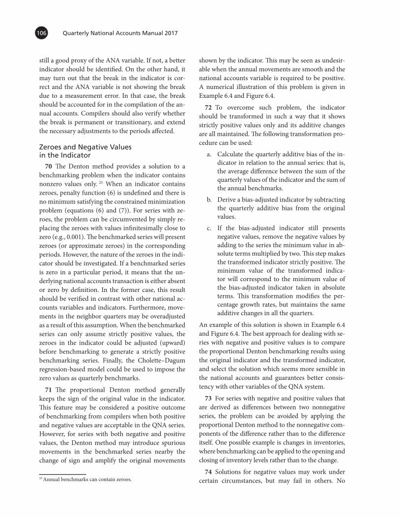
Quarterly National Accounts Manual 2017106
still a good proxy of the ANA variable. If not, a better indicator should be identified. On the other hand, it may turn out that the break in the indicator is cor-rect and the ANA variable is not showing the break due to a measurement error. In that case, the break should be accounted for in the compilation of the an-nual accounts. Compilers should also verify whether the break is permanent or transitionary, and extend the necessary adjustments to the periods affected.
Zeroes and Negative Values in the Indicator
70 The Denton method provides a solution to a benchmarking problem when the indicator contains nonzero values only. 25 When an indicator contains zeroes, penalty function (6) is undefined and there is no minimum satisfying the constrained minimization problem (equations (6) and (7)). For series with ze-roes, the problem can be circumvented by simply re-placing the zeroes with values infinitesimally close to zero (e.g., 0.001). The benchmarked series will present zeroes (or approximate zeroes) in the corresponding periods. However, the nature of the zeroes in the indi-cator should be investigated. If a benchmarked series is zero in a particular period, it means that the un-derlying national accounts transaction is either absent or zero by definition. In the former case, this result should be verified in contrast with other national ac-counts variables and indicators. Furthermore, move-ments in the neighbor quarters may be overadjusted as a result of this assumption. When the benchmarked series can only assume strictly positive values, the zeroes in the indicator could be adjusted (upward) before benchmarking to generate a strictly positive benchmarking series. Finally, the Cholette–Dagum regression-based model could be used to impose the zero values as quarterly benchmarks.
71 The proportional Denton method generally keeps the sign of the original value in the indicator. This feature may be considered a positive outcome of benchmarking from compilers when both positive and negative values are acceptable in the QNA series. However, for series with both negative and positive values, the Denton method may introduce spurious movements in the benchmarked series nearby the change of sign and amplify the original movements
25 Annual benchmarks can contain zeroes.
shown by the indicator. This may be seen as undesir-able when the annual movements are smooth and the national accounts variable is required to be positive. A numerical illustration of this problem is given in Example 6.4 and Figure 6.4.
72 To overcome such problem, the indicator should be transformed in such a way that it shows strictly positive values only and its additive changes are all maintained. The following transformation pro-cedure can be used:
a. Calculate the quarterly additive bias of the in-dicator in relation to the annual series: that is, the average difference between the sum of the quarterly values of the indicator and the sum of the annual benchmarks.
b. Derive a bias-adjusted indicator by subtracting the quarterly additive bias from the original values.
c. If the bias-adjusted indicator still presents negative values, remove the negative values by adding to the series the minimum value in ab-solute terms multiplied by two. This step makes the transformed indicator strictly positive. The minimum value of the transformed indica-tor will correspond to the minimum value of the bias-adjusted indicator taken in absolute terms. This transformation modifies the per-centage growth rates, but maintains the same additive changes in all the quarters.
An example of this solution is shown in Example 6.4 and Figure 6.4. The best approach for dealing with se-ries with negative and positive values is to compare the proportional Denton benchmarking results using the original indicator and the transformed indicator, and select the solution which seems more sensible in the national accounts and guarantees better consis-tency with other variables of the QNA system.
73 For series with negative and positive values that are derived as differences between two nonnegative series, the problem can be avoided by applying the proportional Denton method to the nonnegative com-ponents of the difference rather than to the difference itself. One possible example is changes in inventories, where benchmarking can be applied to the opening and closing of inventory levels rather than to the change.
74 Solutions for negative values may work under certain circumstances, but may fail in others. No
6240-082-FullBook.indb 106 10/18/2017 6:09:12 PM

Benchmarking and Reconciliation 107
Example 6.4 Benchmarking Series with Positive and Negative Values: Use of Strictly Positive Indicators
Indicator Proportional Denton Method Transformed IndicatorProportional Denton Method using
the Transformed Indicator
Level
Quarter-to- Quarter Rate of Change
Benchmarked Series
Quarter-to- Quarter Rate
of ChangeLevel
Quarter-to- Quarter Rate of Change
Benchmarked Series
Quarter-to- Quarter Rate of
Change
q1 2010 20.0 107.8 94.6 67.8
q2 2010 15.0 −25.0 64.5 −40.2 89.6 −5.3 63.6 −6.3
q3 2010 10.0 −33.3 23.9 −62.9 84.6 −5.6 58.8 7.5
q4 2010 −60.0 −700.0 3.7 −84.5 14.6 −82.8 9.8 −83.3
2010 −15.0 200.0 283.3 200.0
q1 2011 10.0 −116.7 7.6 104.4 84.6 480.0 55.1 460.8
q2 2011 20.0 100.0 29.8 294.5 94.6 11.8 61.2 11.0
q3 2011 45.0 125.0 92.8 211.1 119.6 26.4 79.0 29.2
q4 2011 75.0 66.7 169.8 82.8 149.6 25.1 104.7 32.4
2011 150.0 300.0 448.3 300.0
q1 2012 90.0 20.0 166.1 −2.1 164.6 10.0 126.6 21.0
q2 2012 100.0 11.1 151.8 −8.6 174.6 6.1 143.7 13.5
q3 2012 110.0 10.0 141.8 −6.6 184.6 5.7 158.7 10.4
q4 2012 120.0 9.1 140.3 −1.0 194.6 5.4 171.0 7.7
2012 420.0 600.0 718.3 600.0
Negative Values in the Indicator and Growth RatesIn column 1, the indicator presents a negative value in q4 2010 (−60). The growth rate for q1 2011 [10–(–60)]/–60 = –1.167 ⇒ – 116.7% is misleading because it would signal negative growth while the series increases from −60 to 10.
Derive a Bias-Adjusted, Strictly Positive Indicator The following procedure produces a bias-adjusted indicator with strictly positive values:
1. Calculate the quarterly additive bias of the indicator in relation to the annual series, that is, the average difference between the sum of the quarterly values of the indicator and the sum of the annual benchmarks:
Sum of quarterly values: 20 + 15 + 10 − 60 + … + 120 = 555 Sum of annual benchmarks: 200 + 300 + 600 = 1,100 Quarterly additive bias: (555 − 1,100)/12 = −45.4.
2. Derive a bias-adjusted indicator by subtracting the quarterly additive bias from the original values:
q1 2010: 20 – (−45.4) = 65.4 q2 2010: 15 – (−45.4) = 60.4 q3 2010: 10 – (−45.4) = 55.4 q4 2010: –60 – (−45.4) = −14.6, and so forth.
3. If the bias-adjusted indicator still contains negative values, transform the series by adding the minimum value in absolute terms multi-plied by two, that is,
q1 2010: 65.4 + (2 × 14.6) = 94.6 q2 2010: 60.4 + (2 × 14.6) = 89.6 q3 2010: 55.4 + (2 × 14.6) = 84.6 q4 2010: −14.6 + (2 × 14.6) = 14.6, and so forth.
The minimum value in the transformed indicator (column 3) is the minimum value of the bias-adjusted indicator taken in absolute terms (14.6 in q4 2010). Note that the transformation modifies the growth rates, but the additive changes of the transformed indicator are equal to those of the original indicator in all quarters.
Annual Benchmarks with Strictly Positive Values In this example, the annual benchmarks are positive and all distant from zero (200 in 2010, 300 in 2011, and 600 in 2012). It is reasonable to assume that the quarterly values are also strictly positive. Applying the proportional Denton method with the original indicator (column 2) would force the quarterly benchmarked series to preserve the negative value in q4 2010 (−79.2). Conversely, the proportional Denton method with the bias-adjusted, strictly positive indicators (column 4) produces a benchmarked series that correctly reproduce the additive changes and returns all positive values (9.8 in q4 2010).
(These results are illustrated in Figure 6.4. Rounding errors in the table may occur.)
6240-082-FullBook.indb 107 10/18/2017 6:09:12 PM

Quarterly National Accounts Manual 2017108
Figure 6.4 Solution to Positive and Negative Values: Use of Strictly Positive Indicators
The Indicator and the Derived Benchmarked Series(The corresponding data are given in Example 6.4)
-100.0
-50.0
0.0
50.0
100.0
150.0
200.0
2010 2011 2012
Indicator Benchmarked Data with Proportional Denton Method with Original Indicator Benchmarked Data with Proportional Denton Method with Strictly Positive Indicator
Back Series Forward Series
matter how good the method is, a new combination of negative and positive values may appear in the data that can create discontinuity in the series. Bench-marking problems with negative and positive values should always be treated with care.
Benchmarking Without a Related Indicator
75 Quarterly values may have to be derived by using mathematical techniques that distribute the an-nual values into quarters without using a related quar-terly indicator. These techniques should be avoided as much as possible in the compilation of QNA series because they do not reflect the true movements in the economy. These situations should be prevented when the QNA system is put in place by defining an ap-propriate level of detail of the ANA variables, taking into account the quarterly sources available from data providers. Benchmarking without a related indicator is acceptable only for series that move smoothly from one quarter to the next. Moreover, the size of the vari-able should be contained in order to reduce its impact
on the levels of GDP and other main aggregates. A possible example of a stable series is consumption of fixed capital (when capital formation is fairly stable). In such cases, the ANA series should be interpolated in a way such that the quarterly values provide move-ments that are as stable as possible. This approach minimizes the impact of these items on the dynamics arising from the rest of the accounts.
76 The optimal method is provided by the inter-polation technique suggested by Boot, Feibes and Lisman (1967). The Boot–Feibes–Lisman method looks for the quarterly values that minimize the sum of squares of the difference between successive quarters:
minX t t
t
y
t
X X− −=∑ 1
2
2
4
(16)
subject to the annual constraints
X A n yt nt n
n
= == −∑
4 3
4
1for , ..., .
6240-082-FullBook.indb 108 10/18/2017 6:09:13 PM

Benchmarking and Reconciliation 109
77 Conveniently, the Boot–Feibes–Lisman solu-tion can be derived by applying the proportional Denton method with a constant indicator. If we as-sume I Ct = , penalty function (6) becomes
min min ,X
t t
t
y
X t tt
y
t t
XC
XC C
X X−
⇔ −
−
=−
=∑ ∑1
2
2
4
2 12
2
41
which corresponds to the penalty function mini-mized by the Boot–Feibes–Lisman shown in equation (16) multiplied by a constant factor (which does not change the solution of the minimization problem). When extrapolations are needed, the quarterly vari-able can be extrapolated based on time-series models (see Chapter 10). Alternatively, an annual forecast of the next benchmark could be included in the bench-marking process. In both cases, because the variable is expected to be highly predictable, revisions to QNA variables would be very limited in future releases.
Benchmarking and Compilation Procedures
78 Benchmarking should be an integral part of the compilation process and should be conducted at the most detailed compilation level. In practice, this may imply benchmarking different series in stages, where data for some series—which have already been benchmarked—are used to estimate other series, fol-lowed by a second or third round of benchmarking. The actual arrangements will vary depending on the particularities of each case.
79 As an illustration, annual data may be avail-able for all products, but quarterly data are available only for the main products. If it is decided to use the sum of the quarterly data as an indicator for the other products, the ideal procedure would be first to benchmark each of the products for which quarterly data are available to the annual data for that prod-uct, and then to benchmark the quarterly sum of the benchmarked estimates for the main products to the total. Of course, if all products were moving in simi-lar ways, this would give similar results to directly benchmarking the quarterly total to the annual total.
80 In other cases, a second or third round of bench-marking may be avoided and compilation procedure simplified. For instance, a current price indicator can be constructed as the product of a quantity indicator and a price indicator without first benchmarking the quantity and price indicators to any corresponding
annual benchmarks. Similarly, a volume indicator can be constructed as a current price indicator divided by a price indicator without first benchmarking the cur-rent price indicator. Also, if output at constant prices is used as an indicator for intermediate consumption, the (unbenchmarked) constant price output indicator can be benchmarked to the annual intermediate con-sumption data directly. It can be shown that the result is identical to first benchmarking the output indicator to annual output data, and then benchmarking the re-sulting benchmarked output estimates to the annual intermediate consumption data.
81 To derive quarterly constant price data by deflat-ing current price data, the correct procedure would be first to benchmark the quarterly current price in-dicator and then to deflate the benchmarked quarterly current price data. If the same price indices are used in the annual and quarterly accounts, the sum of the four quarters of constant price data should be taken as the annual estimate, and a second round of bench-marking is unnecessary. As explained in Chapter 8, annual deflators constructed as unweighted averages of monthly or quarterly price data can introduce an aggregation over time error in the annual deflators and subsequently in the annual constant price data that can be significant if there is quarterly volatility. Moreover, if, in those cases, quarterly constant price data are de-rived by benchmarking a quarterly constant price in-dicator derived by deflating the current price indicator to the annual constant price data, the aggregation over time error will be passed on to the implicit quarterly deflator, which will differ from the original price in-dices. Thus, in those cases, annual constant price data should in principle be derived as the sum of quarterly or even monthly deflated data if possible. If quarterly volatility is insignificant, however, annual constant price estimates can be derived by deflating directly and then benchmarking the quarterly constant price estimates to the annual constant price estimates.
82 Finally, benchmarking can be performed before or after seasonal adjustment. When benchmarking is applied on the unadjusted data only, seasonal adjust-ment is performed on the results of benchmarking (i.e., the benchmarked series). On the other hand, sea-sonal adjustment can be done prior to benchmarking when the seasonal adjustment method is applied to the short-term indicators (monthly or quarterly). In this case, the seasonally adjusted indicator should be
6240-082-FullBook.indb 109 10/18/2017 6:09:13 PM

Quarterly National Accounts Manual 2017110
benchmarked to the annual accounts. Chapter 7 dis-cusses in more details about benchmarking of season-ally adjusted data.
Benchmarking and Revisions
83 To avoid introducing distortions in the series, incorporation of new annual data for one year will generally require revision of previously published quarterly data for several years. Benchmarking meth-ods with movement preservation (like the Denton method and the Cholette–Dagum method) minimize the impact of revisions on the historical movements of the QNA series. In principle, previously published QNA estimates for all preceding and following years may have to be adjusted to maximally preserve the short-term movements in the indicator, if the errors in the indicator are large. In practice, however, with most benchmarking methods, the impact of new an-nual data will gradually be diminishing and zero for sufficiently distant periods.
84 Ideally, revisions to quarterly indicators should be incorporated in the QNA series as soon as possible to reflect the most up-to-date short-term information available. This is particularly relevant for the forward series, which should immediately incorporate revisions to preliminary values of the indicators for the previous quarters on the basis of more up-to-date and comprehensive source data. If revisions to preliminary information in the current year are disregarded, the QNA may easily lead to bi-ased extrapolations for the next years. For the back series, revisions to previous years of the indicator should be reflected in the QNA series at the time when revisions to new or revised ANA benchmarks are incorporated.
85 Revisions to some previously published QNA estimates can be avoided by freezing the quarterly values for those periods. This practice should be defined clearly in the revision policy of QNA data and not be changed from one quarter to the next without advance communication to users. To avoid introducing significant distortions to the bench-marked series, however, at least two to three years preceding (and following) years should be allowed to be revised each time new annual data become available. In general, the impact on more distant years will be negligible.
Reconciliation of QNA Series86 The benchmarking methods discussed in this
chapter adjust one indicator at a time to generate quarterly values in line with corresponding ANA benchmarks. The benchmarking adjustment pro-cess is applied individually to each variable and does not take into account any accounting relation-ship between the QNA series. Consequently, the benchmarked quarterly series may not automati-cally form a consistent set of accounts. For example, the independently derived quarterly estimates of GDP from the production side may differ from the independently derived quarterly estimates of GDP from the expenditure side, even though the annual data are consistent. Another example is when quar-terly totals derived from estimates by institutional sector differ from the same quarterly totals derived from estimates by economic activity. Finally, quar-terly discrepancies may arise when seasonal adjust-ment is applied directly to both QNA components and aggregates (see Chapter 7 for more details on the direct versus indirect seasonally adjusted approaches).
87 Quarterly inconsistencies between QNA se-ries should be addressed and resolved at the vari-ous stages of QNA compilation. Discrepancies can be minimized by using coherent (when not equal) quarterly indicators for production, expenditure, and income flows pertaining to the same industry or product. Large discrepancies indicate that there are large inconsistencies between the short-term movements of interconnected QNA series. Some discrepancies in the accounts can also be elimi-nated in the compilation stage by benchmarking (or seasonally adjusting) different parts of the accounts at the most detailed level and building aggregates from the benchmarked (or seasonally adjusted) components. The discrepancies that remain after this careful investigation process should be eliminated using automatic adjustment procedures.
88 This section presents statistical methods to transform a set of quarterly indicators into a consistent system of QNA series that satisfy both annual con-straints and quarterly constraints. These methods are called reconciliation methods. The annual constraints are those from the ANA system and correspond to the
6240-082-FullBook.indb 110 10/18/2017 6:09:13 PM

Benchmarking and Reconciliation 111
same ANA totals considered for benchmarking. The quarterly constraints are linear, contemporaneous aggregations26 of the QNA series. These can be of two different types:27
· Endogenous constraints. In the national ac-counts there are endogenous accounting re-strictions that should be met by the variables at any frequency: for example, the sum of gross output and imports of a product should be equal to the sum of final and intermediate uses of that product (net of valuation and adjust-ment items) or the difference of gross output and intermediate consumption is equal to gross value added. These identities can be added as quarterly accounting restrictions between the variables involved in the constrained minimi-zation problem.
· Exogenous constraints. These are usually QNA aggregates that are independently derived from the system under adjustment. For example, quarterly estimates of value added by institu-tional sectors can be adjusted so that their sum is equal to quarterly gross value added for the total economy derived by economic activity. It has to be noted that exogenous constraints must satisfy the set of annual constraints. In the exam-ple above, the annual total gross value added by industry must be equal to the annual total gross value added by institutional sector. A numeri-cal illustration of a three-variable QNA system with an independently derived quarterly sum is shown in Example 6.5.
89 In the QNA, the main objectives of reconcilia-tion are as follows:
· to provide quarterly data that are (i) temporally consistent with the ANA data that is such that the sum (or the average) of the quarterly data is equal to the annual benchmark and, at the same time, (ii) consistent with (endogenous and exogenous)
26 Contemporaneous means that the quarterly constraints refer to the current quarter only (no lead or lagged relationships). It is also assumed that these quarterly relationships are linear combination of the variables. Nonlinear restrictions between the variables may also be useful in the adjustment process (e.g., be-tween price and volume measures, or unadjusted and seasonally adjusted series), but they are not dealt with in this presentation for the sake of simplicity. 27 This manual considers only quarterly binding constraints. Quarterly constraints are nonbinding when they are subject to changes in the reconciliation process.
quarterly constraints that is such that linear com-binations of the quarterly adjusted data are equal to given values available in every observed quar-ter; and
· to preserve as much as possible the quarterly movements in the indicator under the restric-tions provided by the ANA data and the quar-terly aggregation constraints.
90 Differently from benchmarking, reconciliation methods have to satisfy quarterly constraints in ex-trapolation. The forward series return quarterly val-ues that are consistent with the quarterly extrapolated constraints. When there are exogenous constraints, they should always include estimates for the extrapo-lated quarters (either derived with the enhanced Den-ton method or the Cholette–Dagum method with AR error). The variables of the system will be extrapo-lated in accord with the quarterly extrapolated con-straints. When there are endogenous constraints only, the individual variables of the system should be first extrapolated using the preferred univariate method for extrapolation. The extrapolated QNA variables can then be used as input series of the reconciliation methods.
91 Given the stated objectives of reconciliation, the multivariate proportional Denton method is the best solution for deriving QNA series subject to both annual and quarterly constraints (see para-graph 6.93). The penalty function is a multivariate extension of the univariate proportional Denton method to include all the quarterly series in the system. In addition, the constrained minimization problem is augmented to include the endogenous and exogenous quarterly constraints of the QNA system.
92 When the dimension of the system is too large, it may become difficult to apply the multivar-iate Denton approach using standard algorithms. For large QNA systems, a convenient two-step reconciliation procedure could be used to approxi-mate the results of the optimal multivariate Denton method. This two-step procedure is based on the application of the proportional Denton method for each individual series at the first step, and a least-squares adjustment of the system of benchmarked series one year at a time as the second step (para-graph 6.97).
6240-082-FullBook.indb 111 10/18/2017 6:09:13 PM
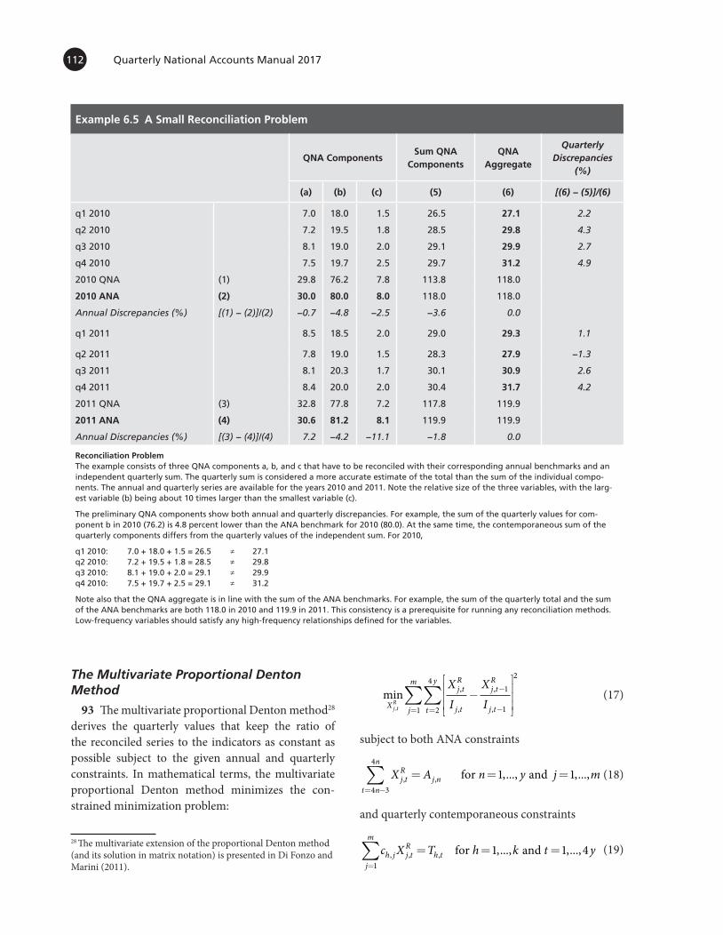
Quarterly National Accounts Manual 2017112
The Multivariate Proportional Denton Method
93 The multivariate proportional Denton method28 derives the quarterly values that keep the ratio of the reconciled series to the indicators as constant as possible subject to the given annual and quarterly constraints. In mathematical terms, the multivariate proportional Denton method minimizes the con-strained minimization problem:
28 The multivariate extension of the proportional Denton method (and its solution in matrix notation) is presented in Di Fonzo and Marini (2011).
min,
,
,
,
,X
j tR
j t
j tR
j tt
y
j
m
j tR
XI
XI
−
−
−==∑∑ 1
1
2
2
4
1
(17)
subject to both ANA constraints
X A n y j mj tR
j nt n
n
, , ,..., ,...,= = == −∑
4 3
4
1 1for and (18)
and quarterly contemporaneous constraints
c X T h k t yh j j tR
h tj
m
, , , ,..., ,...,= = ==∑
1
1 1 4for and (19)
Example 6.5 A Small Reconciliation Problem
QNA ComponentsSum QNA
ComponentsQNA
Aggregate
Quarterly Discrepancies
(%)
(a) (b) (c) (5) (6) [(6) − (5)]/(6)
q1 2010 7.0 18.0 1.5 26.5 27.1 2.2
q2 2010 7.2 19.5 1.8 28.5 29.8 4.3
q3 2010 8.1 19.0 2.0 29.1 29.9 2.7
q4 2010 7.5 19.7 2.5 29.7 31.2 4.9
2010 QNA (1) 29.8 76.2 7.8 113.8 118.0
2010 ANA (2) 30.0 80.0 8.0 118.0 118.0
Annual Discrepancies (%) [(1) − (2)]/(2) −0.7 −4.8 −2.5 −3.6 0.0
q1 2011 8.5 18.5 2.0 29.0 29.3 1.1
q2 2011 7.8 19.0 1.5 28.3 27.9 −1.3
q3 2011 8.1 20.3 1.7 30.1 30.9 2.6
q4 2011 8.4 20.0 2.0 30.4 31.7 4.2
2011 QNA (3) 32.8 77.8 7.2 117.8 119.9
2011 ANA (4) 30.6 81.2 8.1 119.9 119.9
Annual Discrepancies (%) [(3) − (4)]/(4) 7.2 −4.2 −11.1 −1.8 0.0
Reconciliation Problem The example consists of three QNA components a, b, and c that have to be reconciled with their corresponding annual benchmarks and an independent quarterly sum. The quarterly sum is considered a more accurate estimate of the total than the sum of the individual compo-nents. The annual and quarterly series are available for the years 2010 and 2011. Note the relative size of the three variables, with the larg-est variable (b) being about 10 times larger than the smallest variable (c).
The preliminary QNA components show both annual and quarterly discrepancies. For example, the sum of the quarterly values for com-ponent b in 2010 (76.2) is 4.8 percent lower than the ANA benchmark for 2010 (80.0). At the same time, the contemporaneous sum of the quarterly components differs from the quarterly values of the independent sum. For 2010,
q1 2010: 7.0 + 18.0 + 1.5 = 26.5 ≠ 27.1 q2 2010: 7.2 + 19.5 + 1.8 = 28.5 ≠ 29.8 q3 2010: 8.1 + 19.0 + 2.0 = 29.1 ≠ 29.9 q4 2010: 7.5 + 19.7 + 2.5 = 29.1 ≠ 31.2
Note also that the QNA aggregate is in line with the sum of the ANA benchmarks. For example, the sum of the quarterly total and the sum of the ANA benchmarks are both 118.0 in 2010 and 119.9 in 2011. This consistency is a prerequisite for running any reconciliation methods. Low-frequency variables should satisfy any high-frequency relationships defined for the variables.
6240-082-FullBook.indb 112 10/18/2017 6:09:14 PM

Benchmarking and Reconciliation 113
where
m is the number of QNA series in the system to be adjusted,
j is the generic index for a QNA series,
k is the number of quarterly relationships between the QNA series,
h is the generic index for a quarterly relationship,
X j tR, is the level of the QNA reconciled series j for
quarter t,
I j t, is the level of the quarterly indicator j for quarter t,
Aj n, is the level of the ANA benchmark j for year n,
ch j, is the coefficient of component j in the quarterly constraint h,
Th t, is the level of the quarterly constraint h for quar-ter t, and
t, n, and y are defined in equation (2).
94 The target values of the constrained mini-mization problem (equations (17)–(19)) are the quarterly values of the m series of the QNA sys-tem (specifically a total of 4y m⋅ values to be de-
termined). The penalty function is designed to preserve the overall movement in the indicators used in the QNA system. The minimization prob-lem allows for as many quarterly relationships as are established between the QNA series (for a single quarterly relationship, k = 1).
95 Coefficients ch j, and the constraint values Th t, , for h k=1,..., , define the type of quarterly relation-ships between the variables. For example, when the sum of QNA components (e.g., value added by eco-nomic activity) matches an independently derived aggregate estimate (e.g., value added by institutional sector), the values ch j, are equal to 1 for any j and Th t, is the value of the aggregate estimate for quarter t. For national accounts applications, the values of ch j, can be 1 (addition to the aggregate), −1 (sub-traction to the aggregate), or 0 (not included in the aggregate).
96 As for benchmarking, the reconciled series X j t
R, are derived as the solution of the constrained
minimization problem (equations (17)−(19)). The multivariate Denton method is illustrated in Example 6.6.
Example 6.6 The Multivariate Proportional Denton Method
Reconciled QNA ComponentsSum QNA
Components QNA AggregateQuarterly
Discrepancies (%)
(a) (b) (c) (5) (6) [(6) − (5)]/(6)
q1 2010 7.1 18.5 1.5 27.1 27.1 0.0
q2 2010 7.3 20.6 1.8 29.8 29.8 0.0
q3 2010 8.1 19.8 2.0 29.9 29.9 0.0
q4 2010 7.4 21.1 2.6 31.2 31.2 0.0
2010 QNA 30.0 80.0 8.0 118.0 118.0
2010 ANA 30.0 80.0 8.0 118.0 118.0
q1 2011 8.1 19.1 2.2 29.3 29.3 0.0
q2 2011 7.2 19.1 1.7 27.9 27.9 0.0
q3 2011 7.5 21.4 1.9 30.9 30.9 0.0
q4 2011 7.8 21.6 2.3 31.7 31.7 0.0
2011 QNA 30.6 81.2 8.1 119.9 119.9
2011 ANA 30.6 81.2 8.1 119.9 119.9
Solution with the Multivariate Proportional Denton Method The multivariate proportional Denton method adjusts the QNA components to meet both temporal and cross-sectional benchmarks in one step. The ratios between the reconciled QNA components and the preliminary QNA indicators (reconciled-to-indicator ratios) are presented in Example 6.9. The annual discrepancies are removed in a way so that the overall movement in the preliminary estimates of the QNA com-ponents is preserved. The quarterly discrepancies are distributed in proportion to the size of the preliminary QNA variables. These charac-teristics are more visible by looking at the results of the two-step reconciliation procedure (presented in Examples 6.7. and 6.8), which is an approximation of the multivariate proportional Denton method.
6240-082-FullBook.indb 113 10/18/2017 6:09:15 PM

Quarterly National Accounts Manual 2017114
derived using the Denton method, movements in the indicator are already preserved in the X j t
B, . Therefore,
in the second step, there is no need to preserve again movements in the objective function. A simple least-squares adjustment of the X j t
B, values is sufficient
to fulfill both the annual and quarterly constraints. Moreover, this adjustment can be done for each year separately, because the movement between one year and the next is already preserved by the bench-marked series.
100 Taking a generic year n, the second step is given by the least-squares solution of the constrained minimization:
min,
, ,
,X
j tR
j tB
j tB
t n
n
j
m
j tR
X X
X
−
= −=
∑∑2
4 3
4
1
(22)
subject to
X A n yj tR
j nt n
n
, , , ...,= == −∑
4 3
4
1for (23)
and
c X T
h k t n n
h j j tR
h tj
m
, , ,
,..., ,...,
=
= = −=∑
1
1 4 3 4for and (24)
where
X j tR, is the level of the QNA reconciled series j for
quarter t that satisfy both the corresponding ANA benchmarks Aj n, and the quarterly ac-counting relationships.
101 Penalty function (22) shows that the discrep-ancies ( ), ,X Xj t
Rj tB− are distributed in proportion to
the level of the benchmarked series.30 The relative size of the variables determines the amount of dis-crepancy to be distributed. The largest variables are
30 From a statistical viewpoint, taking the level of the bench-marked series at the denominator in function corresponds to assuming equal reliability of all variables (notwithstanding their relative size). An alternative solution for the second step has been suggested in Quenneville and Rancourt (2005), which takes the square root of the benchmarked series as normalizing factor of the discrepancy ( ), ,X Xj t
Rj tB− . This assumption assumes that large
variables are relatively more reliable than small variables, and therefore are touched less in the second step of the procedure.
A Two-Step Reconciliation Procedure
97 When the dimension of the system is too large, it could become time consuming, or even inefficient, to solve the constrained minimization problem (equations (17)–(19)). A convenient ap-proximation of the multivariate Denton method can be achieved using the following two-step procedure:29
· Benchmarking each of the m indicators to the corresponding ANA benchmarks using the uni-variate proportional Denton method. The first step provides temporally consistent QNA series, but it is likely to leave inconsistency in the quar-terly benchmarked series toward the quarterly accounting constraints.
· For each year separately, balancing the quarterly benchmarked series obtained at the first step to both annual and quarterly constraints relevant to the year. The balancing procedure is performed using a least-square adjustment. The second step splits the full system observed over the available span of years into y small systems covering one year at a time.
98 The first step is straightforwardly achieved by applying the univariate Denton method to the m variables in the system: that is, by solving the m con-strained minimization problems:
min,
,
,
,
,X
j tB
j t
j tB
j tt
q
j tB
XI
XI
−
−
−=∑ 1
1
2
2
for j m=1,..., (20)
subject to
X A n yj tB
j nt n
n
, , ,...,= == −∑
4 3
4
1for . (21)
where
X j tB, is the level of the QNA benchmarked series j for
quarter t to the corresponding ANA benchmarks.
99 The second step is needed to restore the con-temporaneous consistency in the benchmarked se-ries X j t
B, obtained at the first step. Because they are
29 Two-step reconciliation procedures are discussed in Quenn-eville and Fortier (2012). The approximation of the multivariate Denton method of the proposed two-step solution is illustrated with real-life examples in Di Fonzo and Marini (2011).
6240-082-FullBook.indb 114 10/18/2017 6:09:17 PM
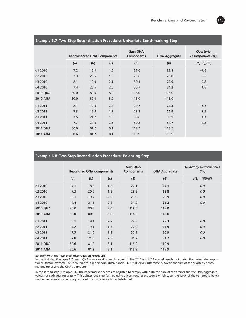
Benchmarking and Reconciliation 115
Example 6.7 Two-Step Reconciliation Procedure: Univariate Benchmarking Step
Benchmarked QNA ComponentsSum QNA
Components QNA AggregateQuarterly
Discrepancies (%)
(a) (b) (c) (5) (6) [(6) (5)]/(6)
q1 2010 7.2 18.9 1.5 27.6 27.1 −1.8
q2 2010 7.3 20.5 1.8 29.6 29.8 0.5
q3 2010 8.1 19.9 2.1 30.1 29.9 −0.8
q4 2010 7.4 20.6 2.6 30.7 31.2 1.8
2010 QNA 30.0 80.0 8.0 118.0 118.0
2010 ANA 30.0 80.0 8.0 118.0 118.0
q1 2011 8.1 19.3 2.2 29.7 29.3 −1.1
q2 2011 7.3 19.8 1.7 28.8 27.9 −3.2
q3 2011 7.5 21.2 1.9 30.6 30.9 1.1
q4 2011 7.7 20.8 2.3 30.8 31.7 2.8
2011 QNA 30.6 81.2 8.1 119.9 119.9
2011 ANA 30.6 81.2 8.1 119.9 119.9
Example 6.8 Two-Step Reconciliation Procedure: Balancing Step
Reconciled QNA ComponentsSum QNA
Components QNA AggregateQuarterly Discrepancies
(%)
(a) (b) (c) (5) (6) [(6) − (5)]/(6)
q1 2010 7.1 18.5 1.5 27.1 27.1 0.0
q2 2010 7.3 20.6 1.8 29.8 29.8 0.0
q3 2010 8.1 19.7 2.0 29.9 29.9 0.0
q4 2010 7.4 21.1 2.6 31.2 31.2 0.0
2010 QNA 30.0 80.0 8.0 118.0 118.0
2010 ANA 30.0 80.0 8.0 118.0 118.0
q1 2011 8.1 19.1 2.2 29.3 29.3 0.0
q2 2011 7.2 19.1 1.7 27.9 27.9 0.0
q3 2011 7.5 21.5 1.9 30.9 30.9 0.0
q4 2011 7.8 21.6 2.3 31.7 31.7 0.0
2011 QNA 30.6 81.2 8.1 119.9 119.9
2011 ANA 30.6 81.2 8.1 119.9 119.9
Solution with the Two-Step Reconciliation Procedure In the first step (Example 6.7), each QNA component is benchmarked to the 2010 and 2011 annual benchmarks using the univariate propor-tional Denton method. This step removes the temporal discrepancies, but still leaves difference between the sum of the quarterly bench-marked series and the QNA aggregate.
In the second step (Example 6.8), the benchmarked series are adjusted to comply with both the annual constraints and the QNA aggregate values for each year separately. This adjustment is performed using a least-squares procedure which takes the value of the temporally bench-marked series as a normalizing factor of the discrepancy to be distributed.
6240-082-FullBook.indb 115 10/18/2017 6:09:17 PM

Quarterly National Accounts Manual 2017116
• When quarterly indicators are of inferior quality than annual data, benchmarking methods should be used to derive QNA series that (i) are temporally consistent with the ANA benchmarks, (ii) preserve as much as possible the quarterly movements in the indicators, and (iii) provide accurate extrapolations for the current year.
• The pro rata method is not an appropriate method for benchmarking QNA series, because it may distort the quarter-to-quarter movement in the first quarter of each year.
• The preferred option for benchmarking QNA series is the proportional Denton method. The enhanced Denton formula for extrapolation could be used in place of the basic Denton method to improve the QNA estimates for the current year. This method requires a forecast of the next annual BI ratio, which should be determined exter-nally by the user looking at the development of the annual BI ratio series.
• As an alternative to the Denton method, the proportional Cholette–Dagum method with first-order AR error could be used to obtain bias-adjusted QNA extrapolations based on historical behavior. The recommended value of the AR parameter is 0.84, or alternatively chosen in a range between 0.71 and 0.93, depending on the move-
Example 6.9 Results from Multivariate Denton Method and Two-Step Procedure
Multivariate Denton Method Two-Step Reconciliation Procedure
Reconciled-to-Indicator Ratios
Reconciled-to-Indicator Ratios
Benchmarking Step (BI Ratios)
Balancing Step (Reconciled-to-
Benchmark Ratios)
(a) (b) (c) (a) (b) (c) (a) (b) (c) (a) (b) (c)
q1 2010 1.016 1.027 0.998 1.015 1.027 0.999 1.024 1.051 1.002 0.992 0.977 0.998
q2 2010 1.020 1.057 1.009 1.020 1.058 1.009 1.017 1.051 1.009 1.003 1.006 1.000
q3 2010 1.000 1.040 1.024 1.001 1.039 1.024 1.004 1.050 1.026 0.997 0.990 0.998
q4 2010 0.993 1.073 1.055 0.993 1.073 1.055 0.984 1.048 1.052 1.009 1.024 1.002
q1 2011 0.950 1.031 1.090 0.951 1.031 1.089 0.957 1.046 1.091 0.994 0.985 0.998
q2 2011 0.920 1.004 1.116 0.923 1.003 1.115 0.936 1.044 1.120 0.986 0.961 0.996
q3 2011 0.929 1.057 1.140 0.928 1.057 1.141 0.923 1.043 1.140 1.005 1.014 1.001
q4 2011 0.932 1.080 1.153 0.929 1.081 1.155 0.916 1.042 1.150 1.014 1.037 1.004
Reconciled-to-Indicator Ratios The reconciled-to-indicator ratios of the multivariate Denton method and of the two-step reconciliation procedure are presented in the table. It can be seen that the ratios of the two-step procedure are very close to those from the multivariate Denton approach.
The table also presents the ratios of the benchmarked series to the indicator series obtained at the first step (i.e., the BI ratio) and the ratios of the reconciled series obtained at the second step and the benchmarked series obtained at the first step (reconciled-to-benchmark ratios). As seen in the benchmarking section, the BI ratios obtained using the Denton method move smoothly between the quarters. Instead, the reconciled-to-benchmark ratios show that the quarterly discrepancies—reported in the last three columns of Example 6.9—are distributed in proportion to the size of the variable. In fact, most of the quarterly discrepancy for each quarter is assigned to component b, which is the largest variable in the system, while component c gets the smallest portion.
Summary of Key Recommendations
those receiving the highest portion of contempora-neous discrepancy.
102 The solutions to systems (equations (22)–(24)) for all the available years (i.e., n y=1,..., ) generate quarterly reconciled series X j t
R, that are
close approximations of the optimal solution provided by the multivariate Denton propor-
tional method. An illustration of the two-step procedure is given in Examples 6.7 and 6.8. The results from the multivariate Denton method and the two-step procedure are compared in Exam-ple 6.9 using the ratios between the reconciled series X j t
R, , the benchmarked series X j t
B, , and the
indicators I j t, .
6240-082-FullBook.indb 116 10/18/2017 6:09:18 PM

Benchmarking and Reconciliation 117
ments in the BI ratio. These values guarantee that movements in the indicator are adequately preserved for the back series.
• The Denton method and Cholette–Dagum method should be tested on the specific benchmarking cases in the QNA. The method providing the most accurate results should be chosen. Ultimately, the choice between the two methods could be a subjective call. The same method should be used for calculating both the back series and the forward series of the same variable. Once a method is chosen for a variable, the method should be used consis-tently over time.
• For reconciliation problems, the multivariate proportional Denton method should be used for deriving a system of QNA series subject to both annual and quarterly constraints.
• When the dimension of the QNA system is too large to be solved efficiently in one step, the following two-step procedure may be used to approximate the optimal results of the multivariate Denton method:
• benchmarking each quarterly indicator to the corresponding ANA benchmarks using the proportional Denton method and
• for each year separately, balancing the quarterly benchmarked series obtained at the first step using a least-squares procedure that proportionally adjusts the original values to realign them with both annual and quar-terly constraints relevant to the year.
6240-082-FullBook.indb 117 10/18/2017 6:09:18 PM

1 Benchmarking refers to the procedures used to maintain consistency among the time series available at different frequencies for the same target variable. In the QNA, benchmarking usually consists of ad-justing quarterly data to match annual (or quinquen-nial) benchmarks. 31 Quarterly values of indicators are modified so that the annual sums (or average) of the adjusted values are equal to the corresponding ANA benchmarks, which are considered the more compre-hensive and accurate measurement in level of national accounts variables.
2 Benchmarking methods can be grouped into two main approaches: the numerical approach and the model-based approach. Numerical methods de-termine the target values as the solution of an ad hoc constrained optimization problem, where an objec-tive function is defined to preserve some characteris-tics of the original information available. Examples of numerical methods preserving the movements in the indicator are the benchmarking methods proposed by Denton (1971) and Monsour and Trager (1979). This group also includes mathematical solutions to decom-pose annual data into consistent quarterly data with-out the use of a quarterly related indicator, such as the methods by Lisman and Sandee (1964) and Boot, Feibes and Lisman (1967).
3 Model-based benchmarking methods perform the adjustment under the assumption of a statisti-cal model for the unknown values to be determined. Model-based benchmarking methods encompass ARIMA32 model-based methods of Hillmer and Tra-belsi (1987), regression-based methods proposed by Cholette and Dagum (1994), and state space models of Durbin and Quenneville (1997). In addition, Chow and Lin (1971) proposed a multivariable general least-squares regression approach for interpolation, distri-bution, and extrapolation of time series. 33 While not
31 The term “benchmarking” was first introduced in Helfand, Monsour, and Trager (1977) to describe the historical revision of monthly survey data to incorporate census benchmarks every five years.32 Autoregressive-integrated moving average.33 Related works to the Chow–Lin solution are Fernández (1981), Litterman (1983), and Wei and Stram (1990).
a benchmarking method in a strict sense, the Chow–Lin method is related to the regression-based model developed by Cholette and Dagum (as explained later in this annex).
4 This annex provides a brief review of benchmark-ing methods for compiling QNA. The annex is not in-tended to provide an extensive survey of all alternative benchmarking methods proposed in the literature.34 The aim of this annex is to offer a more technical dis-cussion of the two benchmarking methods identified in the chapter as suitable for QNA purposes: namely,
· The benchmarking method proposed by Denton (1971), with its enhancement for extrapolation. The Denton proportional method is the pre-ferred option for benchmarking. The enhanced version should be used for extrapolation when a forecast of the next annual BI ratio is available.
· The regression-based benchmarking method proposed by Cholette and Dagum (1994). An al-ternative solution to the Denton approach is the proportional Cholette–Dagum method with AR extrapolation, which preserves the movements in the indicator for the back series and automati-cally adjusts QNA extrapolations for a temporary bias in the indicator.
5 This annex illustrates the two benchmarking meth-ods mentioned above using a standardized formal no-tation. Each method (including the Cholette–Dagum approach) can be interpreted as the solution to a con-strained minimization problem under a specific ob-jective (or penalty) function. Further details for each method will be highlighted in both distribution and extrapolation steps. Finally, solutions of both methods are presented in matrix notation. Conveniently, a ma-trix representation permits to express the constrained minimization problem as a linear system and derive the benchmarked series as (part of) its solution using simple algebra operations. The technical presentation provided in this annex is intended to facilitate the implementa-tion of these benchmarking methods in any preferred programming language with matrix capabilities.
34 For further reference, see Dagum and Cholette (2006).
Annex 6.1 Benchmarking Methods
6240-082-FullBook.indb 118 10/18/2017 6:09:18 PM

Benchmarking and Reconciliation 119
6 The annex presents briefly the regression-based benchmarking (or temporal disaggregation) method proposed by Chow and Lin (1971). The Chow–Lin ap-proach is presently used in many countries for com-piling QNA variables. The annex explains how the Chow–Lin method relates to the Denton and Cho-lette–Dagum methods.
The Denton Benchmarking Method
7 Denton (1971) proposed a method to adjust quar-terly (or monthly) series so that the annual sums of the adjusted values are equal to independent annual totals and the resulting quarterly series be free of artificial dis-continuities between the years. The adjustment method proposed by Denton (later became known as bench-marking) is grounded on a principle of movement preservation, whereby the adjusted values are sought to preserve maximally the movement in the original se-ries. The adjustment follows thus a purely mechanical scheme, with no explicit statistical models or assump-tion describing the behavior of the series involved. The Denton benchmarking method has become popular in the QNA and in other areas of official statistics for its easy implementation and its flexibility and robustness to handle different kinds of benchmarking problems.
8 Denton formulated the benchmarking prob-lem as a constrained quadratic minimization of a penalty function, designed to minimize the impact of the adjustment on the movements in the original values. Denton proposed two penalty functions: an additive solution and a proportional solution. 35 They are shown below with the modifications proposed by Cholette (1984) to deal with the starting condition: 36
· Additive First Difference (AFD) Function
min [( ) ( )]
min [( ) (
X t t t tt
y
X t t t t
t
t
X I X I
X X I I
− − − ⇔
− − −
− −=
− −
∑ 1 12
2
4
1 1))]2
2
4
t
y
=∑
(A1)
35 Denton also proposed additive and proportional solutions that minimize the impact on second or higher-order differences in the original series. The proportional second difference solution is particularly convenient with stock variables, as discussed in Dagum and Cholette (2006). 36 The original proposal by Denton assumed that the value for the first period of the series was predetermined. For more details on the original Denton method and the modified solution for the starting condition, see Dagum and Cholette (2006, chapter 6).
· Proportional First Difference (PFD) Function
min
min
Xt t
t
t t
tt
y
Xt
t
t
t
t
q
X II
X II
XI
XI
−−
−
⇔
−
− −
−=
−
∑ 1 1
1
2
2
4
1
−−=
∑
1
2
2
4
t
y (A2)
where
Xt is the quarterly series to be calculated (i.e., the QNA series),37
It is the quarterly series available (i.e., the indicator), An is the annual series to be fulfilled (i.e., the ANA
benchmarks), t y=1 4,..., is the temporal index for the quarters, and n y=1,..., is the index for the years.
Quarterly observations are available for each year. As shown later, the method can be extended easily to cover the case of extrapolation in quarters beyond the last available annual benchmark.
9 Formulas (A1) and (A2) are minimized under the same restrictions, which for flow series correspond to
X A n yt nt n
n
= == −∑ , , ...,1
4 3
4
(A3)
that is, the sum of the quarters must be equal to an-nual benchmarks available for each year. Annual benchmarks An are binding (or “hard”) constraints in the system, as they cannot vary in the adjustment pro-cess. The Denton approach does not allow nonbind-ing (or “soft”) benchmarks, a distinguished feature of the Cholette–Dagum regression-based model that is illustrated later in the annex.
10 The PFD variant (equation (A2))—indicated in this chapter as proportional Denton method—is gen-erally preferred over the AFD formula (A1) because it preserves seasonal and other short-term fluctuations in the series better when these fluctuations are multi-plicatively distributed around the trend of the series. Multiplicatively distributed short-term fluctuations seem to be characteristic of most seasonal macro-economic series. By the same token, it seems most
37 The present formulation assumes that both the annual and quarterly observations are contiguous (no missing values) and that each annual benchmark is covered by the corresponding quarterly figures of the indicator.
6240-082-FullBook.indb 119 10/18/2017 6:09:19 PM

Quarterly National Accounts Manual 2017120
reasonable to assume that the errors are generally multiplicatively, and not additively, distributed, un-less anything to the contrary is explicitly known. The additive formula results in a smooth additive distribu-tion of the errors in the indicator, in contrast to the smooth multiplicative distribution produced by the proportional formula. Consequently, the additive ad-justment tends to smooth away some of the quarter-to-quarter rates of change in the indicator series. As a result, the additive formula can seriously disturb that aspect of the short-term movements for series that show strong short-term variations. This can occur particularly if there is a substantial difference between the level of the indicator and the target variable. In addition, the AFD formula may in a few instances re-sult in negative benchmarked values for some quar-ters (even if all original quarterly and annual data are positive) if large negative adjustments are required for data with strong seasonal variations.
11 The proportional variant of the Denton method does not preserve explicitly the quarterly rates of change of the indicator, which are commonly taken by users to analyze the short-term dynamics of eco-nomic series. A more explicit penalty function based on quarterly rates of change can be defined as follows:
min
min
Xt t
t
t t
tt
y
Xt
t
t
t
t
X XX
I II
XX
I
−−−
⇔
−
−
−
−
−=
−
∑ 1
1
1
1
2
2
4
1 IItt
y
−=
∑
1
2
2
4
,
(A4)
which is known in the literature as growth rates pres-ervation (GRP) principle. The PFD function proposed by Denton, however, is a very close approximation of the GRP,38 in particular when the BI ratio does not present sudden jumps from one year to the next and the indicator is not too volatile. Furthermore the GRP function (A4) is a (quadratic) nonlinear function of the objective values (because Xt−1 appears at the de-nominator of the ratio) and therefore its first-order conditions do not give rise to an explicit algebraic solution for the linear system. Nonlinear optimiza-tion procedures are required to find the benchmarked values minimizing the GRP function. Modern tech-
38 It can be shown that the term of the PFD function is equal to the term of the GRP function multiplied by the ratio ( )X It t−1
2 (see Di Fonzo and Marini, 2013).
nology may consent an efficient implementation39 of a GRP-based benchmarking procedure; however, performance of nonlinear solvers depends on the particular benchmarking problem faced and it is not possible to exclude slow convergence rates and inac-curate results in finding the actual minimum of the GRP function. For this reason, the proportional Den-ton method represents the most convenient solution for QNA compilers to preserve the quarter-to-quarter growth rates in the indicator.
12 As shown by formula (A2), the proportional Denton solution amounts to minimizing the sum of the squared first differences of the quarterly BI ratio: that is, the ratio between the (unknown) bench-marked series Xt and the (known) indicator It. This chapter notes that the BI framework allows a useful interpretation of the proportional Denton method. The proportional technique implicitly constructs from the annual observed BI ratios a time series of quarterly BI ratios that are as smooth as possible. In the case of flow series, quarterly BI ratios for the back series (n y=1,..., ) are derived as weighted average of the annual BI ratios for each year n: that is,
XI
wAI
t
tt n
n
tn
n= −∑ =
4 3
4
with
I In tt n
n
== −∑
4 3
4
the annual sums of the quarterly obser-
vations and
wI
It
t
tn
n=
−∑4 3
4 the indicator’s weight for each quarter
of the year, for t n n= −4 3 4,..., .
13 The original method proposed by Denton (1971) did not consider the problem of extrapolat-ing quarterly values for the year(s) following the last available annual observation. However, this extension is straightforward. Formulas (A1) and (A2) still work
39 Causey and Trager (1981) and Brown (2010) used gradient-based algorithms to minimize the growth rate preservation (GRP). Di Fonzo and Marini (2012a) proposed an interior point-based procedure, which makes use of second-order derivative information to increase robustness and efficiency in achieving the minimum value of the GRP function.
6240-082-FullBook.indb 120 10/18/2017 6:09:20 PM

Benchmarking and Reconciliation 121
when the indicator It is observed for t y= +4 1,.... No additional constraints is needed for the quarterly values of the year y+1, since the annual benchmark from the ANA is yet unknown. To minimize the PFD function, the extrapolated quarters are derived by as-suming that the BI ratio is constant and equal to the last available quarterly BI ratio: that is, the fourth quarter of the year y in the current notation
XI
XI
y k
y k
y
y
4
4
4
4
+
+
= , for k≥1.
14 Forwarding the last available quarterly BI ratio using the proportional Denton method may lead to inaccurate extrapolation. It is possible to improve the estimates for the most recent quarters (i.e., the for-ward series) and reduce the size of later revisions by incorporating information on past systematic move-ments in the annual BI ratio. It is important to im-prove the estimates for these quarters, because they are typically of the keenest interest to users. Carrying forward the quarterly BI ratio from the last quarter of the last year is an implicit forecast of the annual BI ratio, but a better forecast may be derived observing the development of the annual BI ratio for the avail-able years.
15 To produce extrapolations that are consistent with a forecast of the next annual BI ratio, the same principles of constrained minimization used in the Denton formula can be used. Since the benchmark value is unavailable, the annual constraint is formu-lated in a way such that the weighted average of the quarterly BI ratios is equal to the forecast of annual BI ratio.
16 Denote with by+1 the annual BI ratio of the year to extrapolate,
bAIy
y
y+
+
+
=11
1
where I Iy tt y
t y
+= + −
= +
= ∑14 1 3
4 1
( )
( )
.
Suppose the indicator’s quarterly values are available for the year y+1: namely, I I I Iy y y y4 1 4 2 4 3 4 1+ + + +, , , ..., ( ). In mathematical terms, the enhanced proportional Denton method becomes the solution to the follow-ing constrained minimization problem:
min( )
Xt
t
t
tt
y
t
XI
XI
−
−
−=
+
∑ 1
1
2
2
4 1
(A5)
subject to the annual benchmarks for the years n y=1,...,
X At nt n
n
== −∑
4 3
4
and, for the next year y+1, to the forecast of the an-nual BI ratio
XI
w bt
tt y
t y
y
− += + −
+
=∑ 4 14 1 3
4 1ˆ
( )
( )
where
w I It t tt n
n
== −∑
4 3
4
are the indicator’s quarterly shares
of a year and
byˆ+1 is the annual forecast of the BI ratio for the year
y+1 .
Matrix Solution of the Proportional Denton Method
17 The Denton benchmarking problem can be rewritten in matrix notation. This representation is convenient to calculate the benchmarked series with simple matrix operations. Assume there are no extrapolations (q y= 4 ). In matrix form, the minimization problem defined by equation (A2) under the constraint equation (A3) can be ex-pressed as
minX
X I M X I−( )′ −( ) (A6)
subject to
JX A= , (A7)
where
X is the ( )4 1y× vector containing the values Xt of the benchmarked series;
I is the ( )4 1y× vector with the values It of the indicator;
A is the ( )y×1 vector with the annual benchmarks At; J is the ( )y y×4 matrix aggregating 4y contiguous
quarterly data into the corresponding y annual data,
6240-082-FullBook.indb 121 10/18/2017 6:09:24 PM

Quarterly National Accounts Manual 2017122
J=
1 1 1 1 0 0 0 0
0 0 0 0 1 1 1 1
…
…;40 (A8)
M = I D D I-1 -1ˆ ˆ′( ) ;
I is the ( )4 4y y× diagonal matrix containing the val-ues of the indicator in the main diagonal,
I=
II
I y
1
2
4
0 00 0
0 0
...
...
...
; and
D is the ( )4 1 4y y− × matrix calculating the first dif-ference from q-dimensional vectors,
D=
−−
1 1 0 00 1 1
0 0 0 1
…
… …
…
.
18 Constrained quadratic minimization problem (A6) is solved by calculating the first-order condi-tions for a minimum, namely by equating to zero the partial derivatives of (A2) with respect to Xt and the Lagrange multipliers of the system. The two equations generate the following linear system:
M JJ 0
X MIA
′
=
y λ
where 0y is the zero matrix of dimension y.
The solution is achieved by simple inverse and multi-plication operations of the matrices involved:
X M JJ 0
MIA
-1ˆ
λ
′
= . (A9)
The ( )q×1 vector X in the left-hand side of equation (A9), which is (part of) the solution to the linear sys-
40 For flow series with regularly spaced years and quarters, ma-trix J can be derived as I 1y ⊗ , where Iy is the identity matrix of dimension y, 1 is a 1 4× row vector of ones, and ⊗ is the Kronecker product.
tem (equation (A6)), contains the benchmarked val-ues of the proportional Denton method.41
19 To obtain extrapolations (case q y≥ 4 ), the only adjustments to the above formulation are to extend matrix J with as many zero columns as the number of extrapolations required and include the values of the indicator up to the last quarterly observation avail-able. For example, for the extrapolation of q1 of the next year (q y= +4 1),
J=
1 1 1 1 0 0 0 0 0
0 0 0 0 1 1 1 1 0
…
…
and
I=
+
II
II
y
y
1
2
4
4 1
0 0 00 0 0
0 0 00 0 0
...
...
...
...
.
The Cholette–Dagum Regression-Based Method
20 Cholette and Dagum (1994) proposed a bench-marking method based on the generalized least-squares regression model. The Cholette–Dagum model takes into account (i) the presence of bias in the indicator and (ii) the presence of autocorrelation and heteroscedasticity errors in the original data. In addition, it allows for nonbinding benchmarks. These characteristics make the Cholette–Dagum approach a very flexible benchmarking framework. The Denton method can be seen as a particular (approximated) case of the Cholette–Dagum regression model.
21 The benchmarking method proposed by Cho-lette and Dagum (1994) is based on the following two equations42:
I a X et t t t= + + for t q=1,..., (A10)
A X wn tt n
n
n= += −∑
4 3
4
for n y=1,.., (A11)
41 The matrix solution of the enhanced Denton proportional solu-tion can be found in Di Fonzo and Marini (2012b)42 This presentation of the Cholette–Dagum model assumes that both the annual and quarterly observations are contiguous (no missing values) and that each annual benchmark is covered by the corresponding quarterly figures of the indicator.
6240-082-FullBook.indb 122 10/18/2017 6:09:27 PM

Benchmarking and Reconciliation 123
where
It is the quarterly series available (i.e., the QNA indicator),
at is a (combined) deterministic effect,
Xt is the true quarterly series,
et is a quarterly autocorrelated and heteroscedastic43 error, and
wn is an annual heteroscedastic error in the annual series An , uncorrelated with et,
with
E e E e et t t h( ) , ( )= ≠−0 0
E w E wn n n( ) , ( )= =0 2 2δ
E e wt n( )= 0.
22 The proportional Cholette–Dagum method with AR error can be used to improve QNA extrapo-lations. This annex shows the assumptions that define this specific option from the general Cholette–Dagum regression-based framework defined by equations (A10) and (A11), and provides the solution in matrix notation for its implementation.
23 Equation (A10) describes the values of the quarterly indicator It as a measure of variable Xt con-taminated with deterministic effect at and quarterly error et. Equation (A11) relates the annual benchmark An to the annual sum of the quarterly values Xt with a possible measurement error wn. The Cholette–Dagum regression-based method varies according to the as-sumptions for the deterministic effect at, the quarterly error et, and the annual error wt.
24 The annual error wt is needed to account for situations whether the benchmark is also subject to error. These benchmarks are called nonbinding, be-cause they are also subject to changes in the bench-marking process. In the QNA, however, the annual benchmarks are usually binding constraints for the quarterly values (i.e., E wn( )2 0= ).
25 The deterministic effect at is usually calculated from a set of deterministic regressors rt h, multiplied by their corresponding regression coefficients βh: that is,
43 Autocorrelation refers to the correlation of the error with its own past and future. Heteroscedasticity means that the variance of the error varies across observations.
a rt t h hh
s
==∑ , β
1
,
where s is the number of deterministic effects consid-ered. A constant is a typical deterministic effect used to capture a level bias difference between the annual and the quarterly level. As explained in the chapter, a constant bias can also be modeled implicitly by rescal-ing the original indicator with the historical BI ratio. This transformation is convenient because it requires no parameter estimation of the level bias. A deter-ministic trend could also be used to catch a diverging path between the indicator and the objective variable. However, deterministic trend may cause biased ex-trapolations at both ends of the series and should be used with caution.
26 The error et is the quarterly discrepancy be-tween the target variable Xt and the quarterly indi-cator It . Because a key objective of benchmarking is to keep the movements in Xt as close as possible to the movements in It, the error et needs to have two characteristics:
· It has to be proportional to the value of the indicator It . This property is necessary to dis-tribute the errors around the level of the in-dicator, similar to the proportional Denton solution.
· It has to present smooth movements from one quarter to the next. A smooth distribution of et make the movements of Xt and It very close to each other.
27 To obtain a proportional adjustment, the error et is standardized by the value of the indicator It ,
′ =eeIt
t
t
. (A12)
By doing so, the standard deviation of et is assumed to be equal to It .44 To obtain a smooth distribu-tion, the standardized error ′et is assumed to follow a first-order (stationary) autoregressive model, or AR(1) model:
′ = ′ +−e e vt t tφ 1 (A13)
44 This assumption implies constant coefficient of variations: that is, σt tI/ = 1 for any quarter t.
6240-082-FullBook.indb 123 10/18/2017 6:09:31 PM

Quarterly National Accounts Manual 2017124
with φ <1 , where the vt ’s are assumed to be indepen-dent and identically distributed innovations: that is,
E v E v E v vt t t t h( ) , ( ) , ( , )= = =−0 1 02 for any t and h.
28 The proportional Cholette–Dagum method with AR error entails the minimization of an objective function that is closely related to the proportional cri-terion (equation (A2)) minimized by Denton. It can be shown that the benchmarked series of the propor-tional Cholette–Dagum model with AR error model (A13) minimizes the objective function45:
minX a
t
ta
t
ta
t
XI
XI
XI
11 2
1
1
21
1−
+ − −
−φφ
=
∑t
q
2
2
. (A14)
29 Function (A14) clarifies that, besides extrapo-lation, the AR parameter φ plays a crucial role in preserving the short-term dynamics of the indicator series. When φ is very close to 1 (e.g., 0.999), func-tion (A14) converges to function (A2),46 which is minimized by the proportional Denton method. As φ moves away from 1, the quarterly BI ratios are adjusted according to a criterion that offers weaker movement preservation than the Denton solution. For the reasons explained in the chapter, the value of φ should be chosen in a range between 0.71 and 0.93.
Matrix Solution of the Proportional Cholette–Dagum Method with AR Error
30 The solution to the Cholette–Dagum propor-tional benchmarking with AR error is given by the expression
X I VJ JVJ A JI= + ′ ′ −
−a a( ) 1 ,
where
X, A, and J are defined in equation (A6), Ia is the ( )q×1 vector with the bias-adjusted indica-
tor Ita calculated in equation (A11),
V = I Iˆ ˆa a( )-1Ω is the ( )q q× variance–covariance ma-trix of the quarterly error et ,
45 Dagum and Cholette (2006, pp. 87–92).46 The Denton method provides the same results whether the original indicator or the bias-adjusted indicator is used.
Ia is the ( )q q× diagonal matrix containing the values of the bias-adjusted indicator It
a in the main diagonal,
Ω= W W′ is the autocorrelation matrix of the AR(1) model with parameter φ, where
W=
−−
−
1 0 0 01 0 0
0 1 0
0 0 0 1
2φφ
φ
…
…
…
.
The Chow–Lin Regression-Based Method
31 Chow and Lin (1971) proposed a method for interpolating, distributing, and extrapolating time series based on a regression model using related in-dicators. The Chow–Lin method is presently used by many statistical agencies for compiling QNA. Given its widespread use in the QNA, this annex provides a brief description of this approach. In particular, this section illustrates the main features of the Chow–Lin method and relates this approach to the benchmark-ing methods proposed by Denton (1971) and Cholette and Dagum (1994).
32 The Chow–Lin method assumes a regression model between the true (unobserved) quarterly ob-servations Xt and a set of p quarterly related series I It p t1, ,, ..., :
X I ut j j t tj
p
= +=∑β ,
1
, for t q=1,..., (A15)
with
u u vt t t= +−ρ 1 , (A16)
where
Xt is the quarterly (unknown) target value (i.e., the QNA series);
β j is the regression coefficient for the j-th indicator;
I j t, is the j-th quarterly indicator;
ut is a random error assumed to follow the AR(1) model (A16), with the vt’s independently and identically distributed innovations; and
q is the number of quarters, possibly including ex-trapolations (q y≥ 4 ).
6240-082-FullBook.indb 124 10/18/2017 6:09:35 PM
Benchmarking and Reconciliation 125
33 Because Xt is unobserved (and its values are the target values of the method), model (A15) cannot be estimated. However, Chow and Lin assumes that the same relationship between Xt and the quarterly indicators holds true at the annual frequency. There-fore, model (A15) is temporally aggregated:
A I un j j n na
j
p
= +=∑β ,
1
, for n y=1,..., (A17)
where
A Xn tt n
n
== −∑
4 3
4
is the (known) annual variable that
needs to be distributed and extrapolated into quarters (i.e., the ANA benchmarks), β j is the regression coefficient for the j-th indicator
(assumed constant across frequencies),
I j n, is the j-th annually aggregated indicator, and
una is an annual ARMA(1,1) error derived from the
quarterly AR(1) model. 47
34 Chow and Lin derives the best linear unbiased estimator (BLUE) of Xt by estimating the regression coefficients β j and the AR coefficient ρ from model (A17). The estimated series Xt
ˆ (which corresponds to the benchmarked series) consists of two components:
one from the regression effects β j j tj
p
I ,=∑
1
and one from
the estimated quarterly residual utˆ . Regression effects may include deterministic effects (constant, trend, etc.) and related indicators. In the QNA, the most frequent combination of regressor is a constant term plus an indicator. The estimate ρ can be done by maxi-mum likelihood or by weighted least squares. Simi-lar to the AR error in the Cholette–Dagum method, the estimated value of ρ should be positive in order to preserve the original movements from the regression component.
35 Dagum and Cholette (2006) shows that the Chow–Lin model is a particular case of their regres-sion-based additive model with one related series. The AR(1) assumption for ut
48 is needed to distrib-
47 When temporally aggregated, an AR(1) model results in an ARMA (1,1) model. 48 Other assumptions for the quarterly error are the random walk model by Fernández (1981) and the AR(1)-plus-random walk model by Litterman (1983).
ute the quarterly errors smoothly, similar to the Cho-lette–Dagum method with AR error. However, in the Chow–Lin approach, the AR coefficient ρ is estimated from the data observed and not chosen by the user (as for the AR coefficient φ in the Cholette–Dagum model). Although this can be considered a good theoretical property of the model, the maximum likelihood estimation process may lead to negative estimates of ρ, and when this happens, the error com-ponent may dominate the short-term movements of the benchmarked series.
BibliographyBarcellan, R., and R. Buono (2002), “Temporal Disaggrega-
tion Techniques – ECOTRIM Interface (Version 1.01),” User Manual, Eurostat.
Boot, J.C.G., W. Feibes, and J.H.C. Lisman (1967), “Further Methods of Derivation of Quarterly Figures from Annual Data,” Applied Statistics, 16(1): 65–75.
Brown, I. (2010), “An Empirical Comparison of Con-strained Optimization Methods for Benchmarking Eco-nomic Time Series,” in Joint Statistical Meetings 2009 Proceedings, Business and Economic Statistics Section, pp. 2131–2143, Washington, DC: American Statistical Association.
Causey, B., and M.L. Trager (1981), “Derivation of Solution to the Benchmarking Problem: Trend Revision,” Unpub-lished Research Notes, U.S. Census Bureau.
Cholette, P. A. (1984), “Adjusting Sub-annual Series to Yearly Benchmarks,” Survey Methodology, 10: 35–49.
Cholette, P.A. (1994), “Users’ Manual of Programme BENCH,” Working Paper Time Series Research and Analysis Division, TSRA-90-009, Ottawa: Statistics Canada.
Cholette, P.A., and E.B. Dagum (1994), “Benchmarking Time Series with Autocorrelated Survey Errors,” Interna-tional Statistical Review, 62(3): 365–377.
Chow, G.C., and A. Lin (1971), “Best Linear Unbiased In-terpolation, Distribution, and Extrapolation of Times Series by Related Series,” The Review of Economic and Statistics, 53(4): 372–375.
Dagum, E.B., and P.A. Cholette (2006), Benchmarking, Temporal Disaggregation, and Reconciliation Methods for Time Series, Springer edition, New York: Springer.
Denton, F. (1971), “Adjustment of Monthly or Quarterly Se-ries to Annual Totals: An Approach based on Quadratic Minimization,” Journal of the American Statistical Asso-ciation, 66(333): 99–102.
6240-082-FullBook.indb 125 10/18/2017 6:09:36 PM

Quarterly National Accounts Manual 2017126
Di Fonzo, T., and M. Marini (2011), “Simultaneous and Two-Step Reconciliation of Systems of Time Series: Methodological and Practical Issues,” Journal of Royal Statistical Society: Series C, 60(2): 143–164.
Di Fonzo, T., and M. Marini (2012a), “Benchmarking Time Series According to a Growth Rates Preservation Princi-ple,” Journal of Economic and Social Measurement, 37(3): 225–252.
Di Fonzo, T., and M. Marini (2012b), “On the Extrapolation with the Denton Proportional Benchmarking Method,” IMF Working Paper Series, WP/12/169.
Di Fonzo, T., and M. Marini (2013), “Benchmarking and Movement Preservation: Evidences from Real-Life and Simulated Series,” in N. Torelli and others (eds), Advances in Theoretical and Applied Statistics, pp. 499–509, Heidel-berg: Springer-Verlag.
Durbin, J., and B. Quenneville (1997), “Benchmarking by State Space Models,” International Statistical Review, 65(1): 23–48.
Fernández, R.B. (1981), “A Methodological Note on the Es-timation of Time Series,” The Review of Economics and Statistics, 63(3): 471–476.
Helfand, S.D., N.J. Monsour, and M.L. Trager (1977), “His-torical Revision of Current Business Survey Estimates,” in Proceedings of the Business and Economic Statistics Sec-tion, American Statistical Association, Washington, DC, United States, pp. 246–250.
Hillmer, S.C., and A. Trabelsi (1987), “Benchmarking of Economic Time Series,” Journal of the American Statisti-cal Association, 82(400): 1064–1071.
Lisman, J.H.C., and J. Sandee (1964) “Derivation of Quar-terly Figures from Annual Data,” Applied Statistics, 13(2): 87–90.
Litterman, R.B. (1983), “A Random Walk, Markov Model for the Distribution of Time Series,” Journal of Business and Economic Statistics, 1(2): pp. 169–173.
Monsour, N.J., and M.L. Trager (1979), “Revision and Benchmarking of Business Time Series,” in Proceedings of the Business and Economic Statistics Section, American Statistical Association, Washington, DC, United States, pp. 333–337.
Quenneville, B., and S. Fortier (2012), “Restoring Account-ing Constraints in Time Series: Methods and Software for a Statistical Agency,” in ed. T.S. McElroy, Economic Time Series: Modeling and Seasonality, Boca Raton: Chapman and Hall, pp. 231–253.
Quenneville, B., and E. Rancourt (2005), “Simple Methods to Restore the Additivity of a System of Time Series,” presented at the workshop Frontiers in Benchmarking Techniques and Their Application to Official Statistics, Eu-rostat, Luxembourg, April 2005.
Wei, W.W.S., and D.O. Stram (1990), “Disaggregation of Time Series Models,” Journal of the Royal Statistical Soci-ety: Series B, 52(3): 453–467.
6240-082-FullBook.indb 126 10/18/2017 6:09:36 PM