56:171 Operations Research Fall 2001 Homework...
69
56:171 Operations Research Fall 2001 Homework Solutions © D.L.Bricker Dept of Mechanical & Industrial Engineering University of Iowa
Transcript of 56:171 Operations Research Fall 2001 Homework...
56:171Operations Research
Fall 2001
Homework Solutions
© D.L.BrickerDept of Mechanical & Industrial EngineeringUniversity of Iowa
56:171 O.R. -- HW #1 Solution Fall 2001 page 1
56:171 Operations ResearchHomework #1 Solution – Fall 2001
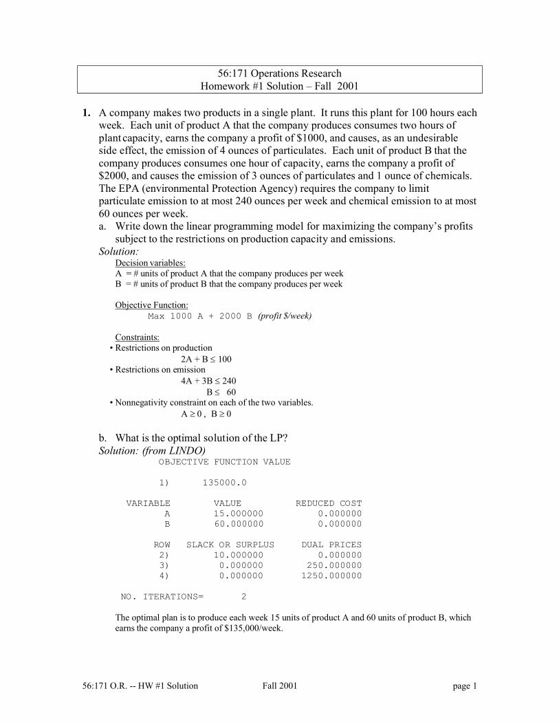
1. A company makes two products in a single plant. It runs this plant for 100 hours eachweek. Each unit of product A that the company produces consumes two hours ofplant capacity, earns the company a profit of $1000, and causes, as an undesirableside effect, the emission of 4 ounces of particulates. Each unit of product B that thecompany produces consumes one hour of capacity, earns the company a profit of$2000, and causes the emission of 3 ounces of particulates and 1 ounce of chemicals. The EPA (environmental Protection Agency) requires the company to limitparticulate emission to at most 240 ounces per week and chemical emission to at most60 ounces per week. a. Write down the linear programming model for maximizing the company’s profits
subject to the restrictions on production capacity and emissions.Solution:
Decision variables:A = # units of product A that the company produces per weekB = # units of product B that the company produces per week
Objective Function: Max 1000 A + 2000 B (profit $/week)
Constraints:• Restrictions on production
2A + B ≤ 100• Restrictions on emission
4A + 3B ≤ 240B ≤ 60
• Nonnegativity constraint on each of the two variables.A ≥ 0 , B ≥ 0
b. What is the optimal solution of the LP?Solution: (from LINDO)
OBJECTIVE FUNCTION VALUE
1) 135000.0
VARIABLE VALUE REDUCED COSTA 15.000000 0.000000B 60.000000 0.000000
ROW SLACK OR SURPLUS DUAL PRICES2) 10.000000 0.0000003) 0.000000 250.0000004) 0.000000 1250.000000
NO. ITERATIONS= 2
The optimal plan is to produce each week 15 units of product A and 60 units of product B, whichearns the company a profit of $135,000/week.

56:171 O.R. -- HW #1 Solution Fall 2001 page 2
2. Cattle feed can be mixed from oats, corn, alfalfa, and peanut hulls. The followingtable shows the current cost per ton (in dollars) of each of these ingredients, togetherwith the percentage of recommended daily allowances for protein, fat, and fiber that aserving of it fulfills.
Oats Corn Alfalfa Peanut hulls% protein 60 80 55 40% fat 50 70 40 100% fiber 90 30 60 80Cost $/ton 200 150 100 75
We want to find a minimum cost way to produce feed that satisfies at least 60% of thedaily allowance for protein and fiber while not exceeding 60% of the fat allowance.
Solution:Decision variables:Define the variables OATS, CORN, ALFALFA, and HULLS to be the quantity (in tons) mixed toobtain a ton of cattle feed.
Complete LP Formulation :
MIN Z = 200 OATS + 150 CORN + 100 ALFALFA + 75 HULLSSUBJECT TO
60 OATS + 80 CORN + 55 ALFALFA + 40 HULLS >= 6050 OATS + 70 CORN + 40 ALFALFA + 100 HULLS <= 6090 OATS + 30 CORN + 60 ALFALFA + 80 HULLS >= 60OATS + CORN + ALFALFA + HULLS = 1OATS >= 0, CORN >= 0, ALFALFA >= 0, HULLS >= 0
Solution from LINDO :
LP OPTIMUM FOUND AT STEP 4
OBJECTIVE FUNCTION VALUE
1) 125.0000
VARIABLE VALUE REDUCED COSTOATS 0.157143 0.000000CORN 0.271429 0.000000
ALFALFA 0.400000 0.000000HULLS 0.171429 0.000000
ROW SLACK OR SURPLUS DUAL PRICES2) 0.000000 -5.0000003) 0.000000 0.0000004) 0.000000 -2.5000005) 0.000000 325.000000
NO. ITERATIONS= 4

56:171 O.R. -- HW #1 Solution Fall 2001 page 3
The optimal solution is to mix 0.16 tons of oats, 0.27 tons of corns, 0.4 tons of alfalfa, and 0.17tons of peanut hulls to obtain a ton of feed. The cost of a ton of feed is $125.
3. “Mama’s Kitchen” serves from 5:30 a.m. each morning until 1:30 p.m. in theafternoon. Tables are set and cleared by busers working 4-hour shifts beginning onthe hour from 5:00 a.m. through 10:00 a.m. Most are college students who hate to getup in the morning, so Mama’s pays $9 per hour for the 5:00, 6:00, and 7:00 a.m.shifts, and $7.50 per hour for the others. (That is, a person works a shift consisting of4 consecutive hours, with the wages equal to 4×$9 for the three early shifts, and4×$7.50 for the 3 later shifts.) The manager seeks a minimum cost staffing plan thatwill have at least the number of busers on duty each hour as specified below:
5 am 6 am 7 am 8 am 9 am 10am 11am Noon 1 pm#reqd 2 3 5 5 3 2 4 6 3Solution:Decision variables:
Xi = the # of employees who start to work on ith shift. ( i = 1, 2, ... , 6 )
LP Formulation :MIN 36 X1 + 36 X2 + 36 X3 + 30 X4 + 30 X5 + 30 X6SUBJECT TOX1 >= 2 (Restriction of # of busers on duty at 5am)X1 + X2 >= 3 (Restriction of # of busers on duty at 6am)X1 + X2 + X3 >= 5 (Restriction of # of busers on duty at 7am)X1 + X2 + X3 + X4 >= 5 (Restriction of # of busers on duty at 8am)
X2 + X3 + X4 + X5 >= 3 (Restriction of # of busers on duty at 9am)X3 + X4 + X5 + X6 >= 2 (Restriction of # of busers on duty at 10am)
X4 + X5 + X6 >= 4 (Restriction of # of busers on duty at 11am)X5 + X6 >= 6 (Restriction of # of busers on duty at 12pm)
X6 >= 3 (Restriction of # of busers on duty at 1pm)Xi >= 0 (for i = 1,2,3,4,5,6) (Sign restrictions)
Solution from LINDO :
LP OPTIMUM FOUND AT STEP 9
OBJECTIVE FUNCTION VALUE1) 360.0000
VARIABLE VALUE REDUCED COSTX1 3.000000 0.000000X3 2.000000 0.000000X5 3.000000 0.000000X6 3.000000 0.000000
ROW SLACK OR SURPLUS DUAL PRICES2) 1.000000 0.0000003) 0.000000 0.0000004) 0.000000 -6.0000005) 0.000000 -30.0000006) 2.000000 0.0000007) 6.000000 0.0000008) 2.000000 0.000000

56:171 O.R. -- HW #1 Solution Fall 2001 page 4
9) 0.000000 -30.00000010) 0.000000 0.000000
That is, the optimal staffing plan is to employ3 busers for the 1st shift(4-hour shifts begins at 5:00a.m.), 2 busers for the 3rd shift(4-hour shifts begins at 7:00a.m.), 3 busers for the 5th shift(4-hour shifts begins at 9:00a.m.), and 3 busers for the 6th shift(4-hour shifts begins at 10:00a.m.).
Note that the solution of the LP (with continuous variables) is actually integer-valued!
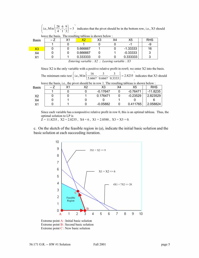
4. a. Draw the feasible region of the following LP:
Maximize 3X1 + 2X2
subject to 4X1 + 7X2 ≤ 28X1 + X2 ≤ 6
3X1 + X2 ≤ 9X1 ≥ 0, X2 ≥ 0
b. Use the simplex algorithm to find the optimal solution of the above LP. (Show theinitial and each succeeding tableau.)
Solution: After adding slack variables X3, X4, and X5 to the three constraints, we obtain theinitial tableau as follows :
Basis – Z X1 X2 X3 X4 X5 RHS1 3 2 0 0 0 0
X3 0 4 7 1 0 0 28X4 0 1 1 0 1 0 6X5 0 3 1 0 0 1 9
Entering variable : X1 ; Leaving variable : X5
Either X1 or X2 might be selected to enter the basis – both have positive relative profits in row 0.Because it has the larger relative profit, we here enter X1 into the basis. The minimum ratio test
FeasibleRegion
3X1 + X2 <= 9
X1 + X2 <= 6
4X1 + 7X2 <= 28
56:171 O.R. -- HW #1 Solution Fall 2001 page 5
28 6 9i.e., Min , , 34 1 3
=
indicates that the pivot should be in the bottom row, i.e., X5 should
leave the basis. The resulting tableau is shown below :Basis – Z X1 X2 X3 X4 X5 RHS
1 0 1 0 0 -1 -9X3 0 0 5.666667 1 0 -1.33333 16X4 0 0 0.666667 0 1 -0.33333 3X1 0 1 0.333333 0 0 0.333333 3
Entering variable : X2 ; Leaving variable : X3
Since X2 is the only variable with a positive relative profit in row0, we enter X2 into the basis.
The minimum ratio test 16 3 3i.e., Min , , 2.82355.6667 0.6667 0.3333
=
indicates that X3 should
leave the basis, i.e., the pivot should be in row 1. The resulting tableau is shown below :Basis – Z X1 X2 X3 X4 X5 RHS
1 0 0 -0.17647 0 -0.76471 -11.8235X2 0 0 1 0.176471 0 -0.23529 2.823529X4 0 1 0 0 1 0 6X1 0 1 0 -0.05882 0 0.411765 2.058824
Since each variable has a nonpositive relative profit in row 0, this is an optimal tableau. Thus, theoptimal solution to LP isZ = 11.8235 , X2 = 2.8235 , X4 = 6 , X1 = 2.0588 , X3 = X5 = 0.
c. On the sketch of the feasible region in (a), indicate the initial basic solution and thebasic solution at each succeeding iteration.
Extreme point A : Initial basic solutionExtreme point B : Second basic solutionExtreme point C : New basic solution
FeasibleRegion
3X1 + X2 <= 9
X1 + X2 <= 6
4X1 + 7X2 <= 28
AB
C

56:171 O.R. -- HW #1 Solution Fall 2001 page 6
5a. What is INFORMS?Institute for Operations Research and theManagement Sciences
5b. Find (on the INFORMS website at http://www.informs.org) a definition of “Operations Research”.
Operations Research (OR) and the Management Sciences (MS) are the professional disciplines thatdeal with the application of information technology for informed decision-making.OR/MS Professionals aim to provide rational bases for decision making by seeking to understand andstructure complex situations and to use this understanding to predict system behavior and improvesystem performance. Much of this work is done using analytical and numerical techniques to developand manipulate mathematical and computer models of organizational systems composed of people,machines, and procedures.
56:171 O.R. HW#2 Solutions Fall 2001 page 1 of 3
56:171 Operations ResearchHomework #2 Solutions -- Fall 2001
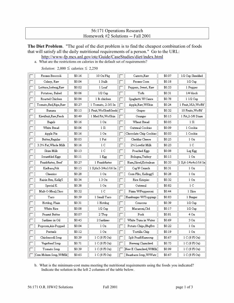
The Diet Problem. "The goal of the diet problem is to find the cheapest combination of foodsthat will satisfy all the daily nutritional requirements of a person." Go to the URL:
http://www-fp.mcs.anl.gov/otc/Guide/CaseStudies/diet/index.htmla. What are the restrictions on calories in the default set of requirements?
Solution: 2,000 ≤ calories ≤ 2,250
b. What is the minimum-cost menu meeting the nutritional requirements using the foods you indicated? Indicate the solution in the left 2 columns of the table below.

56:171 O.R. HW#2 Solutions Fall 2001 page 2 of 3
Change the default upper limit on calories to 1500/day and solve the problem again. (Be sure that the lower bound ≤upper bound!)
c. What is the minimum-cost menu meeting the nutritional requirements using the foods you indicated? Indicate the solution in the right 2 columns of the table below.
Example solution: Note that only six foods are included in the optimal solution! This is a very economical menu,satisfying nutritional requirements, but probably not very satisfying in other ways!
Quantity(# servings) Cost Foods Quantity
(# servings) Cost3.09 0.22 1. Carrots,Raw 3.10 0.2210.00 0.40 2. Celery, Raw 10.00 0.401.44 0.03 3. Lettuce,Iceberg,Raw 2.19 0.04
4. Roasted Chicken5. Spaghetti W/ Sauce6. Wheat Bread7. White Bread8. Chocolate Chip Cookies9. Butter,Regular10. 3.3% Fat,Whole Milk11. 2% Lowfat Milk
2.13 0.28 12. Skim Milk 1.85 0.2413. White Rice
3.18 0.22 14. Peanut Butter 0.15 0.019.95 0.40 15. Popcorn,Air-Popped 8.22 0.33
Total Cost : $1.54/day Total Cost : $1.24/day
* New restrictions on calories : 1,000 ≤ calories ≤ 1,500
2. Below are several simplex tableaus. Assume that the objective in each case is to be minimized. Classify each tableau bywriting to the right of the tableau a letter A through G, according to the descriptions below. Also answer the questionaccompanying each classification, if any.
(A) Nonoptimal, nondegenerate tableau with bounded solution. Circle a pivot element which would improve theobjective.
(B) Nonoptimal, degenerate tableau with bounded solution. Circle an appropriate pivot element. Would theobjective improve with this pivot?
(C) Unique nondegenerate optimum.
(D) Optimal tableau, with alternate optimum. State the values of the basic variables. Circle a pivot element whichwould lead to another optimal basic solution. Which variable will enter the basis, and at what value?
(E) Objective unbounded (below). Specify a variable which, when going to infinity, will make the objectivearbitrarily low.
(F) Tableau with infeasible primal

56:171 O.R. HW#2 Solutions Fall 2001 page 3 of 3
Solution:
56:171 O.R. HW#3 Solution Fall 2001 page 1 of 9
56:171 Operations ResearchHomework #3 Solution, Fall 2001
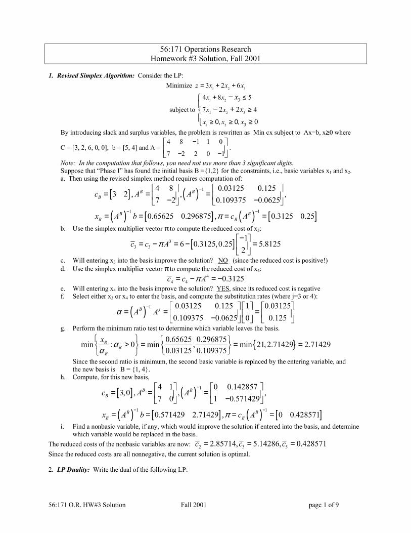
1. Revised Simplex Algorithm: Consider the LP:
1 2 3Minimize 3 2 6z x x x= + +
subject to1 2
2
1 2
3
3
1
3
4 8 5
7 42 2
0
x x
x x
x x x
x
x+ ≤
≥
≥ 0, ≥ 0, ≥
− − +
By introducing slack and surplus variables, the problem is rewritten as Min cx subject to Ax=b, x≥0 where
C = [3, 2, 6, 0, 0], b = [5, 4] and A =4 8 1 1 0
7 2 2 0 1
−
− −
.
Note: In the computation that follows, you need not use more than 3 significant digits.Suppose that “Phase I” has found the initial basis B ={1,2} for the constraints, i.e., basic variables x1 and x2.a. Then using the revised simplex method requires computation of:
[ ] ( )
( ) [ ] ( ) [ ]
1
1 1
4 8 0.03125 0.1253 2 , , ,
7 2 0.109375 0.0625
0.65625 0.296875 , 0.3125 0.25
B BB
B BB B
c A A
x A b c Aπ
−
− −
= = = − −
= = = =b. Use the simplex multiplier vector π to compute the reduced cost of x3:
[ ]33 3
16 0.3125,0.25 5.8125
2c c Aπ
− = − = − =
c. Will entering x3 into the basis improve the solution? _NO_ (since the reduced cost is positive!)d. Use the simplex multiplier vector π to compute the reduced cost of x4:
44 4 0.3125c c Aπ= − = −
e. Will entering x4 into the basis improve the solution? YES, since its reduced cost is negativef. Select either x3 or x4 to enter the basis, and compute the substitution rates (where j=3 or 4):
( ) 1 0.03125 0.125 1 0.031250.109375 0.0625 0 0.125
B jA Aα−
= = = − g. Perform the minimum ratio test to determine which variable leaves the basis.
{ }0.65625 0.296875min : 0 min , min 21, 2.71429 2.714290.03125 0.109375
BB
B
x αα > = = =
Since the second ratio is minimum, the second basic variable is replaced by the entering variable, andthe new basis is B = {1, 4}.
h. Compute, for this new basis,
[ ] ( )
( ) [ ] ( ) [ ]
1
1 1
4 1 0 0.1428573,0 , , ,
7 0 1 0.571429
0.571429 2.71429 , 0 0.428571
B BB
B BB B
c A A
x A b c Aπ
−
− −
= = = −
= = = =i. Find a nonbasic variable, if any, which would improve the solution if entered into the basis, and determine
which variable would be replaced in the basis.The reduced costs of the nonbasic variables are now: 2 3 52.85714, 5.14286, 0.428571c c c= = =Since the reduced costs are all nonnegative, the current solution is optimal.
2. LP Duality: Write the dual of the following LP:

56:171 O.R. HW#3 Solution Fall 2001 page 2 of 9
1 2 33 2 4Min x x x+ −
subject to
1 2 3
1 2 3
1 3
2 3
5 72 18
2 62
, j=1,2,3j
x x xx x x
x xx xx
− + ≥12 − + = − ≤ + ≥10 ≥ 0
Solution:
1 2 3 412 18 6 10Maximize y y y y+ + +subject to
1 2 3
1 2 4
1 2 3 4
5 37 22 2 4
y y yy y y
y y y y
+ + ≤ − − + ≤ + − + ≤ −
with sign restrictions: y1≥0, y3≤0,y4≥0 (y2 unrestricted in sign)
3. Consider the following primal LP problem:
1 2 3 4 52 9 8 36Max x x x x x+ − + −
subject to2 3 4 5
1 2 4 5
2 3 402 2 10
0, j=1,2,3,4,5j
x x x xx x x xx
− + − ≤ − + − ≤ ≥
a. Write the dual LP problemSolution:
1 240 10Min y y+subject to:
2
1 2
1
1 2
1 2
12 2
92 8
3 2 36
yy y
yy yy y
≥ − ≥ − ≥ − + ≥− − ≥ −
and yj ≥ 0, j=1,2b. Sketch the feasible region of the dual LP in 2 dimensions, and use it to find the optimal solution.

56:171 O.R. HW#3 Solution Fall 2001 page 3 of 9
The objective function evaluated at the points A(2.4, 2.8), B(4.667, 7.333), C(9, 4.5), D(9, 1), and E(3.5, 1) are124, 260, 405, 370, and 150, respectively, so that the minimum value(=124) is achieved at (2.4, 2.8), i.e.,y1=2.4, y2=2.8.c. Using complementary slackness conditions,
♦ write equations which must be satisfied by the optimal primal solution x*Solution: Since both y1 , y2 are positive, primal constraint (1) and (2) must be tight, i.e.,
2 3 4 52 3 40x x x x− + − = , 1 2 4 52 2 10x x x x− + − = .♦ which primal variables must be zero?Solution: since constraints (1), (3), and (5) are slack, the primal variables x1, x3, and x5 must be zero.
d. Using the information in (c.), determine the optimal solution x*.Solution: x2 = 14 & x4 = 12 , while xj = 0 for j=1, 3, 5. e. Compare the optimal objective values of the primal and dual solutions.Solution: at x*, the objective function is 2×14 + 8×12=124, which is identical to the optimal dual objective value.
4. LP Sensitivity Analysis: Cornco produces two products: PS and QT. The sales price for each product and themaximum quantity of each that can be sold during each of the next three months are:
Month 1 Month 2 Month 3Product Price Demand Price Demand Price Demand
PS $40 50 $60 45 $55 50QT $35 43 $40 50 $44 40
Each product must be processed through two assembly lines: 1 & 2. The number of hours required by each producton each assembly line are:
Product Line 1 Line 2PS 3 hours 2 hoursQT 2 hours 2 hours

56:171 O.R. HW#3 Solution Fall 2001 page 4 of 9
The number of hours available on each assembly line during each month are:Line Month 1 Month 2 Month 3
1 200 160 1902 140 150 110
Each unit of PS requires 4 pounds of raw material while each unit of QT requires 3 pounds. A total of 710 units ofraw material can be purchased during the three-month interval at $3 per pound. At the beginning of month 1, 10units of PS and 5 units of QT are available. It costs $10 to hold a unit of a unit of either product in inventory for amonth.
Solution:Define variablesPt = # units of product PS produced in month t, t=1,2,3Qt = # units of product QT produced in month t, t=1,2,3R = (total) # units of raw material purchasedSt = # units of product PS sold in month t, t=1,2,3Tt = # units of product QT sold in month t, t=1,2,3It = # units of product PS in inventory at end of month t, t=0,1,2Jt = # units of product QT in inventory at end of month t, t=0,1,2Objective: Maximize profit =
40S1 + 60S2 + 55S3 (revenue from sale of PS)+35T1 + 40T2 + 44T3 (revenue from sale of QT)- 3R (purchase of raw material)- 10I1 - 10I2 (storage cost of PS)- 10J1 - 10 J2 (storage cost of QT)
Subject to the constraints:R ≤ 710 (limited availability of raw material)S1 ≤ 50, S2 ≤ 45, S3 ≤ 50 (demand constraints for PS)T1 ≤ 43, T2 ≤ 50, T3 ≤ 40 (demand constraints for QT)3P1 +2Q1 ≤ 200 (hours available on line 1, month 1)3P2 +2Q2 ≤ 160 (hours available on line 1, month 2)3P3 +2Q3 ≤ 190 (hours available on line 1, month 3)2P1 +2Q1 ≤ 140 (hours available on line 2, month 1)2P2 +2Q2 ≤ 150 (hours available on line 2, month 2)2P3 +2Q3 ≤ 110 (hours available on line 2, month 3)P1 + I0 = 50 + S1+I1 (material balance of PS, month 1)P2 + I1 = 45 + S2+I2 (material balance of PS, month 2)P3 + I2 = 50 + S3 (material balance of PS, month 3)Q1 + J0 = 43 + T1+J1 (material balance of QT, month 1)Q2 + J1 = 50 + T2+J2 (material balance of QT, month 2)Q3 + J2 = 40 + T3 (material balance of QT, month 3)4P1+3Q1+4P2+3Q2+4P3+3Q3 ≤ R (consumption of raw material)
Note: the upper bounds on R, St, Tt, etc. could be imposed either by using the "simple upper bound" (SUB)command or by adding a row to the problem. The former is preferred!
LINDO output:
MAX 40 S1 + 60 S2 + 55 S3 + 35 T1 + 40 T2 + 44 T3 - 3 R - 10 I1- 10 I2 - 10 J1 - 10 J2
SUBJECT TO2) 3 P1 + 2 Q1 <= 2003) 3 P2 + 2 Q2 <= 1604) 3 P3 + 2 Q3 <= 1905) 2 P1 + 2 Q1 <= 1406) 2 P2 + 2 Q2 <= 1507) 2 P3 + 2 Q3 <= 1108) - S1 - I1 + P1 + I0 = 09) - S2 + I1 - I2 + P2 = 010) - S3 + I2 + P3 = 0
56:171 O.R. HW#3 Solution Fall 2001 page 5 of 9
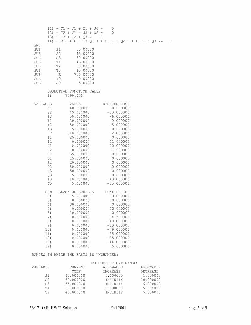
11) - T1 - J1 + Q1 + J0 = 012) - T2 + J1 - J2 + Q2 = 013) - T3 + J2 + Q3 = 014) - R + 4 P1 + 3 Q1 + 4 P2 + 3 Q2 + 4 P3 + 3 Q3 <= 0
ENDSUB S1 50.00000SUB S2 45.00000SUB S3 50.00000SUB T1 43.00000SUB T2 50.00000SUB T3 40.00000SUB R 710.00000SUB I0 10.00000SUB J0 5.00000
OBJECTIVE FUNCTION VALUE1) 7590.000
VARIABLE VALUE REDUCED COSTS1 40.000000 0.000000S2 45.000000 -10.000000S3 50.000000 -6.000000T1 20.000000 0.000000T2 50.000000 -5.000000T3 5.000000 0.000000R 710.000000 -2.000000I1 25.000000 0.000000I2 0.000000 11.000000J1 0.000000 10.000000J2 0.000000 1.000000P1 55.000000 0.000000Q1 15.000000 0.000000P2 20.000000 0.000000Q2 50.000000 0.000000P3 50.000000 0.000000Q3 5.000000 0.000000I0 10.000000 -40.000000J0 5.000000 -35.000000
ROW SLACK OR SURPLUS DUAL PRICES2) 5.000000 0.0000003) 0.000000 10.0000004) 30.000000 0.0000005) 0.000000 10.0000006) 10.000000 0.0000007) 0.000000 14.5000008) 0.000000 -40.0000009) 0.000000 -50.000000
10) 0.000000 -49.00000011) 0.000000 -35.00000012) 0.000000 -35.00000013) 0.000000 -44.00000014) 0.000000 5.000000
RANGES IN WHICH THE BASIS IS UNCHANGED:
OBJ COEFFICIENT RANGESVARIABLE CURRENT ALLOWABLE ALLOWABLE
COEF INCREASE DECREASES1 40.000000 5.000000 1.000000S2 60.000000 INFINITY 10.000000S3 55.000000 INFINITY 6.000000T1 35.000000 2.000000 5.000000T2 40.000000 INFINITY 5.000000

56:171 O.R. HW#3 Solution Fall 2001 page 6 of 9
T3 44.000000 1.000000 29.000000R -3.000000 INFINITY 2.000000
I1 -10.000000 1.500000 7.500000I2 -10.000000 11.000000 INFINITYJ1 -10.000000 10.000000 INFINITYJ2 -10.000000 1.000000 INFINITYP1 0.000000 6.000000 2.000000Q1 0.000000 2.000000 5.000000P2 0.000000 7.500000 1.500000Q2 0.000000 1.000000 5.000000P3 0.000000 INFINITY 6.000000Q3 0.000000 6.000000 29.000000I0 0.000000 INFINITY 40.000000J0 0.000000 INFINITY 35.000000
RIGHTHAND SIDE RANGESROW CURRENT ALLOWABLE ALLOWABLE
RHS INCREASE DECREASE2 200.000000 INFINITY 5.0000003 160.000000 15.000000 3.7500004 190.000000 INFINITY 30.0000005 140.000000 11.500000 6.6666676 150.000000 INFINITY 10.0000007 110.000000 15.333333 3.3333338 0.000000 40.000000 10.0000009 0.000000 40.000000 10.000000
10 0.000000 5.000000 5.00000011 0.000000 20.000000 23.00000012 0.000000 15.000000 10.00000013 0.000000 5.000000 35.00000014 0.000000 5.000000 23.000000
THE TABLEAU
ROW (BASIS) S1 S2 S3 T1 T2 T31 ART 0.000 10.000 6.000 0.000 5.000 0.0002 SLK 2 0.000 0.000 1.000 0.000 0.333 0.0003 Q2 0.000 0.000 0.000 0.000 1.000 0.0004 SLK 4 0.000 0.000 -1.000 0.000 0.000 0.0005 S1 1.000 -1.000 -1.000 0.000 -1.000 0.0006 SLK 6 0.000 0.000 0.000 0.000 -0.667 0.0007 Q3 0.000 0.000 -1.000 0.000 0.000 0.0008 I1 0.000 1.000 0.000 0.000 0.667 0.0009 T1 0.000 0.000 1.000 1.000 0.333 0.000
10 P3 0.000 0.000 1.000 0.000 0.000 0.00011 Q1 0.000 0.000 1.000 0.000 0.333 0.00012 P1 0.000 0.000 -1.000 0.000 -0.333 0.00013 T3 0.000 0.000 -1.000 0.000 0.000 1.00014 P2 0.000 0.000 0.000 0.000 -0.667 0.000
ROW R I1 I2 J1 J2 P1 Q11 2.000 0.000 11.000 10.000 1.000 0.000 0.0002 -1.000 0.000 1.000 0.333 -0.333 0.000 0.0003 0.000 0.000 0.000 1.000 -1.000 0.000 0.0004 0.000 0.000 -1.000 0.000 0.000 0.000 0.0005 1.000 0.000 0.000 -1.000 1.000 0.000 0.0006 0.000 0.000 0.000 -0.667 0.667 0.000 0.0007 0.000 0.000 -1.000 0.000 0.000 0.000 0.0008 0.000 1.000 -1.000 0.667 -0.667 0.000 0.0009 -1.000 0.000 1.000 1.333 -0.333 0.000 0.000
10 0.000 0.000 1.000 0.000 0.000 0.000 0.00011 -1.000 0.000 1.000 0.333 -0.333 0.000 1.00012 1.000 0.000 -1.000 -0.333 0.333 1.000 0.00013 0.000 0.000 -1.000 0.000 -1.000 0.000 0.000

56:171 O.R. HW#3 Solution Fall 2001 page 7 of 9
14 0.000 0.000 0.000 -0.667 0.667 0.000 0.000
ROW P2 Q2 P3 Q3 I0 J0 SLK 21 0.000 0.000 0.000 0.000 40.000 35.000 0.0002 0.000 0.000 0.000 0.000 0.000 0.000 1.0003 0.000 1.000 0.000 0.000 0.000 0.000 0.0004 0.000 0.000 0.000 0.000 0.000 0.000 0.0005 0.000 0.000 0.000 0.000 1.000 0.000 0.0006 0.000 0.000 0.000 0.000 0.000 0.000 0.0007 0.000 0.000 0.000 1.000 0.000 0.000 0.0008 0.000 0.000 0.000 0.000 0.000 0.000 0.0009 0.000 0.000 0.000 0.000 0.000 1.000 0.000
10 0.000 0.000 1.000 0.000 0.000 0.000 0.00011 0.000 0.000 0.000 0.000 0.000 0.000 0.00012 0.000 0.000 0.000 0.000 0.000 0.000 0.00013 0.000 0.000 0.000 0.000 0.000 0.000 0.00014 1.000 0.000 0.000 0.000 0.000 0.000 0.000
ROW SLK 3 SLK 4 SLK 5 SLK 6 SLK 7 SLK 141 10.000 0.000 10.000 0.000 14.500 5.000 7590.0002 1.333 0.000 0.500 0.000 1.500 -1.000 5.0003 0.000 0.000 0.000 0.000 0.000 0.000 50.0004 0.000 1.000 0.000 0.000 -1.000 0.000 30.0005 -1.000 0.000 -1.500 0.000 -1.500 1.000 40.0006 -0.667 0.000 0.000 1.000 0.000 0.000 10.0007 0.000 0.000 0.000 0.000 0.500 0.000 5.0008 -0.333 0.000 0.000 0.000 0.000 0.000 25.0009 1.333 0.000 2.000 0.000 1.500 -1.000 20.000
10 0.000 0.000 0.000 0.000 0.000 0.000 50.00011 1.333 0.000 2.000 0.000 1.500 -1.000 15.00012 -1.333 0.000 -1.500 0.000 -1.500 1.000 55.00013 0.000 0.000 0.000 0.000 0.500 0.000 5.00014 0.333 0.000 0.000 0.000 0.000 0.000 20.00016 0.500 0.000 0.000 0.000 5.000
Answer the questions below, using the output above for the original problem, if possible. If not possible, youneed not run LINDO again.
a. Find the new optimal solution if it costs $11 to hold a unit of PS in inventory at the end of month 1.
Solution: The current objective coefficient of I1 (the amount of PS in inventory at the end of month 1) is −10. OBJ COEFFICIENT RANGES
VARIABLE CURRENT ALLOWABLE ALLOWABLECOEF INCREASE DECREASE
I1 -10.000000 1.500000 7.500000
According to the above LINDO output, the current basis is optimal for values of this coefficient between−10−7.5=−17.5and −10+11=+1. If the inventory cost were $11, the new coefficient would be −11, which iswithin the range [−17.5, +1], so the current basis remains optimal and the values of the basic variables areunchanged.
b. Find the company's new optimal solution if 210 hours on line 1 are available during month 1.
Solution: Currently 200 hours (the right-hand-side of row 2) are available on line 1 in month 1, of which 195 areused (since the slack in this constraint is 5). The range within which the current basis remains optimal is200−5to 200+∞, i.e., the range [195, +∞]. Since 210 is within this range, the current basis remains optimal,although the value of the basic variable SLK2 will increase from 5 to 15.
RIGHTHAND SIDE RANGESROW CURRENT ALLOWABLE ALLOWABLE
RHS INCREASE DECREASE2 200.000000 INFINITY 5.000000
c. Find the company's new profit level if 109 hours are available on line 2 during month 3.
Solution: The right-hand-side of row 7 would be changed: 7) 2 P3 + 2 Q3 <= 110
56:171 O.R. HW#3 Solution Fall 2001 page 8 of 9
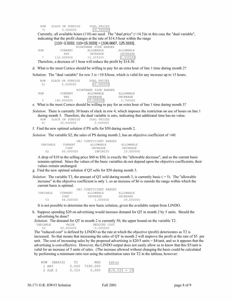
ROW SLACK OR SURPLUS DUAL PRICES7) 0.000000 14.500000
Currently, all available hours (110) are used. The "dual price" (+14.5)is in this case the "dual variable",indicating that the profit changes at the rate of $14.5/hour within the range
[110−3.3333, 110+15.3333] = [106.6667, 125.3333]. RIGHTHAND SIDE RANGES
ROW CURRENT ALLOWABLE ALLOWABLERHS INCREASE DECREASE
7 110.000000 15.333333 3.333333
Therefore, a decrease of 1 hour will reduce the profit by $14.50.
d. What is the most Cornco should be willing to pay for an extra hour of line 1 time during month 2?
Solution: The "dual variable" for row 3 is +10 $/hour, which is valid for any increase up to 15 hours.ROW SLACK OR SURPLUS DUAL PRICES3) 0.000000 10.000000
RIGHTHAND SIDE RANGESROW CURRENT ALLOWABLE ALLOWABLE
RHS INCREASE DECREASE3 160.000000 15.000000 3.750000
e. What is the most Cornco should be willing to pay for an extra hour of line 1 time during month 3?
Solution: There is currently 30 hours of slack in row 4, which imposes the restriction on use of hours on line 1during month 3. Therefore, the dual variable is zero, indicating that additional time has no value.ROW SLACK OR SURPLUS DUAL PRICES4) 30.000000 0.000000
f. Find the new optimal solution if PS sells for $50 during month 2.
Solution: The variable S2, the sales of PS during month 2, has an objective coefficient of +60:OBJ COEFFICIENT RANGES
VARIABLE CURRENT ALLOWABLE ALLOWABLECOEF INCREASE DECREASE
S2 60.000000 INFINITY 10.000000
A drop of $10 in the selling price $60 to $50, is exactly the "allowable decrease", and so the current basisremains optimal. Since the values of the basic variables do not depend upon the objective coefficients, theirvalues remain unchanged.
g. Find the new optimal solution if QT sells for $50 during month 3.
Solution: The variable T3, the amount of QT sold during month 3, is currently basic ( = 5). The "allowableincrease" in the objective coefficient is only 1, so an increase of $6 is outside the range within which thecurrent basis is optimal.
OBJ COEFFICIENT RANGESVARIABLE CURRENT ALLOWABLE ALLOWABLE
COEF INCREASE DECREASET3 44.000000 1.000000 29.000000
It is not possible to determine the new basic solution, given the available output from LINDO.
h. Suppose spending $20 on advertising would increase demand for QT in month 2 by 5 units. Should theadvertising be done?
Solution: The demand for QT in month 2 is currently 50, the upper bound on the variable T2. VARIABLE VALUE REDUCED COST
T2 50.000000 -5.000000
The "reduced cost" is defined by LINDO as the rate at which the objective (profit) deteriorates as T2 isincreased. So that means that increasing the sales of QT in month 2 will improve the profit at the rate of $5 perunit. The cost of increasing sales by the proposed advertising is $20/5 units = $4/unit, and so it appears that theadvertising is cost-effective. However, the LINDO output does not easily allow us to know that this $5/unit isvalid for an increase of 5 units of sales. (The increase allowed without changing the basis could be calculatedby performing a minimum ratio test using the substitution rates for T2 in the tableau, however:
ROW (BASIS) T2 RHS ratio1 ART 5.000 7590.0002 SLK 2 0.333 5.000 5/0.333 = 15

56:171 O.R. HW#3 Solution Fall 2001 page 9 of 9
3 Q2 1.000 50.000 50/1 = 504 SLK 4 0.000 30.0005 S1 -1.000 40.0006 SLK 6 -0.667 10.0007 Q3 0.000 5.0008 I1 0.667 25.000 25/0.667 = 37.59 T1 0.333 20.000 20/0.333 = 60
10 P3 0.000 50.00011 Q1 0.333 15.000 15/0.333 = 4512 P1 -0.333 55.00013 T3 0.000 5.00014 P2 -0.667 20.000
This calculation indicates that an increase of 15 units in T2 is allowed before a basic variable (SLK 2) isreduced to zero, preventing any further increase of T2.

56:171 O.R. HW#4 Solutions Fall 2001 page 1 of 9
56:171 Operations ResearchHomework #4 Solutions -- Fall 2001
1. Linear Programming sensitivity. A paper recycling plant processes box board, tissue paper, newsprint, andbook paper into pulp that can be used to produce three grades of recycled paper (grades 1, 2, and 3). The pricesper ton and the pulp contents of the four inputs are:
Input Cost Pulptype $/ton content
Box board 5 15%Tissue paper 6 20%Newsprint 8 30%Book paper 10 40%
Two methods, de-inking and asphalt dispersion, can be used to process the four inputs into pulp. It costs $20 tode-ink a ton of any input. The process of de-inking removes 10% of the input's pulp. It costs $15 to applyasphalt dispersion to a ton of material. The asphalt dispersion process removes 20% of the input's pulp. Atmost 3000 tons of input can be run through the asphalt dispersion process or the de-inking process. Grade 1paper can only be produced with newsprint or book paper pulp; grade 2 paper, only with book paper, tissuepaper, or box board pulp; and grade 3 paper, only with newsprint, tissue paper, or box board pulp. To meet itscurrent demands, the company needs 500 tons of pulp for grade 1 paper, 500 tons of pulp for grade 2 paper,and 600 tons of pulp for grade 3 paper. The LP model below was formulated to minimize the cost of meetingthe demands for pulp.
Define the variablesBOX = tons of purchased boxboardTISS = tons of purchased tissueNEWS = tons of purchased newsprintBOOK = tons of purchased book paperBOX1 = tons of boxboard sent through de-inkingTISS1 = tons of tissue sent through de-inkingNEWS1 = tons of newsprint sent through de-inkingBOOK1 = tons of book paper sent through de-inkingBOX2 = tons of boxboard sent through asphalt dispersionTISS2 = tons of tissue sent through asphalt dispersionNEWS2 = tons of newsprint sent through asphalt dispersionBOOK2 = tons of book paper sent through asphalt dispersionPBOX = tons of pulp recovered from boxboardPTISS = tons of pulp recovered from tissuePNEWS= tons of pulp recovered from newsprintPBOOK = tons of pulp recovered from book paperPBOX1 = tons of boxboard pulp used for grade 1 paper,PBOX2 = tons of boxboard pulp used for grade 2 paper, etc....PBOOK3 = tons of book paper pulp used for grade 3 paper.
The LP model using these variables is:MIN 5 BOX +6 TISS +8 NEWS +10 BOOK +20 BOX1 +20 TISS1 +20 NEWS1
+20 BOOK1 +15 BOX2 +15 TISS2 +15 NEWS2 +15 BOOK2SUBJECT TO
2) - BOX + BOX1 + BOX2 <= 0 3) - TISS + TISS1 + TISS2 <= 0 4) - NEWS + NEWS1 + NEWS2 <= 0 5) - BOOK + BOOK1 + BOOK2 <= 0 6) 0.135 BOX1 + 0.12 BOX2 - PBOX = 07) 0.18 TISS1 + 0.16 TISS2 - PTISS = 08) 0.27 NEWS1 + 0.24 NEWS2 - PNEWS = 09) 0.36 BOOK1 + 0.32 BOOK2 - PBOOK = 010) - PBOX + PBOX2 + PBOX3 <= 011) - PTISS + PTISS2 + PTISS3 <= 012) - PNEWS + PNEWS1 + PNEWS3 <= 013) - PBOOK + PBOOK1 + PBOOK2 <= 014) PNEWS1 + PBOOK1 >= 50015) PBOX2 + PTISS2 + PBOOK2 >= 500

56:171 O.R. HW#4 Solutions Fall 2001 page 2 of 9
16) PBOX3 + PTISS3 + PNEWS3 >= 60017) BOX1 + TISS1 + NEWS1 + BOOK1 <= 300018) BOX2 + TISS2 + NEWS2 + BOOK2 <= 3000
END• Rows 2-5 state that only the supply of each input material which is purchased can be processed, either by
de-inking or asphalt dispersion.• Row 6 states that the recovered pulp in the boxboard is 90% of that in the boxboard which is processed
by de-inking, i.e., (0.90)(0.15)BOX1, since boxboard is 15% pulp, plus 80% of that in the boxboardwhich is processed by asphalt dispersion, i.e., (0.80)(0.15)BOX2.
• Rows 7-9 are similar to row 6, but for different input materials.• Rows 10-13 state that no more than the pulp which is recovered from each input may be used in making
paper (grades 1, 2, &/or 3). Note that some variables are omitted, e.g., PBOX1, since boxboard cannotbe used in Grade 1 paper.
• Rows 14-16 state that the demand for each grade of paper must be satisfied.• Rows 17-18 state that each process (de-inking & asphalt dispersion) has a maximum throughput of 3000
tons. (The problem statement is unclear here, and might be interpreted as stating the total throughput ofboth processes cannot exceed 3000 tons, in which case rows 17&18 would be replaced by17) BOX1 + TISS1 + NEWS1 + BOOK1
+ BOX2 + TISS2 + NEWS2 + BOOK2 <= 3000The solution found by LINDO is as follows:
LP OPTIMUM FOUND AT STEP 25OBJECTIVE FUNCTION VALUE
1) 140000.0
VARIABLE VALUE REDUCED COSTBOX 0.000000 0.000000
TISS 0.000000 6.000000NEWS 2500.000000 0.000000BOOK 2833.333252 0.000000BOX1 0.000000 11.124999TISS1 0.000000 1.499999NEWS1 0.000000 0.249999BOOK1 2333.333252 0.000000BOX2 0.000000 9.333334TISS2 0.000000 0.222223NEWS2 2500.000000 0.000000BOOK2 500.000000 0.000000PBOX 0.000000 0.000000PTISS 0.000000 0.000000PNEWS 600.000000 0.000000PBOOK 1000.000000 0.000000PBOX2 0.000000 19.444445PBOX3 0.000000 0.000000
PTISS2 0.000000 19.444445PTISS3 0.000000 0.000000PNEWS1 0.000000 19.444445PNEWS3 600.000000 0.000000PBOOK1 500.000000 0.000000PBOOK2 500.000000 0.000000
ROW SLACK OR SURPLUS DUAL PRICES2) 0.000000 5.0000003) 0.000000 0.0000004) 0.000000 8.0000005) 0.000000 10.0000006) 0.000000 -102.7777797) 0.000000 -102.7777798) 0.000000 -102.7777799) 0.000000 -83.33333610) 0.000000 102.77777911) 0.000000 102.77777912) 0.000000 102.77777913) 0.000000 83.33333614) 0.000000 -83.33333615) 0.000000 -83.333336

56:171 O.R. HW#4 Solutions Fall 2001 page 3 of 9
16) 0.000000 -102.77777917) 666.666687 0.00000018) 0.000000 1.666667
RANGES IN WHICH THE BASIS IS UNCHANGED:OBJ COEFFICIENT RANGES
VARIABLE CURRENT ALLOWABLE ALLOWABLECOEF INCREASE DECREASE
BOX 5.000000 INFINITY 5.000000TISS 6.000000 INFINITY 6.000000NEWS 8.000000 0.333334 4.666667BOOK 10.000000 6.000000 1.999989BOX1 20.000000 INFINITY 11.124999
TISS1 20.000000 INFINITY 1.499999NEWS1 20.000000 INFINITY 0.249999BOOK1 20.000000 0.249999 0.750001BOX2 15.000000 INFINITY 9.333333
TISS2 15.000000 INFINITY 0.222222NEWS2 15.000000 0.222221 4.666667BOOK2 15.000000 0.666667 0.222221PBOX 0.000000 INFINITY 77.777779
PTISS 0.000000 INFINITY 1.388890PNEWS 0.000000 1.388890 19.444443PBOOK 0.000000 19.444443 83.333336PBOX2 0.000000 INFINITY 19.444443PBOX3 0.000000 19.444443 77.777779PTISS2 0.000000 INFINITY 19.444443PTISS3 0.000000 19.444443 1.388890PNEWS1 0.000000 INFINITY 19.444443PNEWS3 0.000000 1.388890 19.444443PBOOK1 0.000000 19.444443 83.333336PBOOK2 0.000000 19.444443 83.333336
RIGHTHAND SIDE RANGESROW CURRENT ALLOWABLE ALLOWABLE
RHS INCREASE DECREASE2 0.000000 0.000000 INFINITY3 0.000000 INFINITY 0.0000004 0.000000 2500.000000 INFINITY5 0.000000 2833.333252 INFINITY6 0.000000 0.000000 600.0000007 0.000000 0.000000 600.0000008 0.000000 120.000008 600.0000009 0.000000 240.000015 840.00000010 0.000000 600.000000 0.00000011 0.000000 600.000000 0.00000012 0.000000 600.000000 120.00000813 0.000000 840.000000 240.00001514 500.000000 240.000015 500.00000015 500.000000 240.000015 500.00000016 600.000000 120.000008 600.00000017 3000.000000 INFINITY 666.66668718 3000.000000 2625.000000 500.000000
THE TABLEAU
ROW (BASIS) BOX TISS NEWS BOOK BOX1 TISS11 ART 0.000 6.000 0.000 0.000 11.125 1.5002 BOOK 0.000 0.000 0.000 1.000 -0.062 -0.0833 SLK 3 0.000 -1.000 0.000 0.000 0.000 1.0004 SLK 17 0.000 0.000 0.000 0.000 0.500 0.3335 BOOK1 0.000 0.000 0.000 0.000 0.500 0.6676 PBOX 0.000 0.000 0.000 0.000 -0.135 0.0007 PTISS 0.000 0.000 0.000 0.000 0.000 -0.1808 PNEWS 0.000 0.000 0.000 0.000 0.135 0.1809 PBOOK 0.000 0.000 0.000 0.000 0.000 0.00010 PBOX3 0.000 0.000 0.000 0.000 -0.135 0.00011 PTISS3 0.000 0.000 0.000 0.000 0.000 -0.18012 PNEWS3 0.000 0.000 0.000 0.000 0.135 0.180

56:171 O.R. HW#4 Solutions Fall 2001 page 4 of 9
13 PBOOK2 0.000 0.000 0.000 0.000 0.000 0.00014 PBOOK1 0.000 0.000 0.000 0.000 0.000 0.00015 NEWS2 0.000 0.000 0.000 0.000 0.562 0.75016 NEWS 0.000 0.000 1.000 0.000 0.562 0.75017 BOX 1.000 0.000 0.000 0.000 -1.000 0.00018 BOOK2 0.000 0.000 0.000 0.000 -0.562 -0.750
ROW NEWS1 BOOK1 BOX2 TISS2 NEWS2 BOOK2 PBOX1 0.250 0.000 9.333 0.222 0.000 0.000 0.0002 -0.125 0.000 0.056 0.037 0.000 0.000 0.0003 0.000 0.000 0.000 1.000 0.000 0.000 0.0004 0.000 0.000 0.444 0.296 0.000 0.000 0.0005 1.000 1.000 -0.444 -0.296 0.000 0.000 0.0006 0.000 0.000 -0.120 0.000 0.000 0.000 1.0007 0.000 0.000 0.000 -0.160 0.000 0.000 0.0008 0.000 0.000 0.120 0.160 0.000 0.000 0.0009 0.000 0.000 0.000 0.000 0.000 0.000 0.00010 0.000 0.000 -0.120 0.000 0.000 0.000 0.00011 0.000 0.000 0.000 -0.160 0.000 0.000 0.00012 0.000 0.000 0.120 0.160 0.000 0.000 0.00013 0.000 0.000 0.000 0.000 0.000 0.000 0.00014 0.000 0.000 0.000 0.000 0.000 0.000 0.00015 1.125 0.000 0.500 0.667 1.000 0.000 0.00016 0.125 0.000 0.500 0.667 0.000 0.000 0.00017 0.000 0.000 -1.000 0.000 0.000 0.000 0.00018 -1.125 0.000 0.500 0.333 0.000 1.000 0.000
ROW PTISS PNEWS PBOOK PBOX2 PBOX3 PTISS2 PTISS31 0.000 0.000 0.000 19.444 0.000 19.444 0.0002 0.000 0.000 0.000 3.241 0.000 3.241 0.0003 0.000 0.000 0.000 0.000 0.000 0.000 0.0004 0.000 0.000 0.000 0.926 0.000 0.926 0.0005 0.000 0.000 0.000 -0.926 0.000 -0.926 0.0006 0.000 0.000 0.000 0.000 0.000 0.000 0.0007 1.000 0.000 0.000 0.000 0.000 0.000 0.0008 0.000 1.000 0.000 -1.000 0.000 -1.000 0.0009 0.000 0.000 1.000 1.000 0.000 1.000 0.00010 0.000 0.000 0.000 1.000 1.000 0.000 0.00011 0.000 0.000 0.000 0.000 0.000 1.000 1.00012 0.000 0.000 0.000 -1.000 0.000 -1.000 0.00013 0.000 0.000 0.000 1.000 0.000 1.000 0.00014 0.000 0.000 0.000 0.000 0.000 0.000 0.00015 0.000 0.000 0.000 -4.167 0.000 -4.167 0.00016 0.000 0.000 0.000 -4.167 0.000 -4.167 0.00017 0.000 0.000 0.000 0.000 0.000 0.000 0.00018 0.000 0.000 0.000 4.167 0.000 4.167 0.000
ROW PNEWS1 PNEWS3 PBOOK1 PBOOK2 SLK 2 SLK 3 SLK 41 19.444 0.000 0.000 0.000 5.000 0.000 8.0002 3.241 0.000 0.000 0.000 0.000 0.000 0.0003 0.000 0.000 0.000 0.000 0.000 1.000 0.0004 0.926 0.000 0.000 0.000 0.000 0.000 0.0005 -0.926 0.000 0.000 0.000 0.000 0.000 0.0006 0.000 0.000 0.000 0.000 0.000 0.000 0.0007 0.000 0.000 0.000 0.000 0.000 0.000 0.0008 -1.000 0.000 0.000 0.000 0.000 0.000 0.0009 1.000 0.000 0.000 0.000 0.000 0.000 0.00010 0.000 0.000 0.000 0.000 0.000 0.000 0.00011 0.000 0.000 0.000 0.000 0.000 0.000 0.00012 0.000 1.000 0.000 0.000 0.000 0.000 0.00013 0.000 0.000 0.000 1.000 0.000 0.000 0.00014 1.000 0.000 1.000 0.000 0.000 0.000 0.00015 -4.167 0.000 0.000 0.000 0.000 0.000 0.00016 -4.167 0.000 0.000 0.000 0.000 0.000 -1.00017 0.000 0.000 0.000 0.000 -1.000 0.000 0.00018 4.167 0.000 0.000 0.000 0.000 0.000 0.000
ROW SLK 5 SLK 10 SLK 11 SLK 12 SLK 13 SLK 14 SLK 151 10.000 102.778 102.778 102.778 83.333 83.333 83.333

56:171 O.R. HW#4 Solutions Fall 2001 page 5 of 9
2 -1.000 0.463 0.463 0.463 -2.778 -2.778 -2.7783 0.000 0.000 0.000 0.000 0.000 0.000 0.0004 0.000 3.704 3.704 3.704 2.778 2.778 2.7785 0.000 -3.704 -3.704 -3.704 -2.778 -2.778 -2.7786 0.000 0.000 0.000 0.000 0.000 0.000 0.0007 0.000 0.000 0.000 0.000 0.000 0.000 0.0008 0.000 -1.000 -1.000 -1.000 0.000 0.000 0.0009 0.000 0.000 0.000 0.000 -1.000 -1.000 -1.00010 0.000 1.000 0.000 0.000 0.000 0.000 0.00011 0.000 0.000 1.000 0.000 0.000 0.000 0.00012 0.000 -1.000 -1.000 0.000 0.000 0.000 0.00013 0.000 0.000 0.000 0.000 0.000 0.000 -1.00014 0.000 0.000 0.000 0.000 0.000 -1.000 0.00015 0.000 -4.167 -4.167 -4.167 0.000 0.000 0.00016 0.000 -4.167 -4.167 -4.167 0.000 0.000 0.00017 0.000 0.000 0.000 0.000 0.000 0.000 0.00018 0.000 4.167 4.167 4.167 0.000 0.000 0.000
ROW SLK 16 SLK 17 SLK 18 RHS1 0.10E+03 0.00E+00 1.7 -0.14E+062 0.463 0.000 0.111 2833.3333 0.000 0.000 0.000 0.0004 3.704 1.000 0.889 666.6675 -3.704 0.000 -0.889 2333.3336 0.000 0.000 0.000 0.0007 0.000 0.000 0.000 0.0008 -1.000 0.000 0.000 600.0009 0.000 0.000 0.000 1000.00010 0.000 0.000 0.000 0.00011 0.000 0.000 0.000 0.00012 -1.000 0.000 0.000 600.00013 0.000 0.000 0.000 500.00014 0.000 0.000 0.000 500.00015 -4.167 0.000 0.000 2500.00016 -4.167 0.000 0.000 2500.00017 0.000 0.000 0.000 0.00018 4.167 0.000 1.000 500.000
a. Complete the following statements: the optimal solution is to purchase only newsprint and book paper,process 500 tons of the book paper and 2500 tons of the newsprint by asphalt dispersion, and theremaining book paper by de-inking. This yields 600 tons of pulp from the newsprint and 1000 tons of pulpfrom the book paper. One-half of the pulp from book paper is used in each of grades 1 & 2 paper, and the
newsprint is used in grade 3 paper. This plan will use 3000 666.66
77.78%3000−
= % of the de-inking
capacity and 100% of the asphalt dispersion capacity. Note that BOX is a basic variable, but because ithas a value of zero, this solution is categorized as degenerate.
b. How much must newsprint increase in price in order that less would be used? $0.33 /tonc. In the optimal solution, no newsprint is processed by the de-inking. Suppose that 5 tons of newsprint were
to be de-inked. How should the solution best be modified to compensate? In particular, what should bethe adjusted values of:
Quantity Current value Subs. rate Adjusted valueBOX = tons of purchased boxboard ____0____ ___0_____ ________TISS = tons of purchased tissue ____0____ _________ ____0___NEWS = tons of purchased newsprint __2500___ __+0.125_ 2499.375BOOK = tons of purchased book paper 2833.33___ __−1.25__ 2839.58TISS1 = tons of tissue sent through de-inking ____0____ _________ ________NEWS1 = tons of newsprint sent through de-inking ____0____ _________ ___5____BOOK1 = tons of book paper sent through de-inking _2333.33__ ___+1____ _2328.33_PNEWS= tons of pulp recovered from newsprint __600____ ____0____ __600___
Solution: The nonbasic variable NEWS1 should be increased by 5 units. The substitution rates of NEWS1for the basic variables are shown above. Thus we see, for example, that 5×0.125 fewer tons of newsprintand 5×1.25 more tons of book paper should be purchased.
d. Suppose that ten additional tons of pulp for grade 3 paper were required. Is this within the range ofrequirements for which the current basis is optimal? YES Solution: The requirement (600 tons) for pulp
56:171 O.R. HW#4 Solutions Fall 2001 page 6 of 9
for grade 3 paper is imposed by the constraint in row 16. The ALLOWABLE INCREASE in that right-hand-side is 120 tons, and so the increase of ten is within the range for which the current basis remainsoptimal.What would be the effect on the cost? increase by 10 tons×$102.78/ton = $1027.78Solution: The “dual price” of row 16 is –102.78 ($/ton)—as the right-hand-side increases, the constraint ismore restrictive and the cost will increase (i.e., the dual variable is +102.78 $/ton). How would the quantities of the four raw materials change?
Raw material Current value Subs. rate Adjusted valueBOX = tons of purchased boxboard ____0____ __0______ ___0_____TISS = tons of purchased tissue ____0____ _________ ___0_____NEWS = tons of purchased newsprint _2500____ _−4.167__ _25416.7__BOOK = tons of purchased book paper _2833.33__ _+0.463__ _2828.7__
Solution: Row 16 in equation form is PBOX3+PTISS3+PNEWS3 – SLK16 = 600. (SLK16 is actually a“surplus” variable, despite the name chosen by LINDO!) If the pulp used for grade 3 paper(PBOX3+PTISS3+PNEWS3) is 610, then SLK16 has increased by 10. The substitution rate (+0.463)indicates that BOOK (tons of purchased book paper) will decrease by 4.63 tons while NEWS (tons ofpurchased newsprint) will increase by 41.67. Other nonzero substitution rates are
BOOK1: substitution rate = −3.704which implies that BOOK1 will increase by 37.04PNEWS: substitution rate = −1 which implies that PNEWS will increase by 10PNEWS3: substitution rate = −1 which implies that PNEWS3 will increase by 10NEWS2: substitution rate = −4.167which implies that NEWS2 will increase by 41.67BOOK2: substitution rate = +4.167which implies that BOOK2 will decrease by 41.67
To summarize, then, we buy 41.67 additional tons of newsprint, which is sent through the asphalt dispersionprocess. Because the asphalt dispersion process was operating at capacity, we must reduce the tons of bookpaper sent through that process by 41.67 tons. We buy 4.63 fewer tons of book paper, however, so that theincrease in book paper sent to the de-inking process is only 41.67−4.63 = 37.04tons.
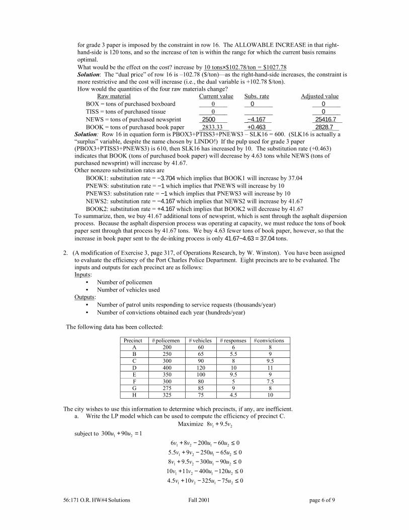
2. (A modification of Exercise 3, page 317, of Operations Research, by W. Winston). You have been assignedto evaluate the efficiency of the Port Charles Police Department. Eight precincts are to be evaluated. Theinputs and outputs for each precinct are as follows:Inputs:
• Number of policemen• Number of vehicles used
Outputs:• Number of patrol units responding to service requests (thousands/year)• Number of convictions obtained each year (hundreds/year)
The following data has been collected:
Precinct # policemen # vehicles # responses # convictionsA 200 60 6 8B 250 65 5.5 9C 300 90 8 9.5D 400 120 10 11E 350 100 9.5 9F 300 80 5 7.5G 275 85 9 8H 325 75 4.5 10
The city wishes to use this information to determine which precincts, if any, are inefficient.a. Write the LP model which can be used to compute the efficiency of precinct C.
1 2Maximize 8 9.5v v+subject to 1 2300 90 1u u+ =
1 2 1 26 8 200 60 0v v u u+ − − ≤
1 2 1 25.5 9 250 65 0v v u u+ − − ≤
1 2 1 28 9.5 300 90 0v v u u+ − − ≤
1 2 1 210 11 400 120 0v v u u+ − − ≤
1 2 1 24.5 10 325 75 0v v u u+ − − ≤

56:171 O.R. HW#4 Solutions Fall 2001 page 7 of 9
1 2 1 29.5 9 350 100 0v v u u+ − − ≤
1 2 1 25 7.5 300 80 0v v u u+ − − ≤
1 2 1 29 8 275 85 0v v u u+ − − ≤
1 2 1 20, 0, 0, 0,u u v v≥ ≥ ≥ ≥
b. What is the total number of LP problems which need to be solved in order to compute the efficienciesof the eight precincts? _8 (one LP per precinct)__
One might use LINDO to do the computation, or any of several other software packages for data envelopmentanalysis—see, for example, the website
http://www.wiso.uni-dortmund.de/lsfg/or/scheel/doordea.htm )The output below was computed by the APL workspace “DEA” which can be downloaded from the website at URL:
http://asrl.ecn.uiowa.edu/dbricker/APL_software.html
i ID Efficiency Freq R1 A 1 4 12 B 1 2 33 C 0.8727 0 64 D 0.809 0 75 E 0.9042 0 56 F 0.6875 0 87 G 1 3 28 H 0.963 0 4
Freq = frequency of appearance in reference sets of inefficient DMUsR = rank based upon (Efficiency + Freq)
Slack inputs/outputs¯¯¯¯¯¯¯¯¯¯¯¯¯¯¯¯¯¯¯¯
i/o C D E F H responses 0 0 0 0 1.61111convictions 0 0 0 0 0 policemen 2.43056 4.86111 22.7083 6.25 35.1852 vehicles 0 0 0 0 0
Prices
i ID responses convictions policemen vehicles 1 A 0.125 0.03125 0.005 0 2 B 0 0.111111 0.00111111 0.0111111 3 C 0.0925926 0.0138889 0 0.0111111 4 D 0.0694444 0.0104167 0 0.008333335 E 0.0833333 0.0125 0 0.01 6 F 0.025 0.075 0 0.0125 7 G 0.0909091 0.0227273 0.00363636 0 8 H 0 0.0962963 0 0.0133333
Reference Sets
For each DMU, the DMUs in its reference set are listed:
3 C 4 D 5 E 6 F 8 H 1 A 1 A 7 G 2 B 2 B 7 G 7 G 1 A 1 A
c. In order to make itself look as “efficient” as possible, what “prices” would be assigned by precinct C tothe outputs (# responses & # convictions) and to the inputs (# policemen & # vehicles)?
Variable Price# responses __0.0925926/thousand responses = 92.5926/response___# convictions __0.0138889/hundred convictions = 13.8889/conviction__# policemen __0/policeman_____# vehicles __0.0111111/vehicle_________
d. Using these prices for precinct C, compute the ratio of the total value of the output variables responsesand convictions to the total value of input variables policemen and vehicles.

56:171 O.R. HW#4 Solutions Fall 2001 page 8 of 9
Solution: 0.092596 8 0.0138889 9.5 0.87271255 87.3%0 300 0.011111 90 1
× + × = ≈× + ×
which is in agreement with the efficiency computed for precinct C.e. Using these same prices which would be assigned by precinct C, which precincts would be judged to
be 100% efficient? Solution: Precincts _A__ and __G__.
f. By how much should precinct C cut its number of policemen in order to become “efficient” (assumingthat they could maintain their current output levels)? Solution: _2.43056__
3. The ZapCon Company is considering investing in three projects. If it fully invests in a project, the realizedcash flows (in millions of dollars) will be as listed in the table below.
Time (years) Cash flow project 1 Cash flow project 2 Cash flow project 30 −3 −2 −2.0
0.5 −1 −0.5 −2.0 1 −1.8 1.5 −1.8
1.5 0.4 1.5 1 2 1.8 1.5 1
2.5 1.8 0.2 1 3 5.5 −1.0 6
For example, project 1 requires an initial cash outflow of $3 million, smaller outlays six months and one yearfrom now, begins paying a small return 1.5 years from now, and a final payback of $5.5 million 3 years fromnow. Today ZapCon has $2 million in cash. At each time point (0, 0.5, 1, 1.5 2, and 2.5 years from today) thecom[any can, if desired, borrow up to $2 million at 3.5% (per 6 months) interest. Leftover cash earns 3% (persix months) interest. For example, if after borrowing and investing at time 0, ZapCon has $1 million, it wouldreceive $30,000 in interest at time 0.5 year. the company’s goal is to maximize cash on hand after cash flows 3years from now are accounted for. What investment and borrowing strategy should it use? Assume that thecompany can invest in a fraction of a project. For example, if it invests in 0.5 of project 3, it has, for example,cash outflows of -$1 million at times 0 and 0.5. No more than 100% investment in a project is possible,however.a. Formulate a linear programming model to optimize the investment plan.Solution: Define variables
F30 = incoming cash flow at time 3.0 yearsPj = investment level in project j, j=1,2,3Bt = amount borrowed ($millions) at time t=00, 05, 10, 15, 20, 25, 30Lt = amount loanded ($millions) at time t=00, 05, 10, 15, 20, 25, 30
For each of the 7 time periods, there is a cash flow balance equation: flow out = flow in. In addition, there areupper bounds of 1 on the variables P1, P2, and P3. (These are best handled as “simple upper bound” (SUB)constraints:
MAX F30SUBJECT TO
2) B00 - 3 P1 - 2 P2 - 2 P3 - L00 = - 23) - 1.035 B00 - P1 - 0.5 P2 - 2 P3 + 1.03 L00 + B05 - L05 = 04) - 1.8 P1 - 0.5 P2 - 2 P3 - 1.035 B05 + 1.03 L05 + B10 - L10 = 05) 0.4 P1 + 1.5 P2 + P3 - 1.035 B10 + 1.03 L10 + B15 - L15 = 06) 1.8 P1 + 1.5 P2 + P3 - 1.035 B15 + 1.03 L15 + B20 - L20 = 07) 1.8 P1 + 0.2 P2 + P3 - 1.035 B20 + 1.03 L20 + B25 - L25 = 08) - F30 + 5.5 P1 - P2 + 6 P3 - 1.035 B25 + 1.03 L25 = 0
ENDSUB P1 1.00000SUB P2 1.00000SUB P3 1.00000
PICTURE command output:
F B L B L B L B L B L B L3 0 P P P 0 0 0 1 1 1 1 2 2 2 20 0 1 2 3 0 5 5 0 0 5 5 0 0 5 5

56:171 O.R. HW#4 Solutions Fall 2001 page 9 of 9
1: 1 ' ' ' ' ' MAX2: 1-3-2-2-1 ' ' ' ' =-23: '-A-1-T-2'A 1-1' ' ' ' ' ' =4: -A-T-2 -A A 1-1 ' ' =5: T A 1 ' -A A 1-1 ' ' =6: ' 'A A 1' ' ' '-A'A 1-1' ' =7: A T 1 ' ' -A A 1-1 =8:-1 A-1 6 ' ' ' -A A =
b. Use LINDO ( or other LP solver) to find the optimal solution.Solution:
OBJECTIVE FUNCTION VALUE1) 7.338224
VARIABLE VALUE REDUCED COSTF30 7.338224 0.000000B00 3.000000 0.000000P1 1.000000 -2.793699P3 1.000000 -2.086015B05 6.105000 0.000000B10 10.118674 0.000000B15 9.072828 0.000000B20 6.590377 0.000000B25 4.021039 0.000000
ROW SLACK OR SURPLUS DUAL PRICES2) 0.000000 -1.2292553) 0.000000 -1.1876864) 0.000000 -1.1475235) 0.000000 -1.1087186) 0.000000 -1.0712257) 0.000000 -1.0350008) 0.000000 -1.000000
The optimal solution is to invest in projects 1 and 3 at their full level. This requires borrowing 3 million dollarsinitially. Additional amounts are borrowed at later points in time, e.g., 10.118 million $ at t = 1 year. The netcash on hand after 3 years is $7,338,224.

56:171 O.R. HW#5 Solutions Fall 2001 page 1 of 5
56:171 Operations ResearchHomework #5 Solutions -- Fall 2001
1. Transportation Problem Consider the following “balanced” transportation problem with three sourcesand four destinations, where the transportation cost/unit shipped, supplies available, and amounts requiredare shown in the table:
Plant \ Warehouse 1 2 3 4 SupplyA 1 4 8 6 7B 1 10 1 7 10C 8 5 6 9 3
Demand 6 6 3 5a. A linear programming model of this problem will have _7_ equality constraints (not counting the
objective) and _6_ basic variables.
b. Find an initial feasible basic solution, using the “Northwest Corner Rule”:Solution
c. The shipping cost of this solution is _____Solution : 6×1+1×4+5×10+3×1+2×7+3×9= 104 .
d. Compute the reduced cost of the variable XA4 by identifying the “cycle” of adjustments that would berequired in the NW-corner solution if XA4 were to be increased by one unit.
Solution: Reduced cost the is +6 −7 +10 −4 = +5.e. Entering XA4 into basis will increase the objective function by _5__ per unit shipped from A to 4.
f. Compute a set of “dual variables” corresponding to the initial NW-corner solution, and use them tocompute the reduced cost of XA4 :
Solution: There are infinitely-many correct answers possible, depending upon the choice of the dualvariable to be given an initial assignment, and the value of that assignment. Here, I have chosen toinitially assign UA=0:XA1>0⇒UA+V1=1⇒V1=1XA2>0⇒UA+V2=4⇒V2=4XB2>0⇒UB+V2=10⇒UB=6XB3>0⇒UB+V3=1⇒V3=−5Etc.Corresponding to supply constraints: UA=__0__, UB=__6_, UC=___8___Corresponding to demand constraints: V1=__1___, V2=__4___, V3=__−5___, V4=__1__
Reduced cost of XA4 is CA4−(UA+V4) = __6__ − _(0+1)__ = _+5__

56:171 O.R. HW#5 Solutions Fall 2001 page 2 of 5
g. The reduced cost of XB1 is is CB1−(UB+V1) = __−6__. Entering XB1 into the basis would cause thevariable _ XB2_ to leave the basis, resulting in the basic solution:
The increase in XA4 (__5_ units) times the reduced cost ( _-6_ ) is _−30__, so that the cost of the newsolution is 104−30= 74.
h. Continue changing the basis until you have found the optimal solution:Solution: Recomputing the dual variables:
Corresponding to supply constraints: UA=__0__, UB=__0_, UC=___2___Corresponding to demand constraints: V1=__1___, V2=__4___, V3=__1___, V4=__7__Using these dual variables, we find that the reduced cost of XC2 is 5−(2+4)=−1<0, and so we enter XC2into the solution: The cycle is more complex than the previous iteration, and three basic variablesdecrease as XC2 increases. The first to reach zero is XC4, when XC2 = 3.
⇒ ⇒Recomputing the dual variables:
Corresponding to supply constraints: UA=__0__, UB=__0_, UC=___1___Corresponding to demand constraints: V1=__1___, V2=__4___, V3=__1___, V4=__7__Reduced cost of XA4 is now –1<0, so we enter this variable into the basis:
⇒Recomputing the dual variables:
Corresponding to supply constraints: UA=__0__, UB=__1_, UC=___1___Corresponding to demand constraints: V1=__0___, V2=__4___, V3=__0___, V4=__6__
The reduced costs are now all nonnegative!i. The optimal cost is _69_ .
2. Powerhouse produces capacitors at three locations: Los Angeles, Chicago, and New York. Capacitors areshipped from these locations to public utilities in five regions of the country: northeast (NE), northwest (NW),midwest (MW), southeast (SE), and southwest (SW). The cost of producing and shipping a capacitor from eachplant to each region of the country is given in the table below.
From \ to NE NW MW SE SWLA $27.86 $4.00 $20.54 $21.52 $13.87Chicago $8.02 $20.54 $2.00 $6.74 $10.67NY $2.00 $27.86 $8.02 $8.41 $15.20
Each plant has an annual production capacity of 100,000 capacitors. Each year, each region of the country mustreceive the following number of capacitors: NE: 55,000; NW: 50,000; MW: 60,000; SE: 60,000; SW: 45,000.

56:171 O.R. HW#5 Solutions Fall 2001 page 3 of 5
Powerhouse feels shipping costs are too high, and the company is therefore considering building one or twomore production plants. Possible sites are Atlanta and Houston. The costs of producing a capacitor andshipping it to each region of the country are:
From \ to NE NW MW SE SWAtlanta $8.41 $21.52 $6.74 $3.00 $7.89Houston $15.20 $13.87 $10.67 $7.89 $3.00
It costs $3 million (in current dollars) to build a new plant, and operating each plant incurs a fixed cost (inaddition to variable shipping and production costs) of $50,000 per year. A plant at Atlanta or Houston will havethe capacity to produce 100,000 capacitors per year.
Assume that future demand patterns and production costs will remain unchanged. If costs are discounted at arate of 11 1/9 % per year, how can Powerhouse minimize the present value of all costs associated with meetingcurrent and future demands?Solution: We may either convert the construction costs of the proposed plants into equivalent annual costs, orconvert the annual costs over an infinite time period into present values. I have arbitrarily selected the latter.With the given discount rate 0.1111111, an infinite sequence of annual costs of $1/year is equivalent to apresent value of ($1/0.111111) = $9.There are four options to consider. For each option, we solve a transportation problem to compute the annualproduction & shipping cost (exclusive of the fixed operating cost and construction costs).
I. No added plants:Shipments
f| to r| ¯¯ o| NE NW MW SE SW dummy m|¯¯¯¯¯ ¯¯¯¯¯ ¯¯¯¯¯ ¯¯¯¯¯ ¯¯¯¯¯ ¯¯¯¯¯1| 0 50000 0 0 20000 300002| 0 0 60000 15000 25000 03|55000 0 0 45000 0 0
Cost = 1453700 ($ per year)Present valueproduction & shipping costs : 9×1453700 = $13,083,300operating costs of plants: 9×3×$50,000 = $1,350,000construction costs: 0Total present value: $14,433,300
II. Add plant at Atlanta onlyShipments
f| to r| ¯¯ o| NE NW MW SE SW dummy m|¯¯¯¯¯ ¯¯¯¯¯ ¯¯¯¯¯ ¯¯¯¯¯ ¯¯¯¯¯ ¯¯¯¯¯1| 0 50000 0 0 0 500002| 0 0 60000 0 5000 350003|55000 0 0 0 0 450004| 0 0 0 60000 40000 0
Cost = 978950 ($ per year)Present valueproduction & shipping costs : 9×978950= $8,810,550operating costs of plants: 9×4×$50,000 = $1,800,000construction cost of Atlanta plant: $3,000,000Total present value: $13,610,550
III. Add plant at Houston onlyShipments

56:171 O.R. HW#5 Solutions Fall 2001 page 4 of 5
f| to r| ¯¯ o| NE NW MW SE SW dummy m|¯¯¯¯¯ ¯¯¯¯¯ ¯¯¯¯¯ ¯¯¯¯¯ ¯¯¯¯¯ ¯¯¯¯¯1| 0 50000 0 0 0 500002| 0 0 60000 40000 0 03|55000 0 0 0 0 450004| 0 0 0 20000 45000 35000
Cost = 992400
Present valueproduction & shipping costs : 9×992400= $8,931,600operating costs of plants: 9×4×$50,000 = $1,800,000construction cost of Houston plant: $3,000,000Total present value: $13,731,600
IV. Add plants at both Atlanta & HoustonShipments
f| to r| ¯¯ o| NE NW MW SE SW dummy m|¯¯¯¯¯ ¯¯¯¯¯ ¯¯¯¯¯ ¯¯¯¯¯ ¯¯¯¯¯ ¯¯¯¯¯1| 0 50000 0 0 0 500002| 0 0 60000 0 0 400003|55000 0 0 0 0 450004| 0 0 0 60000 0 400005| 0 0 0 0 45000 55000
Cost = 745000
Present valueproduction & shipping costs : 9×745,000= $6,705,000operating costs of plants: 9×5×$50,000 = $2,250,000construction cost of Atlanta & Houston plants: $6,000,000Total present value: $14,955,000
The minimum-cost decision is to build the plant at Atlanta. The L.A. plant will then ship 50,000 annually tothe NW region. The Chicago plant will ship 60,000 annually the the MW region and 5000 to the SW region. The NY plant will ship 55,000 to the NE region. The Atlanta plant will ship 60,000 to the SE region and 40,000to the SW region.
3. The coach of a swim team needs to assign four swimmers to a 400-meter medley relay team. The “best times”(in seconds for 100 meters) achieved by his seven swimmers in each of the strokes are given below. Whichswimmer should the coach assign to each of the four strokes? Which swimmers will not be assigned to the relayteam? Are there more than one optimal solution?
Stroke Alan Ben Carl Don Ed Fred GeorgeBackstroke 66 67 66 64 70 68 64Breaststroke 71 72 70 69 72 72 73Butterfly 65 67 71 74 65 64 64Freestyle 59 59 55 59 54 54 56
Solution: This is an assignment problem. Although it isn’t necessary, the matrix has been transposed below, sothat the “agents” correspond to the 7 swimmers and the “tasks” to the four strokes:
Cost matrix:f| to r| ¯¯ o| 1 2 3 4m|¯¯ ¯¯ ¯¯ ¯¯1|66 71 65 592|67 72 67 593|66 70 71 554|64 69 74 595|70 72 65 54

56:171 O.R. HW#5 Solutions Fall 2001 page 5 of 5
6|68 72 64 547|64 73 64 56
m = #agents = 7n = #jobs = 4 3 "Dummy" jobs were definedSince each row already contains a zero, no row reduction is possible/necessary.After column reduction (subtracting 64 from column #1, 69 from column 2, etc.):
2 2 1 5 0 0 03 3 3 5 0 0 02 1 7 1 0 0 00 0 10 5 0 0 06 3 1 0 0 0 04 3 0 0 0 0 00 4 0 2 0 0 0
Seven lines are required to cover all of the zeroes, and so a zero-cost assignment (shown by boxedelements) is possible and therefore optimal.
i -> jGEORGE -> BACKSTROKE DON -> BREASTSTROKE FRED -> BUTTERFLY ED -> FREESTYLE ALAN -> dummy 5 BEN -> dummy 6 CARL -> dummy 7
Minimum Cost = 251Alan, Ben, and Carl are not given positions on the relay team. If all swimmers were to perform at theirbest level, the total time would be 251 seconds. There are no meaningful alternate optimal solutions(except that idle swimmers could be assigned other “dummy” tasks, e.g., ALAN -> dummy 6, etc.)

56:171 O.R. HW#6 Solutions Fall 2001 page 1 of 7
56:171 Operations ResearchHomework #6 Solutions -- Fall 2001
1. Integer LP Model A court decision has stated that the enrollment of each high school in Metropolis be at least20% black. The numbers of black and white high school students in each of the city’s five school districts are:
District Whites Blacks1 80 302 70 53 90 104 50 405 60 30
The distance (in miles) that a student in each district must travel to each high school is:
District HS#1 HS#21 1.0 2.02 0.5 1.73 0.8 0.84 1.3 0.45 1.5 0.6
School board policy requires that all students in a given district must attend the same school, and that each schoolmust have an enrollment of at least 150 students. Formulate an integer LP to determine how to minimize the totaldistance that Metropolis students must travel to high school, and use LINDO (or other ILP solver) to compute theoptimal solution.Decision Variables :
Xij =1 , if students from district i are sent to school j0 , otherwise
Integer Programming Formulation :The objective is to minimize the total distance students travel (which would be equivalent to minimizing the averagedistance traveled), so the coefficient of Xij is the population of district i times the distance from district i to school j.
Min {(80+30)*1.0} X11 + {(70+ 5)*0.5} X21 + {(90+10)*0.8} X31+ {(50+40)*1.3} X41 + {(60+30)*1.5} X51 + {(80+30)*2.0} X12 + {(70+ 5)*1.7} X22 + {(90+10)*0.8} X32+ {(50+40)*0.4} X42 + {(60+30)*0.6} X52
s.t.Minimum enrollment at schools:
(80+30) X11 + (70+5) X21 + (90+10) X31 + (50+40) X41 + (60+30) X51 ≥ 150(80+30) X12 + (70+5) X22 + (90+10) X32 + (50+40) X42 + (60+30) X52 ≥ 150
Minimum proportion of black students in each school:30 X11 + 5 X21 + 10 X31 + 40 X41 + 30 X51
(80+30) X11 + (70+5) X21 + (90+10) X31 + (50+40) X41 + (60+30) X51≥ 0.2
30 X12 + 5 X22 + 10 X32 + 40 X42 + 30 X52(80+30) X12 + (70+5) X22 + (90+10) X32 + (50+40) X42 + (60+30) X52
≥ 0.2
"Multiple choice" constraints: Each district is to be assigned to one of the two schools:X11 + X12 = 1 , X21 + X22 = 1 , X31 + X32 = 1 , X41 + X42 = 1 , X51 + X52 = 1

56:171 O.R. HW#6 Solutions Fall 2001 page 2 of 7
LINDO inputMin 110 X11 + 37.5 X21 + 80 X31 + 117 X41 + 135 X51
+ 220 X12 + 127.5 X22 + 80 X32 + 36 X42 + 54 X52 s.t.110 X11 + 75 X21 + 100 X31 + 90 X41 + 90 X51 >= 150110 X12 + 75 X22 + 100 X32 + 90 X42 + 90 X52 >= 1508X11 - 10X21 - 10X31 + 22X41 + 12X51 >= 08X12 - 10X22 - 10X32 + 22X42 + 12X52 >= 0X11 + X12 = 1X21 + X22 = 1X31 + X32 = 1X41 + X42 = 1X51 + X52 = 1ENDINTE 10
(Here, zero/one variable (binary) restrictions are imposed by the command INTE)
LINDO outputLP OPTIMUM FOUND AT STEP 6OBJECTIVE VALUE = 324.863647
NEW INTEGER SOLUTION OF 398.500000 AT BRANCH 0 PIVOT 6RE-INSTALLING BEST SOLUTION...
OBJECTIVE FUNCTION VALUE
1) 398.5000
VARIABLE VALUE REDUCED COSTX11 1.000000 110.000000X21 1.000000 37.500000X31 0.000000 80.000000X41 1.000000 117.000000X51 0.000000 135.000000X12 0.000000 220.000000X22 0.000000 127.500000X32 1.000000 80.000000X42 0.000000 36.000000X52 1.000000 54.000000
ROW SLACK OR SURPLUS DUAL PRICES2) 125.000000 0.0000003) 40.000000 0.0000004) 20.000000 0.0000005) 2.000000 0.0000006) 0.000000 0.0000007) 0.000000 0.0000008) 0.000000 0.0000009) 0.000000 0.000000
10) 0.000000 0.000000
NO. ITERATIONS= 7BRANCHES= 0 DETERM.= 1.000E 0
Optimal decision : Students from district 1 are sent to school 1,Students from district 2 are sent to school 1,

56:171 O.R. HW#6 Solutions Fall 2001 page 3 of 7
Students from district 3 are sent to school 2,Students from district 4 are sent to school 1,Students from district 5 are sent to school 2.
Corresponding total distance traveled by students is 398.5 miles(which is an average of 0.857 miles for each of the465 students, ranging from 0.5 mile to 1.3 mile.)
❂ ❂ ❂ ❂ ❂ ❂ ❂ ❂ ❂2. Integer LP Model A company sells seven types of boxes, ranging in volume from 17 to 33 cubic feet. Thedemand and size of each box are given below.
Product#: 1 2 3 4 5 6 7Size 33 30 26 24 19 18 17Demand 400 300 500 700 200 400 200
The variable cost (in dollars) of producing each box is equal to the box’s volume. A fixed cost of $1000 is incurredto produce any of a particular box. If the company desires, demand for a box may be satisfied by a box of largersize. Formulate an integer LP model to minimize the cost of meeting the demand for boxes, and solve, usingLINDO (or another ILP solver).
Decision Variables :Xi = the number of type i boxes produced.
Yi =1 , if company produces type i box0 , otherwise
LINDO input
Min 33 X1 + 30 X2 + 26 X3 + 24 X4 + 19 X5 + 18 X6 + 17 X7+ 1000 Y1 + 1000 Y2 + 1000 Y3 + 1000 Y4 + 1000 Y5 + 1000 Y6 + 1000 Y7
Subject toX1 >= 400X1 + X2 >= 700X1 + X2 + X3 >= 1200X1 + X2 + X3 + X4 >= 1900X1 + X2 + X3 + X4 + X5 >= 2100X1 + X2 + X3 + X4 + X5 + X6 >= 2500X1 + X2 + X3 + X4 + X5 + X6 + X7 >= 2700X1 - 2700 Y1 <= 0X2 - 2300 Y2 <= 0X3 - 2000 Y3 <= 0X4 - 1500 Y4 <= 0X5 - 800 Y5 <= 0X6 - 600 Y6 <= 0X7 - 200 Y7 <= 0endinte Y1inte Y2inte Y3inte Y4inte Y5inte Y6inte Y7
LINDO outputLP OPTIMUM FOUND AT STEP 60OBJECTIVE VALUE = 68845.2500
FIX ALL VARS.( 2) WITH RC > 0.000000E+00SET Y2 TO <= 0 AT 1, BND= -0.7047E+05 TWIN=-0.7057E+05 70SET Y3 TO >= 1 AT 2, BND= -0.7122E+05 TWIN=-0.7372E+05 73

56:171 O.R. HW#6 Solutions Fall 2001 page 4 of 7
SET Y4 TO >= 1 AT 3, BND= -0.7175E+05 TWIN=-0.7215E+05 76SET Y5 TO <= 0 AT 4, BND= -0.7250E+05 TWIN=-0.7250E+05 79DELETE Y5 AT LEVEL 4DELETE Y4 AT LEVEL 3DELETE Y3 AT LEVEL 2FLIP Y2 TO >= 1 AT 1 WITH BND= -70566.664SET Y3 TO >= 1 AT 2, BND= -0.7132E+05 TWIN=-0.7232E+05 82SET Y4 TO >= 1 AT 3, BND= -0.7185E+05 TWIN=-0.7225E+05 85SET Y5 TO <= 0 AT 4, BND= -0.7260E+05 TWIN=-0.7260E+05 88DELETE Y5 AT LEVEL 4DELETE Y4 AT LEVEL 3DELETE Y3 AT LEVEL 2DELETE Y2 AT LEVEL 1RELEASE FIXED VARIABLESSET Y2 TO <= 0 AT 1, BND= -0.7082E+05 TWIN=-0.7092E+05 101SET Y3 TO >= 1 AT 2, BND= -0.7157E+05 TWIN=-0.7407E+05 104SET Y4 TO >= 1 AT 3, BND= -0.7210E+05 TWIN=-0.7250E+05 107SET Y5 TO >= 1 AT 4, BND= -0.7210E+05 TWIN=-0.7285E+05 113
NEW INTEGER SOLUTION OF 72100.0000 AT BRANCH 18 PIVOT 113BOUND ON OPTIMUM: 69697.10DELETE Y5 AT LEVEL 4DELETE Y4 AT LEVEL 3DELETE Y3 AT LEVEL 2FLIP Y2 TO >= 1 AT 1 WITH BND= -70916.664SET Y3 TO >= 1 AT 2, BND= -0.7167E+05 TWIN=-0.7267E+05 116SET Y4 TO <= 0 AT 3, BND= -0.7260E+05 TWIN=-0.7220E+05 119DELETE Y4 AT LEVEL 3DELETE Y3 AT LEVEL 2DELETE Y2 AT LEVEL 1ENUMERATION COMPLETE. BRANCHES= 20 PIVOTS= 119
LAST INTEGER SOLUTION IS THE BEST FOUNDRE-INSTALLING BEST SOLUTION...
OBJECTIVE FUNCTION VALUE1) 72100.00
VARIABLE VALUE REDUCED COSTY1 1.000000 1000.000000Y2 0.000000 -5900.000000Y3 1.000000 1000.000000Y4 1.000000 1000.000000Y5 1.000000 1000.000000Y6 0.000000 400.000000Y7 0.000000 600.000000X1 700.000000 0.000000X2 0.000000 0.000000X3 500.000000 0.000000X4 700.000000 0.000000X5 800.000000 0.000000X6 0.000000 0.000000X7 0.000000 0.000000
ROW SLACK OR SURPLUS DUAL PRICES2) 300.000000 0.0000003) 0.000000 -7.0000004) 0.000000 -2.0000005) 0.000000 -5.0000006) 600.000000 0.0000007) 200.000000 0.0000008) 0.000000 -19.0000009) 2000.000000 0.000000

56:171 O.R. HW#6 Solutions Fall 2001 page 5 of 7
10) 0.000000 3.00000011) 1500.000000 0.00000012) 800.000000 0.00000013) 0.000000 0.00000014) 0.000000 1.00000015) 0.000000 2.000000
Optimal decision :700 type 1, 500 type 3, 700 type 4, and 800 type 5 boxes are required to produce to meet the demand. Thecorresponding total cost is $72,100
Note: another formulation might define Y as before, but Z instead of X:
Zij = fraction of type i boxes used to satisfy need for type j boxes
Ci = cost of box of type i
Dj = demand for box of type j
Fi = setup cost for box type i ($1000 in this instance)7 7 7
1 1i i i j ij
i i j iMinimize F Y C D Z
= = =+∑ ∑ ∑
7
. . 7 , 1,...7 or (better) &ij i ij ij i
s t Z Y i Z Y i j=
≤ = ≤ ∀∑
11, 1, 2,...7
j
iji
Z j=
= =∑
{ }0,1 , 0 i,ji ijY Z∈ ≥ ∀
This model is essentially the same as that of the uncapacitated (or “simple”) plant location problem.
❂ ❂ ❂ ❂ ❂ ❂ ❂ ❂ ❂

56:171 O.R. HW#6 Solutions Fall 2001 page 6 of 7
3. Integer LP Model WSP Publishing sells textbooks to college students. WSP has two sales representativesavailable to assign to the seven-state area (states A through G):
The number of college students (in thousands) in each area is indicated in the figure above. Each salesrepresentative must be assigned to two adjacent states. For example, a sales rep could be assigned to A & B, but notA&D. WSP’s goal is to maximize the number of total students in the states assigned to the sales reps. Formulate aninteger LP whose solution will tell WSP where to assign the sales reps. Use LINDO (or another ILP solver) tocompute the optimal assignment.Decision Variables :
Xi =1 , if state i is served by a sales representative0, otherwise
Yij =1 , if an sales representative is assigned to i & j0 , otherwise
Integer Programming Formulation :The objective is to maximize the number of total students in the states assigned to the sales representatives.
Max 34 Xa + 29 Xb + 42 Xc + 21 Xd + 56 Xe + 18 Xf + 21 Xg
s.t.Xj must be zero unless at least one representative is assigned to state i & j.
Xa <= Yab + Yac Xb <= Yab + Ybc + Ybd + YbeXc <= Yac + Ybc + YcdXd <= Ybd + Ycd + Yde + Ydf + YdgXe <= Ybe + Yde + YefXf <= Ydf + Yef + YfgXg <= Ydg + Yfg
Two sales representatives are to be assigned:Yab + Yac + Ybc + Ybd + Ybe + Ycd + Yde + Ydf + Ydg + Yef + Yfg = 2
LINDO inputMax 34 Xa + 29 Xb + 42 Xc + 21 Xd + 56 Xe + 18 Xf + 21 XgSubject toXa - Yab - Yac <= 0Xb - Yab - Ybc - Ybd - Ybe <= 0Xc - Yac - Ybc - Ycd <= 0Xd - Ybd - Ycd - Yde - Ydf - Ydg <= 0Xe - Ybe - Yde - Yef <= 0Xf - Ydf - Yef - Yfg <= 0Xg - Ydg - Yfg <= 0Yab + Yac + Ybc + Ybd + Ybe + Ycd + Yde + Ydf + Ydg + Yef + Yfg = 2
56:171 O.R. HW#6 Solutions Fall 2001 page 7 of 7
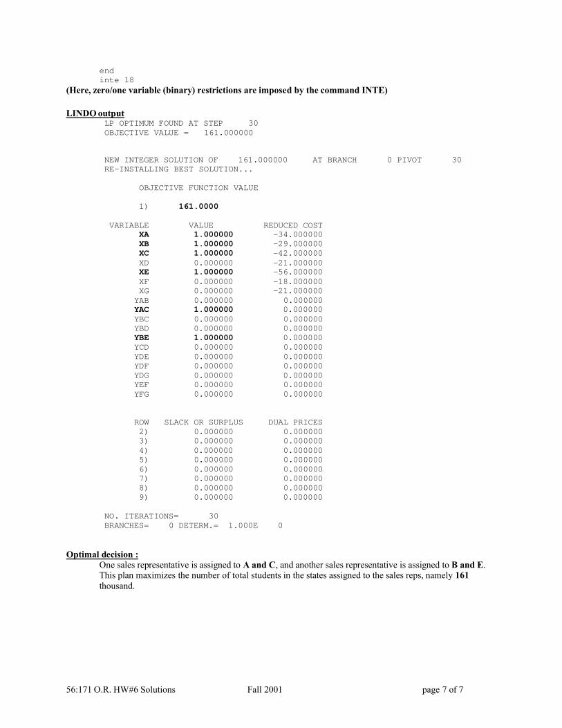
endinte 18
(Here, zero/one variable (binary) restrictions are imposed by the command INTE)
LINDO outputLP OPTIMUM FOUND AT STEP 30OBJECTIVE VALUE = 161.000000
NEW INTEGER SOLUTION OF 161.000000 AT BRANCH 0 PIVOT 30RE-INSTALLING BEST SOLUTION...
OBJECTIVE FUNCTION VALUE
1) 161.0000
VARIABLE VALUE REDUCED COSTXA 1.000000 -34.000000XB 1.000000 -29.000000XC 1.000000 -42.000000XD 0.000000 -21.000000XE 1.000000 -56.000000XF 0.000000 -18.000000XG 0.000000 -21.000000YAB 0.000000 0.000000YAC 1.000000 0.000000YBC 0.000000 0.000000YBD 0.000000 0.000000YBE 1.000000 0.000000YCD 0.000000 0.000000YDE 0.000000 0.000000YDF 0.000000 0.000000YDG 0.000000 0.000000YEF 0.000000 0.000000YFG 0.000000 0.000000
ROW SLACK OR SURPLUS DUAL PRICES2) 0.000000 0.0000003) 0.000000 0.0000004) 0.000000 0.0000005) 0.000000 0.0000006) 0.000000 0.0000007) 0.000000 0.0000008) 0.000000 0.0000009) 0.000000 0.000000
NO. ITERATIONS= 30BRANCHES= 0 DETERM.= 1.000E 0
Optimal decision : One sales representative is assigned to A and C, and another sales representative is assigned to B and E.This plan maximizes the number of total students in the states assigned to the sales reps, namely 161thousand.

56:171 O.R. HW#7 Solutions Fall 2001 page 1 of 5
56:171 Operations ResearchHomework #7 Solutions -- Fall 2001
1. A Markov chain has the transition probability matrix0 0.3 0.7
0.9 0.1 00.2 0 0.8
P =
a. Draw the transition diagram, with probabilities indicated.Solution:
b. Find the probability distributions of the state for the first five steps, given that it begins in state 3.Solution:
2 3 4 5
0.41 0.03 0.56 0.139 0.126 0.735 0.2604 0.0543 0.6853 0.1859 0.08355 0.73050.09 0.28 0.63 , 0.378 0.055 0.567 , 0.1629 0.1189 0.7182 , 0.0.16 0.06 0.78 0.21 0.054 0.736 0.1958 0.0684 0.7858
P P P P = = = =
2507 0.06076 0.68860.2087 0.06558 0.7257
The probability distributions are given by the 3rd row of the matrices P, P2, …P5.c. Find the expected first passage time from state 3 to state 1.
Solution: 4.833 15 1.9051.111 14.5 3.016
5 20 1.381M
=
So the expected number of stages required for the system to reach state 1, given that it begins in state 3, ism31=5.
d. What property does this Markov chain have that guarantees the existence of a steady state probabilitydistribution?Solution: This is a regular Markov chain, indicated by the fact that the elements of P2 are strictly postive.
e. Write the equations which must be solved in order to compute the steady state distribution.Solution:
1 2 2
2 1 2
3 1 3
0.9 0.2, . ., 0.3 0.1
0.7 0.8P i e
π π ππ π π π π
π π π
= += = + = +
(or any two of the preceding equations), and the "normalizing" equation1 2 3 1π π π+ + =
f. What is the steady state probability distribution?Solution: The solution of the system of equations in (e) is

56:171 O.R. HW#7 Solutions Fall 2001 page 2 of 5
1
2
3
0.20690.068970.7241
πππ
= = =
2. An office has two printers, which are very unreliable. It has been observed that when both are working in themorning, there is a 30% chance that one will fail by evening, and a 10% chance that both will fail. If it happensthat only one printer is working in the morning, there is a 20% chance that it will fail by evening. . Any printersthat fail during the day are picked up by a repairman the next morning, and returned the following morning. (Assume that he can work on more than one printer at a time.)
Model this situation as a Markov chain with the state being the number of failed printers observed in the morningafter the repairman has returned any printers but before any failures have occurred. The states then, are 0, 1, & 2.
a. Draw the transition diagram, with probabilities indicated.Solution:
b. Write the transition probability matrix.Solution:
0.6 0.3 0.10.8 0.2 01 0 0
P =
c. What is the probability distribution of the number of failed printers on Wednesday evening if both printersare working on Monday morning?Solution:
3
0.672 0.258 0.070.688 0.248 0.0640.7 0.24 0.06
P =
and so, if both printers are working Monday morning (state 0), there is 67.2% probability that 0 printers arefailed, 25.8% probability that 1 printer is failed, and 7% probability that 2 printers are in the failedcondition on Wednesday evening (after 3 days).
d. What property does this Markov chain have that guarantees the existence of a steady state probabilitydistribution?
Solution: This Markov chain is regular, as evidenced by the fact that P3 has strictly positive elements.e. Write the equations which must be solved in order to compute the steady state distribution.Solution:
1 1 2 3
2 1 2
3 1
0.6 0.80.3 0.20.1
Pπ π π π
π π π π ππ π
= + += ⇒ = + =
and 1 2 3 1π π π+ + =f. What is the steady state probability distribution?Solution:
1
2
3
0.6780.25420.0678
πππ
= = =

56:171 O.R. HW#7 Solutions Fall 2001 page 3 of 5
3. (s,S) Model of Inventory System A periodic inventory replenishment system with reorder point s=2 and order-up to level S=7 is modeled. At the end of each period of demand (day), the inventory is tallied, and if the level isless than or equal to the reorder point (s), enough is ordered (& immediately received) so as to bring the inventorylevel up to S. The probability distribution is discrete and Poisson, with expected demand 2/day.
The state of the system is the inventory position: if no backorders are permitted, as in this case, this is the stock-on-hand. (Otherwise it is the stock-on-hand if nonnegative, and the number of unfilled orders if negative.)
The following output was obtained using the MARKOV workspace (APL code) which is available from the URL:http://asrl.ecn.uiowa.edu/dbricker/APL_software.html
a. Over a long period of time, what is the percent of the days in which you would expect there to be a stockout(zero inventory)? Solution: π0 = 0.09024
b. What will be the average end-of-day inventory level? Solution:7
0
3.443ii
iπ=
=∑c. How often (i.e. once every how many days?) will the inventory be full at the end of the day?
Solution: average interval between visits to state 7 is 777
1 19.17mπ
= = days
d. How often will the inventory be restocked? Solution: The probability that the inventory is re-stocked is2
0
0.09024 +0.09892 +0.1442=0.3333ii
π=
=∑ , which implies that the inventory is restocked, on average, once
every three days.e. If the shelf is full Monday morning, what is the probability that a replenishment occurs Friday evening?Solution: The probability that the system is in states 0, 1, or 2 after 5 stages, given that it begins in state 7, is
7,
2(5)
0
0.08798 +0.09716 +0.1428 = 0.3279j
jp
=
=∑ . Note that this is very nearly the same as the answer to (d)!
f. If the shelf is full Monday morning, what is the probability that the first stockout occurs Friday evening?Solution: The first-passage probability (5)
7,0 0.07153f =
g. What is the expected number of days, starting with a full inventory, until a stockout occurs?Solution: 7,0 11.08m =h. Starting with a full inventory, what is the expected number of stockouts during the first 30 days? What is the
expected number of times that the inventory is restocked? Solution: 30
( )7,0
1
2.619n
np
=
=∑i. What is the average daily cost of this inventory system--including holding cost of $0.50/unit, replenishment
cost of $10 per replenishment, and shortage penalties of $5 per stockout (regardless of the unsatisfieddemand)?
Solution: holding cost7
0
0.50 1.721ii
iπ=
× =∑ $/day
replenishment cost: 2
010 3.3333i
iπ
=
× =∑ $/day
shortage penalties: 05 0.4512π× = $/dayThe sum is 5.505 $/day.If the shortage penalty depended upon the magnitude of the unsatisfied demand, the computation wouldbe somewhat more complicated!

56:171 O.R. HW#7 Solutions Fall 2001 page 4 of 5
Transition Probability Matrix
| 1 2 3 4 5 6 7 8 1 | 0.004534 0.01203 0.03609 0.09022 0.1804 0.2707 0.2707 0.13532 | 0.004534 0.01203 0.03609 0.09022 0.1804 0.2707 0.2707 0.13533 | 0.004534 0.01203 0.03609 0.09022 0.1804 0.2707 0.2707 0.13534 | 0.3233 0.2707 0.2707 0.1353 0 0 0 0 5 | 0.1429 0.1804 0.2707 0.2707 0.1353 0 0 0 6 | 0.05265 0.09022 0.1804 0.2707 0.2707 0.1353 0 0 7 | 0.01656 0.03609 0.09022 0.1804 0.2707 0.2707 0.1353 0 8 | 0.004534 0.01203 0.03609 0.09022 0.1804 0.2707 0.2707 0.1353
Cost Vectori State Cost 1 SOH=zero 10.0 2 SOH=one 10.5 3 SOH=two 11.0 4 SOH=three 1.5 5 SOH=four 2.0 6 SOH=five 2.5 7 SOH=six 3.0 8 SOH=seven 3.5

56:171 O.R. HW#7 Solutions Fall 2001 page 5 of 5
5-th Power| 1 2 3 4 5 6 7 8
1|0.08798 0.09716 0.1428 0.1681 0.1703 0.1606 0.1212 0.051862|0.08798 0.09716 0.1428 0.1681 0.1703 0.1606 0.1212 0.051863|0.08798 0.09716 0.1428 0.1681 0.1703 0.1606 0.1212 0.051864|0.09102 0.09849 0.1418 0.163 0.164 0.1598 0.126 0.055855|0.09283 0.1009 0.1456 0.1667 0.1649 0.156 0.1203 0.0527 6|0.09241 0.1013 0.1473 0.1699 0.1674 0.155 0.1166 0.050167|0.08993 0.09931 0.1457 0.1702 0.1699 0.1575 0.1174 0.049998|0.08798 0.09716 0.1428 0.1681 0.1703 0.1606 0.1212 0.05186
Steady State Distribution| i | state | P{i} | 1 | SOH=zero | 0.09024| 2 | SOH=one | 0.09892| 3 | SOH=two | 0.1442 | 4 | SOH=three | 0.1675 | 5 | SOH=four | 0.1678 | 6 | SOH=five | 0.1585 | 7 | SOH=six | 0.1207 | 8 | SOH=seven | 0.05217
Expected no. of visits during first 30 stages
| 1 2 3 4 5 6 7 8 1|2.619 2.886 4.236 4.982 5.073 4.854 3.73 1.6212|2.619 2.886 4.236 4.982 5.073 4.854 3.73 1.6213|2.619 2.886 4.236 4.982 5.073 4.854 3.73 1.6214|2.888 3.085 4.382 4.945 4.879 4.671 3.59 1.56 5|2.764 3.043 4.428 5.089 4.974 4.613 3.547 1.5426|2.705 2.987 4.384 5.123 5.1 4.695 3.489 1.5177|2.662 2.936 4.31 5.067 5.129 4.82 3.585 1.49 8|2.619 2.886 4.236 4.982 5.073 4.854 3.73 1.621
First Visit Probabilities to State 1 from State 8
n P 1 0.0045342 0.07452 3 0.1048 4 0.08298 5 0.07153 6 0.06623 7 0.05974 8 0.05352 9 0.04818 10 0.0434 11 0.03905 12 0.03514 13 0.03163 14 0.02847 15 0.02562
Mean First Passage Time Matrix| 1 2 3 4 5 6 7 8
1|11.08 10.11 6.936 5.746 5.373 5.305 7.086 19.172|11.08 10.11 6.936 5.746 5.373 5.305 7.086 19.173|11.08 10.11 6.936 5.746 5.373 5.305 7.086 19.174| 8.094 8.101 5.922 5.969 6.529 6.462 8.243 20.325| 9.472 8.527 5.604 5.104 5.959 6.824 8.605 20.696|10.12 9.087 5.911 4.903 5.209 6.311 9.08 21.167|10.6 9.609 6.419 5.239 5.038 5.518 8.287 21.668|11.08 10.11 6.936 5.746 5.373 5.305 7.086 19.17
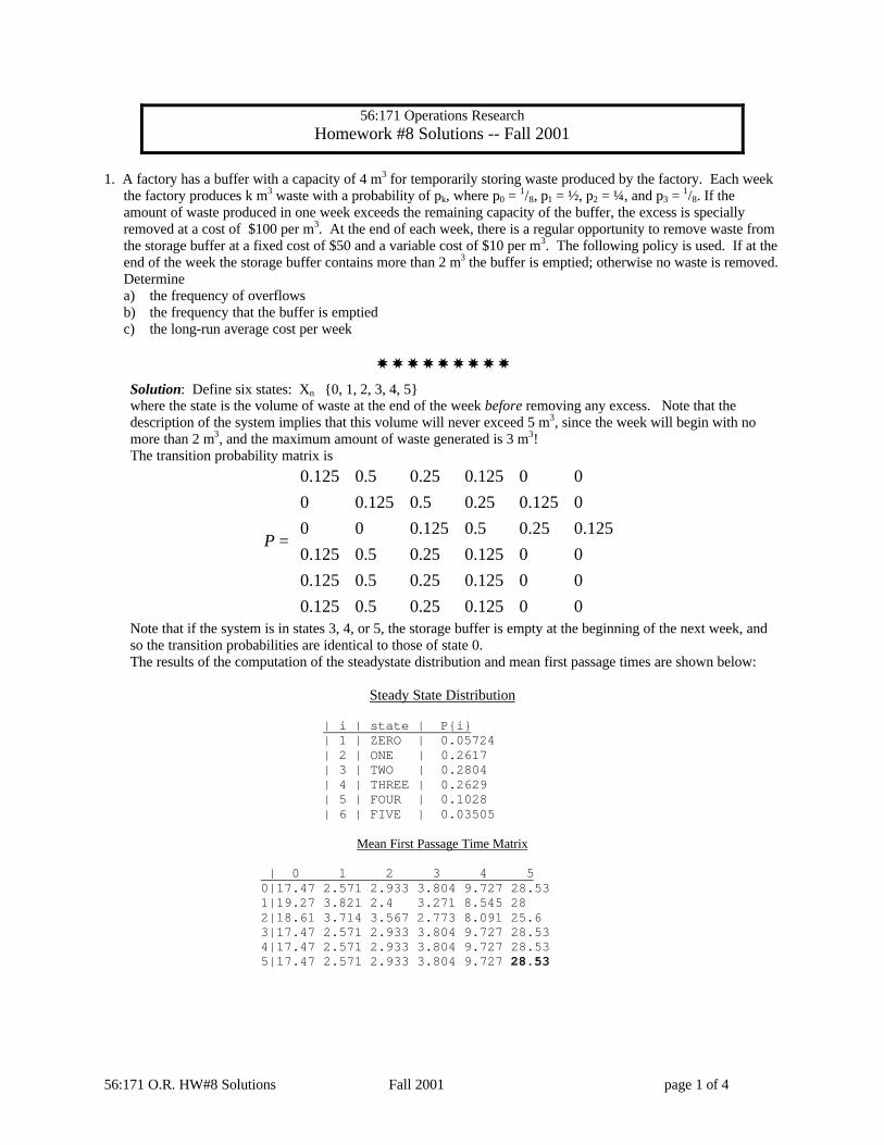
56:171 O.R. HW#8 Solutions Fall 2001 page 1 of 4
56:171 Operations ResearchHomework #8 Solutions -- Fall 2001
1. A factory has a buffer with a capacity of 4 m3 for temporarily storing waste produced by the factory. Each weekthe factory produces k m3 waste with a probability of pk, where p0 = 1/8, p1 = ½, p2 = ¼, and p3 = 1/8. If theamount of waste produced in one week exceeds the remaining capacity of the buffer, the excess is speciallyremoved at a cost of $100 per m3. At the end of each week, there is a regular opportunity to remove waste fromthe storage buffer at a fixed cost of $50 and a variable cost of $10 per m3. The following policy is used. If at theend of the week the storage buffer contains more than 2 m3 the buffer is emptied; otherwise no waste is removed.Determinea) the frequency of overflowsb) the frequency that the buffer is emptiedc) the long-run average cost per week
✸ ✸ ✸ ✸ ✸ ✸ ✸ ✸ ✸
Solution: Define six states: Xn∈{0, 1, 2, 3, 4, 5}where the state is the volume of waste at the end of the week before removing any excess. Note that thedescription of the system implies that this volume will never exceed 5 m3, since the week will begin with nomore than 2 m3, and the maximum amount of waste generated is 3 m3!The transition probability matrix is
0.125 0.5 0.25 0.125 0 0
0 0.125 0.5 0.25 0.125 0
0 0 0.125 0.5 0.25 0.125
0.125 0.5 0.25 0.125 0 0
0.125 0.5 0.25 0.125 0 0
0.125 0.5 0.25 0.125 0 0
P
=
Note that if the system is in states 3, 4, or 5, the storage buffer is empty at the beginning of the next week, andso the transition probabilities are identical to those of state 0.The results of the computation of the steadystate distribution and mean first passage times are shown below:
Steady State Distribution
| i | state | P{i}| 1 | ZERO | 0.05724| 2 | ONE | 0.2617| 3 | TWO | 0.2804| 4 | THREE | 0.2629| 5 | FOUR | 0.1028| 6 | FIVE | 0.03505
Mean First Passage Time Matrix
| 0 1 2 3 4 50|17.47 2.571 2.933 3.804 9.727 28.531|19.27 3.821 2.4 3.271 8.545 282|18.61 3.714 3.567 2.773 8.091 25.63|17.47 2.571 2.933 3.804 9.727 28.534|17.47 2.571 2.933 3.804 9.727 28.535|17.47 2.571 2.933 3.804 9.727 28.53

56:171 O.R. HW#8 Solutions Fall 2001 page 2 of 4
a. The frequency of overflows is the mean recurrence time m55 (= 1/π5 = 28.53) for state 5 (which is the onlystate in which an overflow has occurred.) That is, an overflow occurs, on average, once every 28.53weeks.
b. The frequency with which the buffer is emptied will be the reciprocal of the steadystate probability of statesin which the buffer is emptied, namely states 3, 4, & 5. Thus,
5
3
0.2629 0.1028 0.03505=0.4007ii
π=
= + +∑ ,
so that the buffer is emptied, on average, once every 2.496 weeks.c. The long-run average cost per week is
( ) ( ) ( )3 4 580 90 190 80 0.2629 90 0.1028 190 0.03505
36.94
π π π+ + = × + × + ×
=❋ ❋ ❋ ❋ ❋ ❋ ❋ ❋ ❋ ❋ ❋ ❋ ❋
2. For simplicity, suppose that fresh blood obtained by a hospital will spoil if it is not transfused within five days.The hospital receives 100 pints of fresh blood daily from a local blood bank. Two policies are possible fordetermining the order in which blood is transfused. The following table gives the probabilities of transfusion forblood of various ages under each policy:
0 day old 1 day old 2 days old 3 days old 4 days old
Policy 1 10% 20% 30% 40% 50%
Policy 2 50% 40% 30% 20% 10%
For example, under policy 1, blood has a 10% chance of being transfused during its first day at the hospital.Under policy 2, four-day-old blood has a 10% chance of being transfused.
a. A FIFO (first in, first out) blood-issuing policy issues “old” blood first, whereas a LIFO (last in, first out)policy issues “young” blood first. Which policy above represents a LIFO policy, and which represents aFIFO policy?
Solution: Policy #1 is FIFO and Policy #2 is LIFO.
Define Markov chain models with seven states, where the state is determined when first obtained and every 24hours thereafter.
State Description
1 0 days old
2 1 day old
3 2 days old
4 3 days old
5 4 days old
6 Transfused
7 Spoiled
States 6 & 7 are absorbing states, and states 1 – 5 are transient.
FIFO policy (#1). The transition probability matrix is P=
| 1 2 3 4 5 6 71 | 0 0.9 0 0 0 0.1 02 | 0 0 0.8 0 0 0.2 03 | 0 0 0 0.7 0 0.3 04 | 0 0 0 0 0.6 0.4 05 | 0 0 0 0 0 0.5 0.5

56:171 O.R. HW#8 Solutions Fall 2001 page 3 of 4
6 | 0 0 0 0 0 1 07 | 0 0 0 0 0 0 1
The submatrices Q and R are:
0 0.9 0 0 0 0.1 0
0 0 0.8 0 0 0.2 0
&0 0 0 0.7 0 0.3 0
0 0 0 0 0.6 0.4 0
0 0 0 0 0 0.5 0.5
Q R
= =
Then
( )
1
1
1 0.9 0 0 0 1 0.9 0.72 0.504 0.3024
0 1 0.8 0 0 0 1 0.8 0.56 0.336
0 0 1 0.7 0 0 0 1 0.7 0.42
0 0 0 1 0.6 0 0 0 1 0.6
0 0 0 0 1 0 0 0 0 1
E I Q
−
−
− − = − = =−
−
and
0.8488 0.1512
0.832 0.168
0.79 0.21
0.7 0.3
0.5 0.5
A ER
= =
The first-passage probabilities ( )1,6 , 1,2,3,4,5,6nf n = are
n ( )1,6
nf1 0.12 0.183 0.2164 0.20165 0.15126 0
b. For FIFO policy (#1), the probability that a new pint of blood (state 0) will eventually spoil (reach state 7) isa17=15.12%
c. The average number of pints of blood in inventory may be found from the matrix E: on any typical day, 100% ofthe 100 new pints are in inventory, 90% of the one-day-old pints, 72% of the two-day-old pints, 50.4% of the three-day-old pints, and 30.24% of the four-day-old pints. Thus, the average inventory will be
100+90+72+50.4+30.24=342.6.
d. The average age of transfused blood is the expected first passage time, i.e.,5
( )1,6
1
2.67n
n
n f=
× =∑ days.
✸ ✸ ✸ ✸ ✸ ✸ ✸ ✸ ✸
LIFO policy (#2). The transition probability matrix is P=
| 1 2 3 4 5 6 71 | 0 0.5 0 0 0 0.5 02 | 0 0 0.6 0 0 0.4 03 | 0 0 0 0.7 0 0.3 04 | 0 0 0 0 0.8 0.2 05 | 0 0 0 0 0 0.1 0.96 | 0 0 0 0 0 1 07 | 0 0 0 0 0 0 1
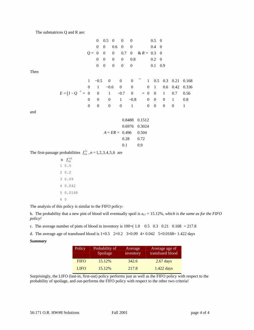
56:171 O.R. HW#8 Solutions Fall 2001 page 4 of 4
The submatrices Q and R are:
0 0.5 0 0 0 0.5 0
0 0 0.6 0 0 0.4 0
&0 0 0 0.7 0 0.3 0
0 0 0 0 0.8 0.2 0
0 0 0 0 0 0.1 0.9
Q R
= =
Then
( )
1
1
1 0.5 0 0 0 1 0.5 0.3 0.21 0.168
0 1 0.6 0 0 0 1 0.6 0.42 0.336
0 0 1 0.7 0 0 0 1 0.7 0.56
0 0 0 1 0.8 0 0 0 1 0.8
0 0 0 0 1 0 0 0 0 1
E I Q
−
−
− − = − = =−
−
and
0.8488 0.1512
0.6976 0.3024
0.496 0.504
0.28 0.72
0.1 0.9
A ER
= =
The first-passage probabilities ( )1,6 , 1,2,3,4,5,6nf n = are
n ( )1,6
nf1 0.5
2 0.2
3 0.09
4 0.042
5 0.0168
6 0
The analysis of this policy is similar to the FIFO policy:
b. The probability that a new pint of blood will eventually spoil is a17 = 15.12%, which is the same as for the FIFOpolicy!
c. The average number of pints of blood in inventory is 100×( 1.0 + 0.5+ 0.3 +0.21+ 0.168) = 217.8
d. The average age of transfused blood is 1×0.5 +2×0.2 +3×0.09+4× 0.042 +5×0.0168= 1.422 days
Summary
Policy Probability ofSpoilage
Averageinventory
Average age oftransfused blood
FIFO 15.12% 342.6 2.67 days
LIFO 15.12% 217.8 1.422 days
Surprisingly, the LIFO (last-in, first-out) policy performs just as well as the FIFO policy with respect to theprobability of spoilage, and out-performs the FIFO policy with respect to the other two criteria!
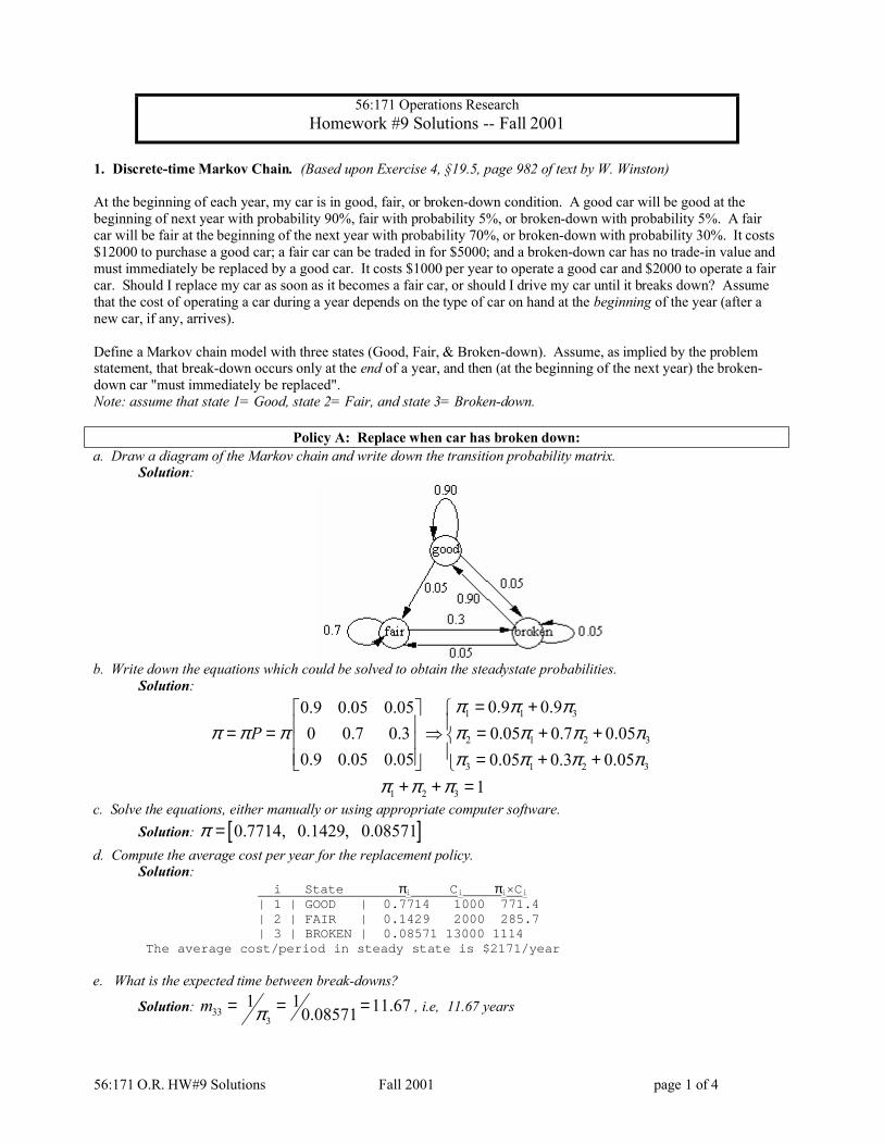
56:171 O.R. HW#9 Solutions Fall 2001 page 1 of 4
56:171 Operations ResearchHomework #9 Solutions -- Fall 2001
1. Discrete-time Markov Chain. (Based upon Exercise 4, §19.5, page 982 of text by W. Winston)
At the beginning of each year, my car is in good, fair, or broken-down condition. A good car will be good at thebeginning of next year with probability 90%, fair with probability 5%, or broken-down with probability 5%. A faircar will be fair at the beginning of the next year with probability 70%, or broken-down with probability 30%. It costs$12000 to purchase a good car; a fair car can be traded in for $5000; and a broken-down car has no trade-in value andmust immediately be replaced by a good car. It costs $1000 per year to operate a good car and $2000 to operate a faircar. Should I replace my car as soon as it becomes a fair car, or should I drive my car until it breaks down? Assumethat the cost of operating a car during a year depends on the type of car on hand at the beginning of the year (after anew car, if any, arrives).
Define a Markov chain model with three states (Good, Fair, & Broken-down). Assume, as implied by the problemstatement, that break-down occurs only at the end of a year, and then (at the beginning of the next year) the broken-down car "must immediately be replaced". Note: assume that state 1= Good, state 2= Fair, and state 3= Broken-down.
Policy A: Replace when car has broken down:a. Draw a diagram of the Markov chain and write down the transition probability matrix.
Solution:
b. Write down the equations which could be solved to obtain the steadystate probabilities.Solution:
1 1 3
2 1 2 3
3 1 2 3
0.9 0.90.9 0.05 0.050 0.7 0.3 0.05 0.7 0.05
0.9 0.05 0.05 0.05 0.3 0.05P
π π ππ π π π π π π
π π π π
= + = = ⇒ = + + = + +
1 2 3 1π π π+ + =c. Solve the equations, either manually or using appropriate computer software.
Solution: [ ]0.7714, 0.1429, 0.08571π =d. Compute the average cost per year for the replacement policy.
Solution:i State πi Ci πi×Ci
| 1 | GOOD | 0.7714 1000 771.4| 2 | FAIR | 0.1429 2000 285.7| 3 | BROKEN | 0.08571 13000 1114
The average cost/period in steady state is $2171/year
e. What is the expected time between break-downs?
Solution: 333
1 1 11.670.08571m π= = = , i.e, 11.67 years

56:171 O.R. HW#9 Solutions Fall 2001 page 2 of 4
Policy B: Replace when car is in FAIR conditiona. Draw a diagram of the Markov chain and write down the transition probability matrix.
Solution:
b. Write down the equations which could be solved to obtain the steadystate probabilities.Solution:
1 1 2 3
2 1 2 3
3 1 2 3
0.9 0.9 0.90.05 0.05 0.050.05 0.05 0.05
Pπ π π π
π π π π π ππ π π π
= + += ⇒ = + + = + +
1 2 3 1π π π+ + =
c. Solve the equations, either manually or using appropriate computer software.Solution: Since each row of P is identical, the solution is obviously [ ]0.9, 0.05, 0.05π =
d. Compute the average cost per year for the replacement policy.Solution:
i State πi Ci πi×Ci| 1 | GOOD | 0.9 1000 900| 2 | FAIR | 0.05 8000 400| 3 | BROKEN | 0.05 13000 650
The average cost/period in steady state is $1950/yearNote that the cost for state 2 FAIR includes the replacement cost (12000) minus trade-in value (5000) plus
the operating cost for the replacement car (1000)!
e. What is the expected time between break-downs?Solution: The probability that the system leaves state 1 is 10%, so it will occur every 10 years
f. What replacement policy do you recommend?Solution:
Policy Average Cost/YearA: Replace when Broken-down $2171B: Replace when in Fair condition $1950
The policy “Replace in FAIR condition” is lower in cost by $221/year.

56:171 O.R. HW#9 Solutions Fall 2001 page 3 of 4
2. Continuous-time Markov Chain. In exercise 1, the Markov chain model assumes that break-down occurs onlyat the end of a year, and then (at the beginning of the next year) the broken-down car "must immediately bereplaced" with a car in good condition. In fact, of course, the change in condition can occur at any time during theyear, and a continuous-time Markov chain model would be a closer representation of reality. Let’s assume thatwhen my car breaks down, it takes me an average of 0.02 years (about 1 week) to find and purchase a replacementcar (and that this delay has exponential distribution.) Again define a Markov chain model with three states (Good,Fair, & Brokendown).
a. What should be the transition rates, so that the probability of a change of condition during a one-year period is inagreement with the probabilities given in exercise 1?
Hint: The cdf of the exponential distribution is
( ) { }time to next event 1 tF t P t e λ−= ≤ = −If in state 1 (good car) there is a 10% probability that the system has changed states during the next year, thetransition rate λ1 should therefore satisfy
( )1 1 0.10F e λ−= − =The value of λ12 should be equal to the value of λ13 (since the transition probabilities p12 and p13 were each5%), and λ1= λ12 + λ13, so λ12= λ13=0.5 λ1. To get the transition rate λ31, observe that the expected value ofthe length of time required to replace my broken-down car is 1/λ31 = 0.02 years.
Solution: Reasoning as above, we obtain:
( ) 1 11 12 13F 1 1 e 0.10 e 0.9 0.1053 0.0526−λ −λ= − = ⇒ = ⇒ λ = ⇒ λ = λ =
( ) 2 22F 1 1 e 0.3 e 0.7 0.3567−λ −λ= − = ⇒ = ⇒ λ =
3131
1 0.02yr 50 / yr= ⇒ λ =λPolicy A: Replace only when broken.
b. Write the matrix of transition rates.Solution: the transition rate matrix is
0.1053 0.0526 0.05260 0.3567 0.3567
50 0 50
− Λ = − −
Note that the diagonal element in each row is chosen to be the negative of the sum of off-diagonal elements.
c. Write the set of equations that must be solved for a steadystate distribution.Solution:
1 3
1 2
1 2 3
0.1053 50 00 0.0526 0.3567 0
0.0526 0.3567 50 0
− π + π =πΛ = ⇒ π − π = π + π − π =
and 1 2 3 1π + π + π =d. Find the steadystate distribution.
Solution: [ ]0.8699, 0.1283, 0.0018π =
e. What does this model predict will be my average operating cost/year (not including replacement costs)?Solution: 1 2($1000 / yr) ($2000 / yr) $1126.45/yrπ + π =
To compute the average replacement costs per year is not quite so simple. (We must multiply the replacement costs bythe expected number of replacements/year, not by π3 (the fraction of the year spent in state 3). Let T = average timebetween replacements. Then

56:171 O.R. HW#9 Solutions Fall 2001 page 4 of 4
3average time from breakdown to replacement 0.02average length of time between replacements
yrT
π = =
What then is T? The number of replacements per year should then be 1/T.
Solution: 3
0.02yr 0.02yr 1T 11.11 yr 0.09 / yr0.0018 T
= = = ⇒ =π
f. What average replacement cost per year is predicted by this model?Solution: $12000×0.09/yr = $1080/yrTotal cost per year with policy A: $1126/yr + $1080/yr = $2206/yr
Policy B: Replace when in FAIR condition.b. The transition rate matrix will be
0.1053 0.0526 0.052650 50 050 0 50
− Λ = − −
c. The equations defining the steadystate distribution will be
1 2 3
1 2
1 3
0.1053 50 50 00.1053 0.0526 0.052650 50 0 0 0.0526 50 050 0 50 0.0526 50 0
− π + π + π =− πΛ = π − = ⇒ π − π = − π − π =
and 1 2 3 1π + π + π =d. Find the steadystate distribution. Solution: [ ]0.9979, 0.00105, 0.00105π =e. What does this model predict will be my average operating cost/year (not including replacement costs)?
Solution: ( $1000/yr)π1 = $997.90/yr
f. What average replacement cost per year is predicted by this model?Solution: As before, the fraction of the time spent replacing the automobile is equal to the ratio 0.02 year to the
cycle length T: 2 32 3
0.02 1 0.1050/yr0.02
yrT T
π ππ π ++ = ⇒ = = ,
i.e., average # replacements/yr is 0.1050The replacement cost when the system reaches state (2) FAIR differs from that in state (3) BROKEN, since atrade-in value is received. Since π2=π3, it appears that half of the replacements result in a trade-in allowance.And so average replacement cost/year will be(0.5× 0.1050/yr × $12000) + (0.5× 0.1050/yr × [12000 - $5000]) = $997.50/yr.
The total expected operating and replacement costs would therefore be $997.90+$997.40 = $1995.40.✸ ✸ ✸ ✸ ✸ ✸ ✸ ✸ ✸
Comparison of Policies:
Policy Average Cost/YearA: Replace when Broken-down $2206B: Replace when in Fair condition $1995
As in exercise 1, Policy B (Replace when in FAIR or BROKEN state) is less costly (by about $211/yr) than Policy A(Replace only when in BROKEN state), and the costs predicted by the continuous-time Markov chain model are onlyslightly higher than those predicted by the discrete-time Markov chain model.

56:171 O.R. HW#10 Solution Fall 2001 page 1 of 5
56:171 Operations ResearchHomework #10 solution-- Fall 2001
1. Birth-death process (exercise 2, section 22.3 of text of Winston. Numerical values modified)My home uses two light bulbs. On average, a light bulb lasts for 30 days (exponentially distributed). When a light
bulb burns out, it takes me an average of 5 days (exponentially distributed) before I replace the bulb (one at atime!)
(rates are in failures/day)
a. Formulate a three-state birth-death model of this situation.Solution: we may define the state of the system to be either the number of bulbs functioning or the numberburned out. (In the diagram above, the state, i.e., “population”, is the number of burned-out bulbs.) Thefailure rate of each bulb is the reciprocal of the average lifetime, i.e., 1/30 per day.
b. Determine the fraction of the time that both light bulbs are working.Solution: To compute the steadystate distribution for this birth-death process, we compute
00
2 2 11 1 1 25 1830 30 301 1 72%1 1 1 3 6 18 255 5 5
ππ
= + + × = + + = ⇒ = =
Then 1 0 2 01 6 1 124% & 4%3 25 6 25
π π π π= = = = = =
c. Determine the fraction of the time that neither light bulb is working.Solution: π2 = 4%d. Suppose that, when both bulbs are burned out and I replace a bulb, I replace both bulbs simultaneously.
Why is this no longer a birth-death process?Solution: The continuous-time Markov chain becomes
which is not a birth-death process, because “deaths” must be one-at-a-time in a birth-death process!

56:171 O.R. HW#10 Solution Fall 2001 page 2 of 5
2. Birth-death process A local takeout Chinese restaurant has space to accommodate at most five customers. During the frigid Iowa winter, it is noticed that when customers arrive and the restaurant is full, virtually no onewaits outside in the subfreezing weather, but instead goes next door to Luigi's Pizza Palace. Customers arrive atthe restaurant at the average rate of 10 per hour, according to a Poisson process. The restaurant servescustomers one at a time, first-come, first-served, in an average of 3 minutes each (the actual time beingexponentially distributed.)
(a.) What is the steady-state distribution of the number of customers in the restaurant?Solution: First compute π0:
( )62 3 4 5
00
111 10 10 10 10 10 21 1.96875 0.5079365 50.8%120 20 20 20 20 1 2
ππ
− = + + + + + = = ⇒ = ≈ −
Population in restaurant Probability0 0.5079371 0.2539682 0.1269843 0.06349214 0.0317465 0.015873
(b.) What is the average number of customers in the Chinese restaurant at any time?
Solution: 5
00.904762i
iL iπ
== =∑
(c.) What is the average arrival rate, considering that when there are 5 customers in the restaurant, the arrivalrate is zero?
Solution: 5
0 1 4 50
10 10 10 0 9.68254i ii
λ λ π π π π π=
= = + + + + =∑ , i.e., 9.68254 customers per hour
(d.) According to Little's Law, what is the expected amount of time that a customer spends in the restaurant?
Solution: 0.904762 0.0934426 hr = 5.60656 min9.68254 /
LL W Whr
λ λ= ⇒ = = =
(e.) What is the fraction of potential customers who are lost to the pizza establishment? Solution: 5 1.6%π ≈What is the number of customers per day lost to the pizza establishment?
Solution: ( ) 510 / 0.16 /hour hourπ× ≈
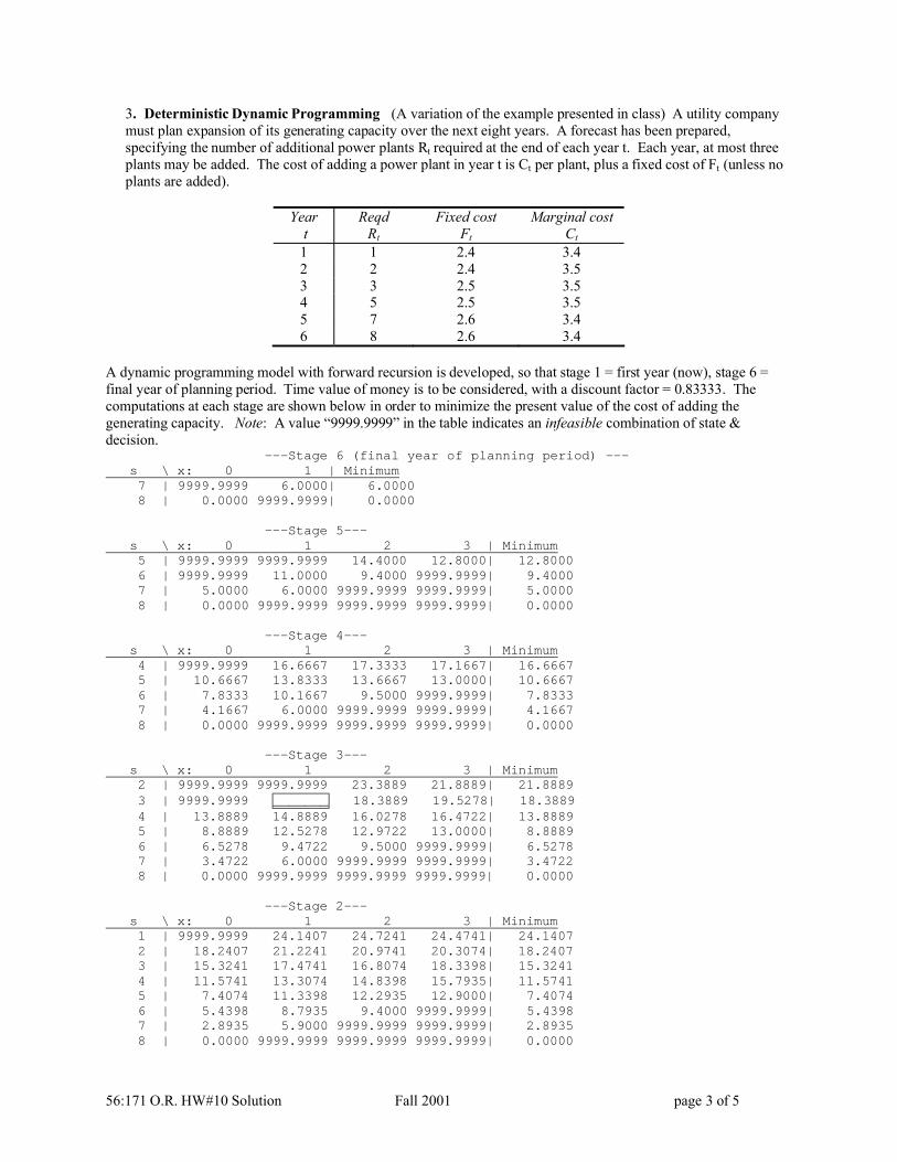
56:171 O.R. HW#10 Solution Fall 2001 page 3 of 5
3. Deterministic Dynamic Programming (A variation of the example presented in class) A utility companymust plan expansion of its generating capacity over the next eight years. A forecast has been prepared,specifying the number of additional power plants Rt required at the end of each year t. Each year, at most threeplants may be added. The cost of adding a power plant in year t is Ct per plant, plus a fixed cost of Ft (unless noplants are added).
Yeart
ReqdRt
Fixed costFt
Marginal costCt
1 1 2.4 3.42 2 2.4 3.53 3 2.5 3.54 5 2.5 3.55 7 2.6 3.46 8 2.6 3.4
A dynamic programming model with forward recursion is developed, so that stage 1 = first year (now), stage 6 =final year of planning period. Time value of money is to be considered, with a discount factor = 0.83333. Thecomputations at each stage are shown below in order to minimize the present value of the cost of adding thegenerating capacity. Note: A value “9999.9999” in the table indicates an infeasible combination of state &decision.
---Stage 6 (final year of planning period) ---s \ x: 0 1 | Minimum7 | 9999.9999 6.0000| 6.0000 8 | 0.0000 9999.9999| 0.0000
---Stage 5---s \ x: 0 1 2 3 | Minimum5 | 9999.9999 9999.9999 14.4000 12.8000| 12.8000 6 | 9999.9999 11.0000 9.4000 9999.9999| 9.4000 7 | 5.0000 6.0000 9999.9999 9999.9999| 5.0000 8 | 0.0000 9999.9999 9999.9999 9999.9999| 0.0000
---Stage 4---s \ x: 0 1 2 3 | Minimum4 | 9999.9999 16.6667 17.3333 17.1667| 16.6667 5 | 10.6667 13.8333 13.6667 13.0000| 10.6667 6 | 7.8333 10.1667 9.5000 9999.9999| 7.8333 7 | 4.1667 6.0000 9999.9999 9999.9999| 4.1667 8 | 0.0000 9999.9999 9999.9999 9999.9999| 0.0000
---Stage 3---s \ x: 0 1 2 3 | Minimum2 | 9999.9999 9999.9999 23.3889 21.8889| 21.8889 3 | 9999.9999 _______ 18.3889 19.5278| 18.3889 4 | 13.8889 14.8889 16.0278 16.4722| 13.8889 5 | 8.8889 12.5278 12.9722 13.0000| 8.8889 6 | 6.5278 9.4722 9.5000 9999.9999| 6.5278 7 | 3.4722 6.0000 9999.9999 9999.9999| 3.4722 8 | 0.0000 9999.9999 9999.9999 9999.9999| 0.0000
---Stage 2---s \ x: 0 1 2 3 | Minimum1 | 9999.9999 24.1407 24.7241 24.4741| 24.1407 2 | 18.2407 21.2241 20.9741 20.3074| 18.2407 3 | 15.3241 17.4741 16.8074 18.3398| 15.3241 4 | 11.5741 13.3074 14.8398 15.7935| 11.5741 5 | 7.4074 11.3398 12.2935 12.9000| 7.4074 6 | 5.4398 8.7935 9.4000 9999.9999| 5.43987 | 2.8935 5.9000 9999.9999 9999.9999| 2.8935 8 | 0.0000 9999.9999 9999.9999 9999.9999| 0.0000

56:171 O.R. HW#10 Solution Fall 2001 page 4 of 5
---Stage 1 (first year of planning period )---s \ x: 0 1 2 3 | Minimum0 | 9999.9999 25.9173 24.4006 25.3701| 24.4006
a. What annual percent return on investment is implied by the discount factor β = 0.833333?
Solution: 1 1 1 20%1
rr
ββ
= ⇒ = − =+
b. One value is missing in the table, i.e., the total cost of years 3, 4, 5, and 6 if, at the beginning of year 3, thecompany has already added 3 plants and decides to add 1 additional plant. What is this value?
Construction cost in year 3 2.5 + 3.5 = 6
Discounted minimum cost of years 4, 5, & 6 β×f4(4) = 0.83333×16.6667 = 13.8889
Total 19.8889
b. What is the minimum present value of the total construction cost to meet the requirements?
Solution: f1(0) = 24.4006
c. What is the optimal schedule for adding plants?
Solution: The “minimum” column in each table above displays the value
Fn(s) = minimum cost of stages n, n+1, …8 if s plants are already built at the beginning of stage n
and the column in which this minimum was found indicates the optimal decision at that stage.
One could, therefore, determine tables for all the optimal values and decisions:
Stage 1Current Optimal Optimal NextState Decision Value State0 added Build 2 24.4006 2 added
Stage 2Current Optimal Optimal Next State Decision Value State 1 added Build 1 24.1407 2 added 2 added Idle 18.2407 2 added 3 added Idle 15.3241 3 added4 added Idle 11.5741 4 added 5 added Idle 7.4074 5 added 6 added Idle 5.4398 6 added 7 added Idle 2.8935 7 added 8 added Idle 0.0000 8 added
Stage 3Current Optimal Optimal Next State Decision Value State 2 added Build 3 21.8889 5 added 3 added Build 2 18.3889 5 added 4 added Idle 13.8889 4 added 5 added Idle 8.8889 5 added 6 added Idle 6.5278 6 added 7 added Idle 3.4722 7 added 8 added Idle 0.0000 8 added

56:171 O.R. HW#10 Solution Fall 2001 page 5 of 5
Stage 4Current Optimal Optimal Next State Decision Value State 4 added Build 1 16.6667 5 added 5 added Idle 10.6667 5 added 6 added Idle 7.8333 6 added 7 added Idle 4.1667 7 added 8 added Idle 0.0000 8 added
Stage 5Current Optimal Optimal Next State Decision Value State 5 added Build 3 12.8000 8 added 6 added Build 2 9.4000 8 added 7 added Idle 5.0000 7 added 8 added Idle 0.0000 8 added
Stage 6Current Optimal Optimal Next State Decision Value State 7 added Build 1 6.0000 8 added 8 added Idle 0.0000 8 added
We can then trace through the table to find the optimal schedule for adding capacity:
Year t # plants toadd
Cumulative #plants added
# plantsrequired
1 2 2 1
2 0 2 2
3 3 5 3
4 0 5 5
5 3 8 7
6 0 8 8
d. Suppose that (for unspecified reasons) the number of plants added during the first year is one (not optimal!). What is the best schedule for adding capacity during the remaining five years?
Solution: If the system begins stage 2 in state 1, we can trace through the tables beginning with stage 2 in order toobtain the following schedule for adding capacity:
Year t # plants toadd
Cumulative #plants added
# plantsrequired
1 1 1 1
2 1 2 2
3 3 5 3
4 0 5 5
5 3 8 7
6 0 8 8

56:171 O.R. HW#11 Fall 2001 page 1 of 6
56:171 Operations ResearchHomework #11 Solution -- Fall 2001
1. Redistricting Problem A state is to be allocated twenty representatives (Reps) to be sent to the nationallegislature. There are nine districts within the state, whose boundaries are fixed. Every district should be assignedat least one representative. The allocation should be done according to the population (Pop) of the districts:
District 1 2 3 4 5 6 7 8 9Population 50 60 70 50 70 100 20 70 40
The "target allocation" of district i is Reps times Pop[i] divided by the population of the state, but this target isgenerally non-integer. The objective is the assign the representatives to the districts in such a way that themaximum absolute deviation from the targets is as small as possible. In the DP model, there is a stage for each district, and the state of the system is the number of representatives not yetassigned when we decide upon the allocation to district i. The optimal value function is defined by a forwardrecursion:
( ){ }
( ){ }( ) ( )
n 1x 1,2,3,4
0 0
minimum max ,
0 0 & for 0
n nf s x f s x
f f s s
+∈ = α − −
= = +∞ >That is, the optimal value function ( )nf s at stage n with state s is the smallest possible value of the maximumabsolute deviations from the targets α of the allocation to districts n, n+1, …. 9 if the total number ofrepresentatives available to those districts is given by the state s.
a. What is the “target” allocation αi of each district?District 1 2 3 4 5 6 7 8 9Population 50 60 70 50 70 100 20 70 40Target 1.88 2.26 2.64 1.88 2.64 3.77 0.75 2.64 1.51Rounded: 2 2 3 2 3 4 1 3 2
Note that by rounding the “target” to the nearest integer, the number of representatives allocated is 22 (>20!)b. Compute the missing values in the table below for stage 3.Solution: The target allocation α3 is 2.64. Therefore:(s=12, x=1): ( ){ } ( ){ } { }n 1 4max , max 2.64 1 , 11 max 1.64,0.77 1.64nx f s x f+α − − = − = =
(s=12, x=2): ( ){ } { }4max 2.64 2 , 10 max 0.64,0.89 0.89f− = =
(s=12, x=3): ( ){ } { }4max 2.64 3 , 9 max 0.36,1.64 1.64f− = =
(s=12, x=1): ( ){ } { }4max 2.64 1 , 11 max 1.64,0.77 1.64f− = =
(s=13, x=1): ( ){ } ( ){ } { }n 1 4max , max 2.64 1 , 12 max 1.64,0.64 1.64nx f s x f+α − − = − = = , etc.c. There are three optimal solutions to this problem. For each solution, what are the optimal allocations ofrepresentatives to districts? (Enter in tables below.)Solution #1:
District 1 2 3 4 5 6 7 8 9Allocation 2 2 2 2 3 4 1 3 1Deviation +0.12 −0.26 −0.64 +0.12 +0.36 +0.23 +0.25 +0.36 −0.51
Solution #2:District 1 2 3 4 5 6 7 8 9Allocation 2 2 3 2 2 4 1 3 1Deviation +0.12 −0.26 +0.36 +0.12 −0.64 +0.23 +0.25 +0.36 −0.51
Solution #3:District 1 2 3 4 5 6 7 8 9Allocation 2 2 3 2 3 4 1 2 1Deviation +0.12 −0.26 +0.36 +0.12 +0.36 +0.23 +0.25 −0.64 −0.51

56:171 O.R. HW#11 Fall 2001 page 2 of 6
d. Does one of the three solutions seem “better” than the others with respect to some other considerations? ???? They seem very comparable to me in every way!
e. Which district has the largest positive deviation from its target allocation?Solution #1: district 3; Solution #2: District 5; Solution #3: District 8
f. Which district has the largest negative deviation from its target allocation? Same as (e)—in every case, thedeviation with the maximumabsolute value is negative, i.e., the district is underrepresented.
---Stage 9---s \ x: 1 2 3 4 | Min1 | 0.51 999.99 999.99 999.99| 0.51 2 | 999.99 0.49 999.99 999.99| 0.49 3 | 999.99 999.99 1.49 999.99| 1.49 4 | 999.99 999.99 999.99 2.49| 2.49
---Stage 8---s \ x: 1 2 3 4 | Min2 | 1.64 999.99 999.99 999.99| 1.64 3 | 1.64 0.64 999.99 999.99| 0.64 4 | 1.64 0.64 0.51 999.99| 0.51 5 | 2.49 1.49 0.49 1.36| 0.49 6 | 999.99 2.49 1.49 1.36| 1.36 7 | 999.99 999.99 2.49 1.49| 1.49 8 | 999.99 999.99 999.99 2.49| 2.49
---Stage 7---s \ x: 1 2 3 4 | Min3 | 1.64 999.99 999.99 999.99| 1.64 4 | 0.64 1.64 999.99 999.99| 0.64 5 | 0.51 1.25 2.25 999.99| 0.51 6 | 0.49 1.25 2.25 3.25| 0.49 7 | 1.36 1.25 2.25 3.25| 1.25 8 | 1.49 1.36 2.25 3.25| 1.36 9 | 2.49 1.49 2.25 3.25| 1.49
10 | 999.99 2.49 2.25 3.25| 2.25 11 | 999.99 999.99 2.49 3.25| 2.49 12 | 999.99 999.99 999.99 3.25| 3.25
---Stage 6---s \ x: 1 2 3 4 | Min4 | 2.77 999.99 999.99 999.99| 2.77 5 | 2.77 1.77 999.99 999.99| 1.77 6 | 2.77 1.77 1.64 999.99| 1.64 7 | 2.77 1.77 0.77 1.64| 0.77 8 | 2.77 1.77 0.77 0.64| 0.64 9 | 2.77 1.77 0.77 0.51| 0.51 10 | 2.77 1.77 1.25 0.49| 0.49 11 | 2.77 1.77 1.36 1.25| 1.25 12 | 2.77 2.25 1.49 1.36| 1.36 13 | 3.25 2.49 2.25 1.49| 1.49 14 | 999.99 3.25 2.49 2.25| 2.25 15 | 999.99 999.99 3.25 2.49| 2.49
---Stage 5---s \ x: 1 2 3 4 | Min5 | 2.77 999.99 999.99 999.99| 2.77 6 | 1.77 2.77 999.99 999.99| 1.77 7 | 1.64 1.77 2.77 999.99| 1.64 8 | 1.64 1.64 1.77 2.77| 1.64 9 | 1.64 0.77 1.64 1.77| 0.77 10 | 1.64 0.64 0.77 1.64| 0.64 11 | 1.64 0.64 0.64 1.36| 0.64 12 | 1.64 0.64 0.51 1.36| 0.51 13 | 1.64 1.25 0.49 1.36| 0.49 14 | 1.64 1.36 1.25 1.36| 1.25 15 | 2.25 1.49 1.36 1.36| 1.36 16 | 2.49 2.25 1.49 1.36| 1.36
---Stage 4---s \ x: 1 2 3 4 | Min8 | 1.64 1.77 2.77 999.99| 1.64 9 | 1.64 1.64 1.77 2.77| 1.64 10 | 0.89 1.64 1.64 2.11| 0.89 11 | 0.89 0.77 1.64 2.11| 0.77 12 | 0.89 0.64 1.11 2.11| 0.64 13 | 0.89 0.64 1.11 2.11| 0.64 14 | 0.89 0.51 1.11 2.11| 0.51 15 | 1.25 0.49 1.11 2.11| 0.49 16 | 1.36 1.25 1.11 2.11| 1.11 17 | 1.36 1.36 1.25 2.11| 1.25 1.64 0.89 1.64 1.64 1.64
---Stage 3---s \ x: 1 2 3 4 | Min12 | 1.64 0.89 1.64 1.64| 0.89 13 | 1.64 0.77 0.89 1.64| 0.77 14 | 1.64 0.64 0.77 1.36| 0.64 15 | 1.64 0.64 0.64 1.36| 0.64 16 | 1.64 0.64 0.64 1.36| 0.64 17 | 1.64 0.64 0.51 1.36| 0.51 18 | 1.64 1.11 0.49 1.36| 0.49
---Stage 2---s \ x: 1 2 3 4 | Min16 | 1.26 0.64 0.77 1.74| 0.64 17 | 1.26 0.64 0.74 1.74| 0.64 18 | 1.26 0.64 0.74 1.74| 0.64 19 | 1.26 0.51 0.74 1.74| 0.51
---Stage 1---s \ x: 1 2 3 4 | Min20 | 0.89 0.64 1.11 2.11| 0.64
✜ ✜ ✜ ✜ ✜ ✜ ✜ ✜ ✜ ✜ ✜ ✜ ✜ ✜ ✜ ✜ ✜ ✜

56:171 O.R. HW#11 Fall 2001 page 3 of 6
2. (Deterministic) Equipment Replacement. The optimal policy for replacement of a machine over the next tenyears is required. The cost of a new machine is $10,000. The table below indicates the annual operating cost ofthe machine, and the trade-in value, according to its age. The policy is to keep a machine for no more than sixyears. A new machine has just been purchased (whose cost should not be considered), and at the end of the ten-year planning period, a new machine is required.
Age of machine (yrs) Operating cost/year ($) Trade-in value ($)0 1400 75001 1800 60002 2400 50003 3000 42004 3500 35005 4000 25006 4500 0
a. What is the total cost of the policy which replaces the machine at the end of year 5 and year 10?
Define the functionsg(n) = minimum total operating & replacement cost (including trade-in value) if, with n years remaining in the
planning period, you have a new machiney(n) = optimal age at which the machine is to be replaced if, with n years remaining in the planning period,
you have a new machine.Yrs to go (n) g(n) y(n)
10 25600 2, 3, or 49 21800 38 18400 2 or 37 15000 2, 3, or 46 11200 35 7800 2 or 34 4400 2 or 43 600 32 −2800 21 −6100 10 0
For example, if n=2 years remain with a new machine, which is replaced at the end of two years, i.e.,y(2)=2, the total cost is: operating cost: 1400+1800 = 3400cost of new machine: 10000trade-in value: −2500
Total: 7200
b. Complete the computations in the table above. Solution: see above.For example, when n=8:
If y= 1 2 3 4 5 6then OC= 1400 3200 5600 8600 12100 16100and RC= 2500 4000 5000 5800 6500 7500and g(8-y) = 15000 11200 7800 4400 600 −2800So total= 18900 18400 18400 18800 19200 20800
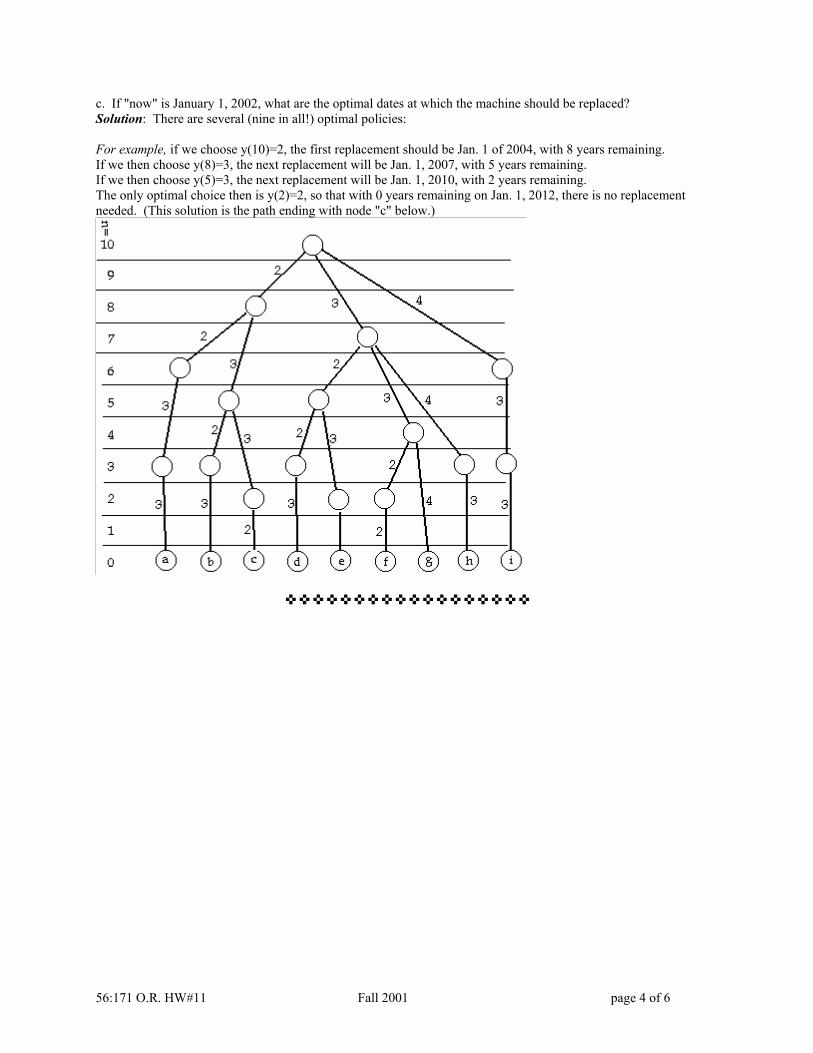
56:171 O.R. HW#11 Fall 2001 page 4 of 6
c. If "now" is January 1, 2002, what are the optimal dates at which the machine should be replaced?Solution: There are several (nine in all!) optimal policies:
For example, if we choose y(10)=2, the first replacement should be Jan. 1 of 2004, with 8 years remaining.If we then choose y(8)=3, the next replacement will be Jan. 1, 2007, with 5 years remaining.If we then choose y(5)=3, the next replacement will be Jan. 1, 2010, with 2 years remaining.The only optimal choice then is y(2)=2, so that with 0 years remaining on Jan. 1, 2012, there is no replacementneeded. (This solution is the path ending with node "c" below.)
✜ ✜ ✜ ✜ ✜ ✜ ✜ ✜ ✜ ✜ ✜ ✜ ✜ ✜ ✜ ✜ ✜ ✜

56:171 O.R. HW#11 Fall 2001 page 5 of 6
3. Stochastic Production Planning. The state of the system is the "inventory position", which if positive is thestock on hand, and if negative is the number of backorders which have accumulated, which is observed at the end ofthe business day. The decision is the number of units to be produced, which is no more than 3. There is a setupcost of $10 if any units are produced, plus $4 per unit. We assume that production is completed in time to meet anydemand that occurs the next day. The demand is a discrete random variable with stationary distribution
D 0 1 2 3 4P{D} 0.1 0.2 0.3 0.2 0.2
In addition, there is a storage cost of $1 per unit, based upon the end-of-day inventory, and a shortage cost of $15per unit, based upon any backorders. Finally, at the end of the planning period (5 days), a salvage value of $2 perunit is received for any remaining inventory. If any shortage exists at the end of the planning period, enough mustbe produced to satisfy that shortage. A backward recursion is used, where F(N) is a vector (one element per state) containing the minimum expected costof the final N days of the planning period if the initial inventory position corresponds to that state. Initially, with 5 days remaining (i.e., stage 5) there are 2 units in inventory.
Below are the tables used to compute the optimal production policy.
a. What is the missing value in the table for stage 1? _22.80_Production cost (x=2): 10+2×4 = 18Storage cost (s=1): 1If demand = 0, final state is 3, so salvage value is -6If demand = 1, final state is 2, so salvage value is -4If demand = 2, final state is 1, so salvage value is -2If demand = 3, final state is 0, so cost = 0If demand = 4, final state is -1, i.e., shortage of 1 unit, so cost is 15 shortage cost + 14 production cost=29Total expected cost: 19 + (0.1×(−6)) + (0.2×(−4)) + (0.3×(−2)) + (0.2×0) + (0.2×29) = 19+3.8 =22.8
b. What is the missing value in the table for stage 5? _93.32_Production cost (x=2): 10+2×4 = 18Storage cost (s=2): 2If demand = 0, final state is 4, and f4(4) = 58.01If demand = 1, final state is 3, and f4(3) = 65.84If demand = 2, final state is 2, and f4(2) = 71.10If demand = 3, final state is 1, and f4(1) = 77.01If demand = 4, final state is 0, and f4(0) = 88.09Total expected cost: 20 + (0.1×58.01) + (0.2×65.84) + (0.3×71.10) + (0.2×77.01) + (0.2×88.09)
= 20 + 73.32 = 93.32
c. What is the optimal production decision at the initial stage (stage 5)? _produce 3_
d. What is the minimum expected cost (total of production, storage, and shortage costs) for the five-day period?__90.18__
e. Suppose that the demand in the first day (i.e., stage 5) is 1. What is the optimal production decision for day 2(i.e., stage 4)? _0_ The quantity available to satisfy the first day's demand is 2+3=5. If the demand is 1, then thesecond day is begun with stock-on-hand = 4, and according to the table for stage 4, the optimal production quantityis 0.

56:171 O.R. HW#11 Fall 2001 page 6 of 6
---Stage 1---s \ x: 0 1 2 3 | Minimum¯3 | 9999.99 9999.99 9999.99 114.00| 114.00 ¯2 | 9999.99 9999.99 95.00 83.50| 83.50 ¯1 | 9999.99 76.00 64.50 51.60| 51.60 0 | 47.00 45.50 32.60 25.80| 25.80 1 | 32.50 29.60 22.80 19.40| 19.40 2 | 16.60 19.80 16.40 18.40| 16.40 3 | 6.80 13.40 15.40 17.40| 6.80 4 | 0.40 12.40 14.40 16.60| 0.40 5 | ¯0.60 11.40 13.60 16.20| ¯0.60 6 | ¯1.60 10.60 13.20 16.40| ¯1.60
---Stage 2---s \ x: 0 1 2 3 | Minimum¯3 | 9999.99 9999.99 9999.99 150.55| 150.55 ¯2 | 9999.99 9999.99 131.55 114.08| 114.08 ¯1 | 9999.99 112.55 95.08 77.28| 77.28 0 | 83.55 76.08 58.28 47.26| 47.26 1 | 63.08 55.28 44.26 38.36| 38.36 2 | 42.28 41.26 35.36 33.22| 33.22 3 | 28.26 32.36 30.22 29.48| 28.26 4 | 19.36 27.22 26.48 26.78| 19.36 5 | 14.22 23.48 23.78 26.00| 14.22 6 | 10.48 20.78 23.00 26.60| 10.48
---Stage 3---s \ x: 0 1 2 3 | Minimum¯3 | 9999.99 9999.99 9999.99 181.63| 181.63 ¯2 | 9999.99 9999.99 162.63 141.40| 141.40 ¯1 | 9999.99 143.63 122.40 100.44| 100.44 0 | 114.63 103.40 81.44 67.89| 67.89 1 | 90.40 78.44 64.89 57.68| 57.68 2 | 65.44 61.89 54.68 52.09| 52.09 3 | 48.89 51.68 49.09 47.00| 47.00 4 | 38.68 46.09 44.00 42.93| 38.68 5 | 33.09 41.00 39.93 40.00| 33.09 6 | 28.00 36.93 37.00 39.23| 28.00
---Stage 4---s \ x: 0 1 2 3 | Minimum¯3 | 9999.99 9999.99 9999.99 208.95| 208.95 ¯2 | 9999.99 9999.99 189.95 166.08| 166.08 ¯1 | 9999.99 170.95 147.08 122.48| 122.48 0 | 141.95 128.08 103.48 88.09| 88.09 1 | 115.08 100.48 85.09 77.01| 77.01 2 | 87.48 82.09 74.01 71.10| 71.10 3 | 69.09 71.01 68.10 65.84| 65.84 4 | 58.01 65.10 62.84 61.46| 58.01 5 | 52.10 59.84 58.46 58.15| 52.10 6 | 46.84 55.46 55.15 57.01| 46.84
---Stage 5---s \ x: 0 1 2 3 | Minimum2 | 108.65 102.02 93.32 90.18| 90.18
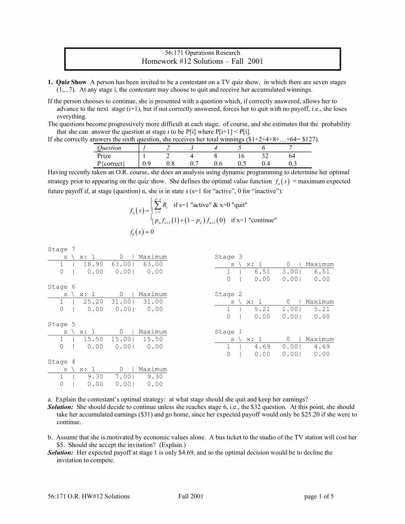
56:171 O.R. HW#12 Solutions Fall 2001 page 1 of 5
56:171 Operations ResearchHomework #12 Solutions – Fall 2001
1. Quiz Show A person has been invited to be a contestant on a TV quiz show, in which there are seven stages(1,...7). At any stage i, the contestant may choose to quit and receive her accumulated winnings.
If the person chooses to continue, she is presented with a question which, if correctly answered, allows her toadvance to the next stage (i+1), but if not correctly answered, forces her to quit with no payoff, i.e., she loseseverything.
The questions become progressively more difficult at each stage, of course, and she estimates that the probabilitythat she can answer the question at stage i to be P[i] where P[i+1] < P[i].
If she correctly answers the sixth question, she receives her total winnings ($1+2+4+8+…+64= $127). Question 1 2 3 4 5 6 7Prize 1 2 4 8 16 32 64P{correct} 0.9 0.8 0.7 0.6 0.5 0.4 0.3
Having recently taken an O.R. course, she does an analysis using dynamic programming to determine her optimalstrategy prior to appearing on the quiz show. She defines the optimal value function ( )nf s = maximum expectedfuture payoff if, at stage (question) n, she is in state s (s=1 for “active”, 0 for “inactive”):
( )( ) ( ) ( )
( )
1
1
1 1
8
if s=1 "active" & x=0 "quit"
1 1 0 if x=1 "continue"
0
n
iin
n n n n
Rf s
p f p f
f s
−
=
+ +
= + −
=
∑
Stage 7s \ x: 1 0 | Maximum1 | 18.90 63.00| 63.00 0 | 0.00 0.00| 0.00
Stage 6s \ x: 1 0 | Maximum1 | 25.20 31.00| 31.00 0 | 0.00 0.00| 0.00
Stage 5s \ x: 1 0 | Maximum1 | 15.50 15.00| 15.50 0 | 0.00 0.00| 0.00
Stage 4s \ x: 1 0 | Maximum1 | 9.30 7.00| 9.30 0 | 0.00 0.00| 0.00
Stage 3s \ x: 1 0 | Maximum1 | 6.51 3.00| 6.51 0 | 0.00 0.00| 0.00
Stage 2s \ x: 1 0 | Maximum1 | 5.21 1.00| 5.21 0 | 0.00 0.00| 0.00
Stage 1s \ x: 1 0 | Maximum1 | 4.69 0.00| 4.69 0 | 0.00 0.00| 0.00
a. Explain the contestant’s optimal strategy: at what stage should she quit and keep her earnings?Solution: She should decide to continue unless she reaches stage 6, i.e., the $32 question. At this point, she should
take her accumulated earnings ($31) and go home, since her expected payoff would only be $25.20 if she were tocontinue.
b. Assume that she is motivated by economic values alone. A bus ticket to the studio of the TV station will cost her$5. Should she accept the invitation? (Explain.)
Solution: Her expected payoff at stage 1 is only $4.69, and so the optimal decision would be to decline theinvitation to compete.

56:171 O.R. HW#12 Solutions Fall 2001 page 2 of 5
2. Vladimir Ulanowsky is playing Keith Smithson in a two-game chess match. Winning a game scores 1 matchpoint, and drawing a game scores 1/2 match point. After the two games are played, the player with more matchpoints is declared the champion. If the two players are tied after two games, there is a “sudden death” playoff,i.e., they continue playing until someone wins a game (the winner of that game will then be the champion).
During each game, Ulanowsky can play one of two ways: boldly or conservatively. If he plays boldly, he has a45% chance of winning the game and a 55% chance of losing the game. If he plays conservatively, he has a90% chance of drawing the game and a 10% chance of losing the game. Note that if the match enters a “suddendeath” playoff, his obvious strategy is to play boldly at that time, since he has no chance to win otherwise.
Ulanowsky’s goal is to maximize his probability of winning the match. Use dynamic programming to help himaccomplish this goal. (If this problem is solved correctly, even though Ulanowsky is the inferior player, hischance of winning the match is over 1/2 .)
Solution: A decision tree might be used to do this computation, and even though the amount of computation isslightly more than is required by DP, it is easier to understand. See the decision tree on the next page.
The result is that Ulanowsky should play boldly the first game. If he wins this first game, he should playconservatively the second game, but he should play boldly if he loses the first game. Using this strategy, he has a53.6625% probability that he will win the match!
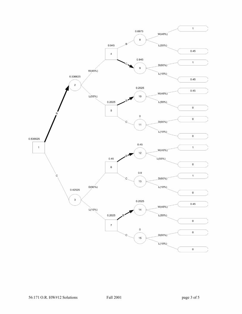
56:171 O.R. HW#12 Solutions Fall 2001 page 3 of 5
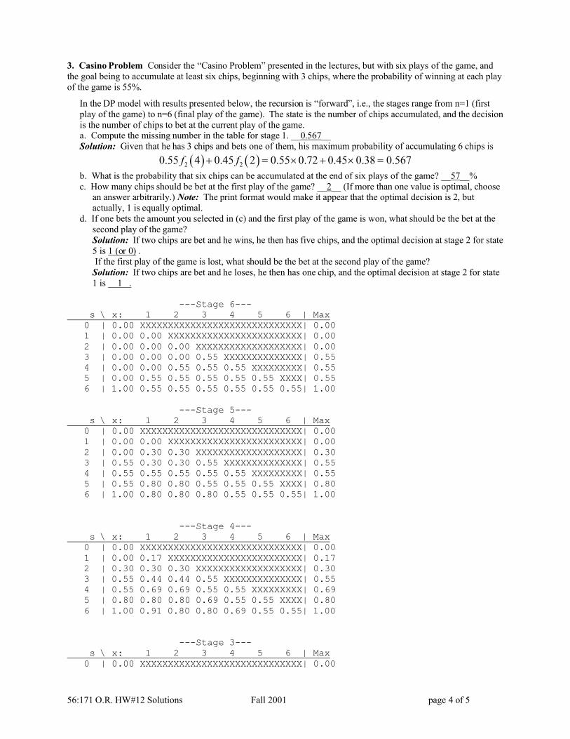
56:171 O.R. HW#12 Solutions Fall 2001 page 4 of 5
3. Casino Problem Consider the “Casino Problem” presented in the lectures, but with six plays of the game, andthe goal being to accumulate at least six chips, beginning with 3 chips, where the probability of winning at each playof the game is 55%.
In the DP model with results presented below, the recursion is “forward”, i.e., the stages range from n=1 (firstplay of the game) to n=6 (final play of the game). The state is the number of chips accumulated, and the decisionis the number of chips to bet at the current play of the game.a. Compute the missing number in the table for stage 1. __0.567__Solution: Given that he has 3 chips and bets one of them, his maximum probability of accumulating 6 chips is
( ) ( )2 20.55 4 0.45 2 0.55 0.72 0.45 0.38 0.567f f+ = × + × =b. What is the probability that six chips can be accumulated at the end of six plays of the game? __57__%c. How many chips should be bet at the first play of the game? __2__ (If more than one value is optimal, choose
an answer arbitrarily.) Note: The print format would make it appear that the optimal decision is 2, butactually, 1 is equally optimal.
d. If one bets the amount you selected in (c) and the first play of the game is won, what should be the bet at thesecond play of the game?Solution: If two chips are bet and he wins, he then has five chips, and the optimal decision at stage 2 for state5 is 1 (or 0) .If the first play of the game is lost, what should be the bet at the second play of the game?
Solution: If two chips are bet and he loses, he then has one chip, and the optimal decision at stage 2 for state1 is 1 .
---Stage 6---s \ x: 1 2 3 4 5 6 | Max0 | 0.00 XXXXXXXXXXXXXXXXXXXXXXXXXXXXX| 0.00 1 | 0.00 0.00 XXXXXXXXXXXXXXXXXXXXXXXX| 0.00 2 | 0.00 0.00 0.00 XXXXXXXXXXXXXXXXXXX| 0.00 3 | 0.00 0.00 0.00 0.55 XXXXXXXXXXXXXX| 0.55 4 | 0.00 0.00 0.55 0.55 0.55 XXXXXXXXX| 0.55 5 | 0.00 0.55 0.55 0.55 0.55 0.55 XXXX| 0.55 6 | 1.00 0.55 0.55 0.55 0.55 0.55 0.55| 1.00
---Stage 5---s \ x: 1 2 3 4 5 6 | Max0 | 0.00 XXXXXXXXXXXXXXXXXXXXXXXXXXXXX| 0.00 1 | 0.00 0.00 XXXXXXXXXXXXXXXXXXXXXXXX| 0.00 2 | 0.00 0.30 0.30 XXXXXXXXXXXXXXXXXXX| 0.30 3 | 0.55 0.30 0.30 0.55 XXXXXXXXXXXXXX| 0.55 4 | 0.55 0.55 0.55 0.55 0.55 XXXXXXXXX| 0.55 5 | 0.55 0.80 0.80 0.55 0.55 0.55 XXXX| 0.80 6 | 1.00 0.80 0.80 0.80 0.55 0.55 0.55| 1.00
---Stage 4---s \ x: 1 2 3 4 5 6 | Max0 | 0.00 XXXXXXXXXXXXXXXXXXXXXXXXXXXXX| 0.00 1 | 0.00 0.17 XXXXXXXXXXXXXXXXXXXXXXXX| 0.17 2 | 0.30 0.30 0.30 XXXXXXXXXXXXXXXXXXX| 0.30 3 | 0.55 0.44 0.44 0.55 XXXXXXXXXXXXXX| 0.55 4 | 0.55 0.69 0.69 0.55 0.55 XXXXXXXXX| 0.69 5 | 0.80 0.80 0.80 0.69 0.55 0.55 XXXX| 0.80 6 | 1.00 0.91 0.80 0.80 0.69 0.55 0.55| 1.00
---Stage 3---s \ x: 1 2 3 4 5 6 | Max0 | 0.00 XXXXXXXXXXXXXXXXXXXXXXXXXXXXX| 0.00

56:171 O.R. HW#12 Solutions Fall 2001 page 5 of 5
1 | 0.17 0.17 XXXXXXXXXXXXXXXXXXXXXXXX| 0.17 2 | 0.30 0.38 0.38 XXXXXXXXXXXXXXXXXXX| 0.38 3 | 0.55 0.51 0.51 0.55 XXXXXXXXXXXXXX| 0.55 4 | 0.69 0.69 0.69 0.62 0.55 XXXXXXXXX| 0.69 5 | 0.80 0.86 0.80 0.69 0.62 0.55 XXXX| 0.86 6 | 1.00 0.91 0.86 0.80 0.69 0.62 0.55| 1.00
---Stage 2---s \ x:0 1 2 3 4 5 6 | Max0 | 0.00 XXXXXXXXXXXXXXXXXXXXXXXXXXXXX| 0.00 1 | 0.17 0.21 XXXXXXXXXXXXXXXXXXXXXXXX| 0.21 2 | 0.38 0.38 0.38 XXXXXXXXXXXXXXXXXXX| 0.38 3 | 0.55 0.55 0.55 0.55 XXXXXXXXXXXXXX| 0.55 4 | 0.69 0.72 0.72 0.62 0.55 XXXXXXXXX| 0.72 5 | 0.86 0.86 0.80 0.72 0.62 0.55 XXXX| 0.86 6 | 1.00 0.94 0.86 0.80 0.72 0.62 0.55| 1.00
---Stage 1---s \ x: 0 1 2 3 | Max3 | 0.55 0.57 0.55 | 0.57