Center for

Mathematical Economics

Working Papers 557May 2016

Hypothesis Testing Equilibrium in Signaling

Games

Lan Sun

Center for Mathematical Economics (IMW)Bielefeld UniversityUniversitatsstraße 25D-33615 Bielefeld · Germany

e-mail: imw@uni-bielefeld.dehttp://www.imw.uni-bielefeld.de/wp/

ISSN: 0931-6558

Hypothesis Testing Equilibrium in Signaling

Games

Lan Sun∗

Center for Mathematical Economics

Bielefeld University

Version: 23. May. 2016

Abstract

In this paper, we propose a definition of Hypothesis Testing Equi-

librium (HTE) for general signaling games with non-Bayesian players

nested by an updating rule according to Hypothesis Testing model

characterized by Ortoleva (2012). An HTE may be different from

a sequential Nash equilibrium because of the dynamic inconsistency.

However, when player 2 only takes zero-probability message as an un-

expected news, an HTE is a refinement of sequential Nash equilibrium

and it survives Intuitive Criterion, but not vice versa. We provide exis-

tence theorem covering a broad class of signaling games often studied

in economics, and the constrained HTE is unique in such signaling

games. Keywords: Signaling Games, Hypothesis Testing Equilibrium,

Equilibrium Refinement.

∗Tel: +49 521 106 4923.

E-mail: lan.sun@uni-bielefeld.de.

This research is granted by European Erasmus Mundus Joint Doctoral Program. I would

like to thank Prof. Frank Riedel, Prof. Pietro Ortoleva, Prof. Christoph Kuzmics, and

Prof. Raphael Giraud, for their insightful comments and precious advice.

1

1 Introduction

Ortoleva (2012) models an agent who does not update according to Bayes’

Rule, but would “rationally” choose a new prior among a set of priors when

her original prior assigned a small probability on an realized event. He pro-

vides axiomatic foundations for his model in the form of a Hypothesis Test-

ing representation theorem for suitably defined preferences. Both the testing

threshold and the set of priors are subjective, therefore, the agent who fol-

lows this updating rule is aware of and can anticipate her updating behavior

when formulating plans.

In details, we consider the preferences of an agent over acts F which

are functions from state space Ω to a set of consequence X. If the prefer-

ence relation is Dynamic Coherence together with other standard postulates,

then the agent’s behavior can be represented by a Hypothesis Testing model

(u, ρ, ε). According to this representation, the agent has a utility function u

over consequences; a prior over priors ρ; and a threshold ε ∈ [0, 1). She then

acts as follows: Before any information comes, she has a set of priors π ∈ Π

with probability assessment ρ over Π. She chooses πΩ with highest probabil-

ity ρ(πΩ) among all π ∈ supp(ρ) as her original prior. Then she forms her

preference as the standard expected utility maximizer. As new information

(an event) A is revealed, the agent evaluates the probability of occurrence of

the event as πΩ(A). She keeps her original prior πΩ and proceeds Bayesian

update πΩ using A if the event A is not unexpected, i.e., πΩ(A) > ε. How-

ever, if πΩ(A) ≤ ε, she doubts her original prior πΩ and looks for a new prior

π∗ among supp(ρ) such that π∗ is the most likely one conditional on event

A, that is, π∗ = argmaxπ∈supp(ρ)

P(π|A), where

P(π|A) =P(A|π)P(π)∫

π′∈supp(ρ)P(A|π′)P(π′)dπ′

=π(A)ρ(π)∫

π′∈supp(ρ)π′(A)ρ(π′)dπ′

.

(1)

Using this π∗, she proceeds Bayesian update and forms her preference by

2

maximizing expected utility.

Ortoleva (2012) applied his model in the “Beer-Quiche” game and defined

a Hypothesis Testing Equilibrium (HTE) when ε = 0 for this specific game.

In this game, there exists unique HTE which coincides with the selection of

the Intuitive Criterion of Cho and Kreps (1987). This paper develops the

idea of nesting the updating model in general signaling games with finite

states and proposes a general concept of Hypothesis Testing Equilibrium.

For the general definition of HTE, we allow the testing threshold ε ≥ 0. If

player 2 has a testing threshold ε > 0, then she changes her beliefs when a

small (but non-zero) probability event happens. This dynamic inconsistency

leads to a result that an HTE may deviate from sequential Nash equilibrium.

However, we show that when ε = 0, an HTE is a refinement of sequential

Nash equilibria. In this case, player 2 only considers the zero-probability

event as an unexpected event. In order to compare with other refinement

criteria, we mainly focus on the properties of this class of HTE. We have three

main findings: (a). As a method of refinement, an HTE survives Intuitive

Criterion, but not vice verse; (b). A general HTE exists in a broad class

of signaling games studied in economics which satisfy the Single Crossing

Property together with other standard assumptions. (c). We proposed a

concept of constrained HTE in which the set of alternative beliefs of player

2 is restricted to be around her original belief. We show that the constrained

HTE is unique under the previous assumptions. As an example, we present

this result in Milgrom-Roberts’ limit pricing model and we get a unique HTE

for each interesting case.

This paper focuses on the signaling games, a class of games where an in-

formed player (player 1) conveys private information to an uninformed player

(player 2) through messages, and player 2 tries to make inferences about hid-

den information and takes an action which can influence both players’ payoffs.

There is an enormous literature that analyzes and utilizes signaling games

in applications of a wide range of economic problems as reviewed in Riley

(2001) and Sobel (2007), see Spence’s model in labor market (Spence, 1974),

3

Milgrom-Roberts’ model of limit pricing (Milgrom and Roberts, 1982), bar-

gaining models (Fudenberg and Tirole, 1983 ), and models in finance (Leland

and Pyle, 1977), for example. Typically, signaling games give rise to many

sequential Nash equilibria because under the assumption of Bayesian updat-

ing rule, at equilibrium, there is no other restrictions on the message m that

is sent with zero probability by player 1 except that player 2’s responses to

m can be rationalized by some belief of player 2. Therefore, the natural idea

to refine the sequential Nash equilibria is to impose additional restrictions

on the out-of-equilibrium beliefs as we can see in the literature reviewed in

Govindan and Wilson (2008, 2009), Hillas and Kohlberg (2002), Kohlberg

(1990), and van Damme (2002).

One branch of the refinement criteria, which has been widely applied in

signaling games in order to reduce the set of sequential equilibria, is motivated

by the concept of strategic stability for finite games addressed by Kohlberg

and Mertens (1986). The Intuitive Criterion, D1, D2 Criteria (Cho and

Kreps, 1987), Divinity (Banks and Sobel, 1987), for example, are all weaker

versions of strategic stability that are defined more easily for signaling games.

These refinements interpret the meaning of the out-of-equilibrium messages

depending on the current equilibrium, which means that, at a reasonable

equilibrium, sending an out-of-equilibrium message is costly and unattrac-

tive to player 1. There is also a branch of refinements trying to define a

new concept of equilibrium, for example, perfect sequential equilibria pro-

posed by Grossman and Perry (1986), different versions of Perfect Bayesian

Equilibrium (PBE) discussed by Fudenburg and Tirole (1991), and forward

induction equilibrium defined by Govindan and Wilsons (2009) and modified

by Man (2012), Consistent Forward Induction Equilibrium Path proposed

by Umbauer (1991), etc. There is also a few refinements that are base on

the idea of hypothesis test, see Mailath, Okuno-Fujiwara, and Postlewaite

(1993) and Ortoleva (2012), for example. There is no consensus in the liter-

ature that one refinement is better than the other. One refinement can be

favorable in some settings and unfavorable in other settings.

4

All these refinements mentioned above are dealing with signaling games

with Bayesian players. However, the behavior of deviation from Bayesian

updating has been observed by psychologists1 and these experiments mo-

tivated a growing interest in properties of non-Bayesian updating, see, for

example, the model of temptation and self-control proposed by Gul and Pe-

sendorfer (2001, 2004), characterized axiomatically by Epstein (2006), and

extended by Epstein et al., (2008, 2010), models of learning in social net-

works by Golub and Jackson (2010) and Jadbabaie et al., (2012), arguments

of rational beliefs by Gilboa et. al, (2008, 2009, 2012) and Teng (2014), and

hypothesis testing model of Ortoleva (2012), etc. For signaling games with

non-Bayesian players, this paper proposes a concept of Hypothesis Testing

equilibrium, and provides a refinement based on the idea of non-Bayesian re-

actions to small probability messages according to Hypothesis Testing model.

The non-Bayesian updating rule is nested in the signaling games as follows:

Before player 1 moves, player 2 has a prior over a (finite) set of strategies

that player 1 may use and she chooses the most likely strategy that player 1

would use. After she observes a message sent by player 1, she evaluates the

probability of the message using her original belief induced by the strategy

of player 1. She keeps her original belief and uses it to proceed Bayesian

update if the probability of the massage she observed is greater than her

testing threshold. However, if the probability is less than or equals to the

threshold, she will discard her original belief (she thinks that player 1 may

use a different strategy from her original conjecture), then she looks for a

new belief which can be induced by another “rational” strategy of player 1

such that it is the most likely one conditional on the observed message. If

there exist such beliefs to support the occurrence of the messages (for both

on-the-equilibrium path and off-the-equilibrium path massages), then the se-

quentially rational strategies profile form an HTE. The difficulty is that how

player 2 selects the set of strategies of player 1 (which can induce a set of

1For example Tversky and Kahneman (1974), Camerer (1995), Rabin (1998, 2002),

and Mullainathan (2000).

5

beliefs of player 2) and how to assign probability distribution over these pos-

sible strategies. Here we allow all the beliefs which can be “rationalized”

by at least one strategy of player 2 under consideration, which is a weak

restriction on the beliefs available to player 2.

This paper is organized as follows. In the next section, we briefly recall

the basic concepts and definitions from Ortoleva (2012) on the updating rule

of Hypothesis Testing model and the framework of general signaling games.

Section 3 is the heart of the paper, where we define the general Hypothesis

Testing Equilibrium (HTE), discuss the main properties of HTE and prove

the existence and uniqueness theorem. Section 4 compares the refinements

of HTE and Intuitive Criterion. Section 5 analyzes the HTE of Milgrom-

Roberts’ limit pricing model in a finite framework and section 6 provides the

conclusion and remarks.

2 Formulations and Preliminaries

2.1 The updating rule of Hypothesis Testing Model

Firstly we recall the basic concepts, definitions and main results of Hypoth-

esis Testing Model in general decision theory. Adopting the notations in

Ortoleva (2012), consider such a probability space (Ω,Σ,∆(Ω)), where Ω is

finite (nonempty) state space, Σ is set of all subsets of Ω, and ∆(Ω) is the

set of all probability measures (beliefs) on Ω. Write ∆(∆(Ω)) as the set of

all beliefs over beliefs. Let

BU(π,A)(B) =π(A ∩B)

π(A)

denote the Bayesian update of π ∈ ∆(Ω) using A ∈ Σ such that π(A) > 0.

As we discussed in the introduction, equation (1) gives the Bayesian update

of the second order prior ρ ∈ ∆(∆(Ω)) using A ∈ Σ such that π(A) > 0 for

6

some π ∈ supp(ρ). We denote it as:

BU(ρ,A)(π) :=π(A)ρ(π)∫

∆(Ω)

π′(A)ρ(π′)dπ′.

Let’s consider the preferences of an agent over acts F which are functions

from state space Ω to a set of consequence X. For example, X could be a

set of possible prizes depending on the realizations of the state.

Definition 2.1. (Ortoleva, 2012) A class of preferences relations AA∈Σ

admits a Hypothesis Testing Representation if there exists a nonconstant

affine function u : X → R, a prior over priors ρ ∈ ∆(∆(Ω)) with finite

support, and ε ∈ [0, 1) such that, for any A ∈ Σ, there exist πA ∈ ∆(Ω) such

that:

(i) for any f, g ∈ F

f A g ⇔∑ω∈Ω

πA(ω)u(f(ω)) ≥∑ω∈Ω

πA(ω)u(g(ω))

(ii) πΩ = argmaxπ∈∆(Ω)

ρ(π)

(iii)

πA =

BU(πΩ, A) πΩ(A) > ε

BU(π∗A, A) otherwise,

where π∗A = argmaxπ∈∆(Ω)

BU(ρ,A)(π).

Under this definition, if a decision maker’s preference is represented by

the updating rule according to Hypothesis Testing Model, then she proceeds

the update in the following procedure:

Step 0. The agent is uncertain about some important state of the nature.

Instead of a single subjective probability distribution over the alternative

possibilities, she has a set of probability distributions (priors) Π and a prob-

ability distribution (second order prior) ρ on Π, and supp(ρ) 6= ∅. The agent

has a subjective threshold ε for Hypothesis Test.

7

Step 1. Before any new information is revealed, the agent chooses a prior

πΩ ∈ supp(ρ) which is the most likely prior according to her belief ρ. In

this hypothesis test, πΩ serves as a null hypothesis and all the other priors

π ∈ supp(ρ) as alternative hypothesis.

Step 2. As new information (an event) A is revealed, the agent evaluates

the probability of the occurrence of A as πΩ(A). The null hypothesis will

not be rejected if πΩ(A) > ε, and the agent can proceed Bayes’ rule to the

prior πΩ. However, the null hypothesis will be rejected if πΩ(A) ≤ ε. The

agent doubts her original prior πΩ because an unexpected event occurred.

The agent will choose an alternative prior π∗ ∈ supp(ρ) which is the most

likely one conditional on the event A. Then she proceeds Bayes’ rule to the

prior π∗.

This paper aims to nest the non-Bayesian updating rule according to the

Hypothesis Testing model into signaling games, therefore, we now briefly

introduce the general framework of signaling games with Bayesian players

first.

2.2 Signaling Games

Nature selects the type of player 1 according to some probability distribution

µ over a finite set T with supp(µ) 6= ∅ (For simplicity, we take T = supp(µ)).

Player 1 is informed of his type t ∈ T but player 2 is not. After player 1 learnt

his type, he chooses to send a message m from a finite set M . Observing the

message m, player 2 updates his beliefs on the type of player 1 and makes

a response r in a finite action set R. The game ends with this response and

payoffs are made to the two players. The payoff to player i, i = 1, 2, is given

by a function ui : T ×M × R → R. The distribution µ and the description

of the game are common knowledge.

8

2.2.1 Sequencial Nash Equilibrium

A behavioral strategy of player 1 is a function σ : T → ∆(M) such that∑m∈M σ(m; t) = 1 for all t ∈ T . The type t of player 1 chooses to send

message m with probability σ(m; t) for all t ∈ T . A behavioral strategy of

player 2 is a function τ : M → ∆(R) such that∑

r∈R τ(r;m) = 1 for all

m ∈ M . Player 2 takes respond r following the message m with probability

τ(r;m). We adopt the notations in Cho and Kreps (1978), write BR(m,µ)

for the set of best responses of player 2 observing m if she has posterior belief

µ(·|m).

BR(m,µ) = argmaxr∈R

∑t∈T

u2(t,m, r)µ(t|m).

If T ′ ⊆ T , let BR(T ′,m) denote the set of best responses of player 2 to

posteriors concentrated on the set T ′. That is,

BR(T ′,m) =⋃

µ:µ(T ′|m)=1

BR(m,µ).

Let BR(T ′,m, µ) be the set of best responses by player 2 after observing m

if she has posterior belief µ(·|m) concentrated on the subset T ′, and MBR

denote the set of mixed best responses by player 2. Since we concentrate

on the finite sets of T , M , and R, the sequential Nash equilibrium can be

defined straightforward.

Proposition 2.1. A profile of players’ behavioral strategies (σ∗, τ ∗) forms

a sequential Nash equilibrium (SNE) in a finite signaling game if it satisfies

the following conditions:

(i) Given player 2’s strategy τ ∗, each type t evaluates the expected utility

from sending message m as∑

r∈R u1(t,m, r)τ ∗(r;m) and σ∗(·; t) puts weight

on m only if it is among the maximizing m’s in this expected utility.

(ii) Given player 1’s strategy σ∗, for all m that are sent by some type t with

positive probability µ(t|m) > 0 , every response r ∈ R such that τ ∗(r;m) > 0

must be a best response to m given beliefs µ(t|m), that is,

τ ∗(·;m) ∈ MBR(m,µ(·|m)), (2)

9

where µ(t|m) = σ∗(m;t)µ(t)∑t′∈T σ

∗(m;t′)µ(t′).

(iii) For every message m that is sent with zero probability by player 1

(for all m such that∑

t σ∗(m; t)µ(t) = 0), there must be some probability

distribution µ(·|m) over types T such that (2) holds.

In an SNE, given the strategy of player 1, player 2 proceeds three steps:

she computes the probability of an observed messagem as P(m) =∑

t∈T σ∗(m; t)µ(t).

If P(m) > 0, that is, there exists some t ∈ T , such that σ∗(m; t) > 0, then

she uses Bayes’ rule to compute the posterior assessment µ(·|m), and then

she chooses her best response to m compatible with her belief µ(·|m). If

P(m) = 0, then there only needs to exist some belief µ(·|m) such that her

responses to the out-of-equilibrium message is rational.

What happens if player 2 is a non-Bayesian player? In the next section, we

aim to define an alternative equilibrium in such signaling games where player

2 uses non-Bayesian update rule according to Hypothesis Testing model.

3 Hypothesis Testing Equilibrium

3.1 Definition of HTE in general signaling games

In a signaling game, player 2 does not observe player 1’s strategies but the

messages sent by player 1, therefore, it’s helpful to imagine that player 2 has

a conjecture, σ(·; t), ∀t ∈ T , about player 1’s behavior. She attempts to make

inference using her conjecture. Similarly, player 1 also has a conjecture, τ ,

about player 2’s behavior and, at equilibrium, the conjectures (σ, τ) coincide

with the strategies (σ∗, τ ∗) that players actually use. Each one conjecture σ

of player 2 about player 1’s behavior induces a prior (belief) π on the state

space Ω = T ×M . For every realization (t,m), π(t,m) is the probability of

type t sending message m which is

π(t,m) = σ(m; t)µ(t),

10

and satisfies ∑t∈T

∑m∈M

π(t,m) =∑t

µ(t) = 1.

If player 2 is non-Bayesian player and her preference is represented by the

Hypothesis Testing model, then player 2 has a set of “rational” conjectures

(priors) and she has a probability distribution ρ on the set of conjectures

(priors). Firstly, we address some proper requirements for the second order

prior ρ.

Definition 3.1. Consider a finite signaling game Γ(µ) where player 2’s pref-

erence is represented by a Hypothesis Testing model (ρ, ε). ρ is consistent if

it satisfies the following requirements:

(i). ∀π ∈ supp(ρ), π is compatible with the initial information of the

game, that is∑

m∈M π(t,m) = µ(t).

(ii). ∀π ∈ supp(ρ), π can be rationalized by at least one possible strategy

of player 2. that is, there exists some strategy τ : M → ∆(R) of player 2

such that π(t,m) = 0,∀t ∈ T,∀m ∈M , if the type-message pair (t,m) is not

a best response to τ .

As addressed in Ortoleva (2012), the requirement for rationality is a weak

condition in the sense that player 2 can take any conjecture under consid-

eration as long as it is compatible with player 1’s best responding to some

possible strategy τ of player 2. Now we are ready to define Hypothesis Test-

ing Equilibrium in signaling games.

Definition 3.2. In a finite signaling game Γ(µ), a profile of behavioral strate-

gies (σ∗, τ ∗) is a Hypothesis Testing equilibrium (HTE) based on a Hypothesis

Testing model (ρ, ε) if

(i). ρ is consistent.

(ii). The support of ρ contains πΩ induced by σ∗ such that

πΩ = argmaxπ∈supp(ρ)

ρ(π).

11

Let

ME = m ∈M :∑t∈T

πΩ(m|t)µ(t) > ε,

then for any m ∈M\ME, there exists some πm ∈ supp(ρ), such that

πm = argmaxπ∈supp(ρ)

BU(ρ,m)(π).

(iii).For all t ∈ T , σ∗(m; t) > 0 implies m maximizes the expected utility

of player 1, that is∑r∈R

u1(t,m, r)τ ∗(r;m). ∀m ∈M ,

τ ∗(·;m) ∈ MBR(m,µ(·|m)),

where

µ(t|m) =

πΩ(t|m) = σ∗(m;t)µ(t)∑t′ σ∗(m;t′)µ(t′)

if m ∈ME

πm(t|m) = πm(m|t)µ(t)∑t′ πm(m|t′)µ(t′)

, otherwise.

The idea behind this definition is similar as Nash equilibrium except that

we allow non-Bayesian reactions for out-of-equilibrium messages when ε > 0.

Therefore, the dynamic consistency is violated but only up to ε. However,

the dynamic consistency holds when ε = 0 and the update rule is also well

defined after zero-probability messages. According to the definition, for a

given ε, in order to prove a profile of strategies is an HTE based on (ρ, ε), we

just need to find a proper ρ to support the equilibrium.

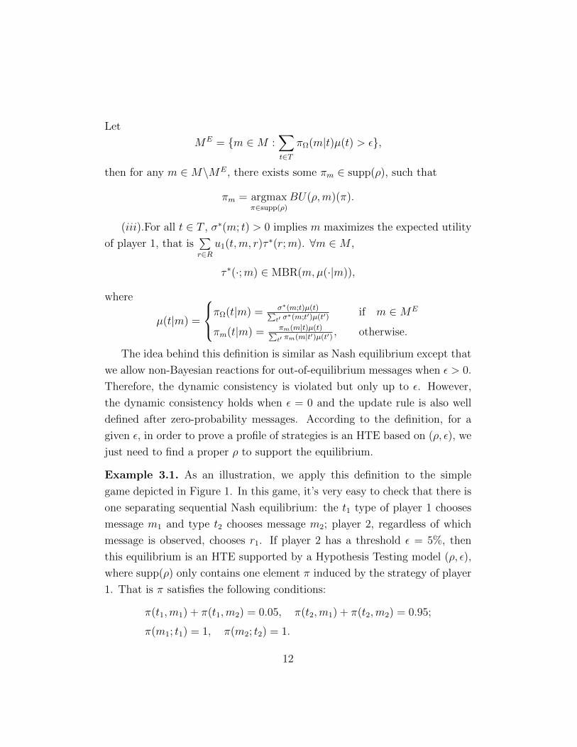
Example 3.1. As an illustration, we apply this definition to the simple

game depicted in Figure 1. In this game, it’s very easy to check that there is

one separating sequential Nash equilibrium: the t1 type of player 1 chooses

message m1 and type t2 chooses message m2; player 2, regardless of which

message is observed, chooses r1. If player 2 has a threshold ε = 5%, then

this equilibrium is an HTE supported by a Hypothesis Testing model (ρ, ε),

where supp(ρ) only contains one element π induced by the strategy of player

1. That is π satisfies the following conditions:

π(t1,m1) + π(t1,m2) = 0.05, π(t2,m1) + π(t2,m2) = 0.95;

π(m1; t1) = 1, π(m2; t2) = 1.

12

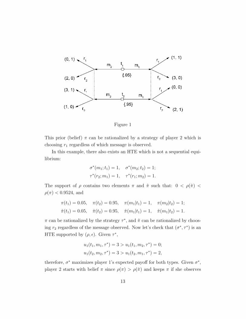
Figure 1

This prior (belief) π can be rationalized by a strategy of player 2 which is

choosing r1 regardless of which message is observed.

In this example, there also exists an HTE which is not a sequential equi-

librium:

σ∗(m1; t1) = 1, σ∗(m2; t2) = 1;

τ ∗(r2;m1) = 1, τ ∗(r1;m2) = 1.

The support of ρ contains two elements π and π such that: 0 < ρ(π) <

ρ(π) < 0.9524, and

π(t1) = 0.05, π(t2) = 0.95, π(m1|t1) = 1, π(m2|t2) = 1;

π(t1) = 0.05, π(t2) = 0.95, π(m1|t1) = 1, π(m1|t2) = 1.

π can be rationalized by the strategy τ ∗, and π can be rationalized by choos-

ing r2 regardless of the message observed. Now let’s check that (σ∗, τ ∗) is an

HTE supported by (ρ, ε). Given τ ∗,

u1(t1,m1, τ∗) = 3 > u1(t1,m2, τ

∗) = 0;

u1(t2,m2, τ∗) = 3 > u1(t2,m1, τ

∗) = 2,

therefore, σ∗ maximizes player 1’s expected payoff for both types. Given σ∗,

player 2 starts with belief π since ρ(π) > ρ(π) and keeps π if she observes

13

m2 since

π(m2) = π(m2|t1)π(t1) + π(m2|t2)π(t2) = 0.95 > ε.

With the posterior belief π(·|m2), observing m2, player 2’s best response is

r1. She switches to belief π if she observes m1 since

π(m1) = π(m1|t1)π(t1) + π(m1|t2)π(t2) = 0.05 ≤ ε,

and

BU(ρ,m1)(π) > BU(ρ,m1)(π).

Therefore, observing m1, player 2 has the posterior assessments of π(t1|m1) =

0.05 and π(t2|m1) = 0.95. With this posterior belief, player 2 computes her

expected payoffs as:

u2(r1;m1, σ∗) = π(t1|m1)× 1 + π(t2|m1)× 0 = 0.05;

u2(r2;m1, σ∗) = π(t1|m1)× 0 + π(t2|m1)× 1 = 0.95,

which implies that r2 is the best response to m1. Therefore, (σ∗, τ ∗) is an

HTE but it’s not a Nash Equilibrium, since r2 is not a best response of player

2 to the message m1 if she only has one belief π.

3.2 Properties of Hypothesis Testing Equilibrium

From the previous example, we can immediately get the following property:

Proposition 3.1. In a finite signaling game Γ(µ), if a profile of behavioral

strategies (σ, τ) is an HTE supported by a Hypothesis Testing model (ρ, 0),

then it’s also an HTE supported by a Hypothesis Testing model (ρε, ε), for all

ε > 0.

Proof. Let ME0 and ME

ε denote the sets of messages which are sent with

zero probability by player 1 and less than or equal to ε, respectively. Then

MEε ⊆ME

0 . We can simply take

ρε = ρ = πΩ, πm,m ∈M\ME.

14

Player 2 starts with πΩ = argmaxπ∈supp(ρ) ρ(π), he keeps πΩ and proceeds

Bayesian update if she observed m ∈ MEε . If m ∈ ME

0 \MEε , there exists

πm = πΩ such that σ and τ are sequentially rational. If m /∈ ME0 , there

exists π′m which is identical with πm such that σ and τ are sequentially

rational.

As we can see in the previous example, if ε > 0, then any message sent

with probability less than or equal to ε is an off-the-equilibrium message.

Because of the dynamic inconsistency, an HTE may deviate from a sequential

Nash equilibrium. However, when ε = 0, only the messages sent with zero-

probability are off-the-equilibrium path, therefore, it is not surprising that

there is a close relationship between this special class of HTE and sequential

Nash equilibrium.

Proposition 3.2. In a finite signaling game Γ(µ), an HTE supported by a

Hypothesis Testing model (ρ, 0) is a refinement of SNE.

This requires no proof, it’s just a matter of definitions of HTE and SNE.

If a profile of strategies (σ∗, τ ∗) is an HTE supported by (ρ, 0), then for any

message sent by player 1 such that σ∗(m; t) > 0 for some t ∈ T , player 2’s

posterior belief derived by Bayesian update using σ∗. And for any message

sent with zero probability, that is, σ∗(m; t) = 0 for all t ∈ T , there exists

some belief on the side of player 2 to rationalize her behavior. In addition,

(σ∗, τ ∗) are sequentially rational. Therefore, (σ∗, τ ∗) is an SNE.

On the other side, according to definition 3.2, we require that any belief in

the support of ρ must can be “rationalized” by at least one strategy of player

2, which means, in addition to the requirement of equation (2), we impose

a further restriction on the off-the-equilibrium beliefs of player 2, therefore,

it’s not surprise that an SNE may not be an HTE supported by some (ρ, 0)

as the “Quiche-Beer” game in Ortoleva (2012). Here we also give a simple

example2 to show this property.

2This example is from Cho and Kreps (1987)

15

200 QUARTERLY JOURNAL OF ECONOMICS

0~~~ 1.1 1 r2 (r) m t2 ~ ,M(

(o) ~~1 r2 (-)

FIGURE III

the m' information set must put weight 0.5 or more on A being type t2. But for type t2, m dominates m'. So, by any of the tests constructed from the dominance criterion above, we can prune the type-message pair (t2,m') from the game. In the game that is left, B must respond to m' with r2. This causes the equilibrium outcome to fail the test, using either Step 2 or 2A, since this response causes t1 to defect.

The game in normal form is given in Table I. (Note that the prior enters into the expected payoff calculations.) We leave to the reader the simple task of verifying that the equilibrium in which A chooses m regardless of type and B responds to m' with r1 is indeed proper. (Moreover, it is easily shown to be perfect in the agent normal form.)

This example can be used to make another point, concerning properness for signaling games. (The material in this paragraph is a bit esoteric, and it may be skipped without loss of comprehension of most of the rest of the paper.) Consider changing the prior on A's type, from 0.9 that A is t1 to 0.9 that A is t2. Since, to support the m equilibrium outcome, it is necessary that B "assess" high posterior

TABLE I GAME OF FIGURE III IN NORMAL FORM

Response

ri r2

Message if tl t2

m m 0,0 0,0 m m -0.1, 0.1 -0.1, 0 m' m -0.9,0 0.9, 0.9 m' m' -1, 0.1 0.8,0.9

This content downloaded from 129.70.237.97 on Mon, 21 Sep 2015 07:15:38 UTCAll use subject to JSTOR Terms and Conditions

Figure 2

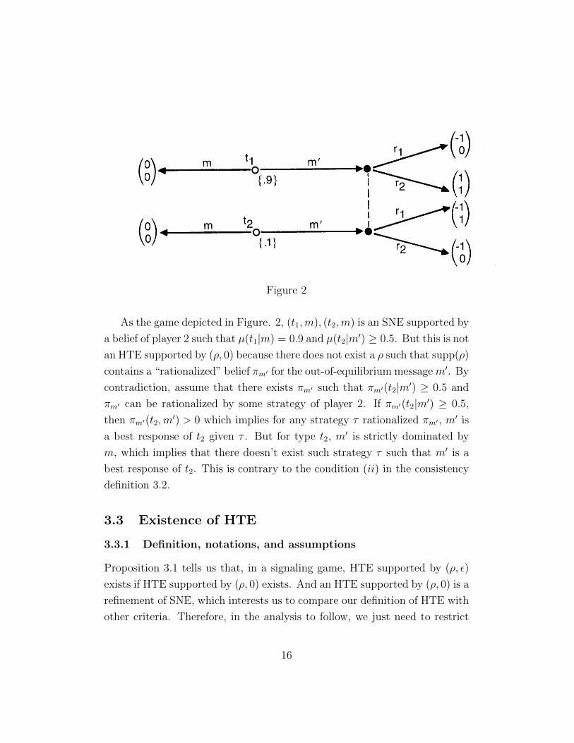
As the game depicted in Figure. 2, (t1,m), (t2,m) is an SNE supported by

a belief of player 2 such that µ(t1|m) = 0.9 and µ(t2|m′) ≥ 0.5. But this is not

an HTE supported by (ρ, 0) because there does not exist a ρ such that supp(ρ)

contains a “rationalized” belief πm′ for the out-of-equilibrium message m′. By

contradiction, assume that there exists πm′ such that πm′(t2|m′) ≥ 0.5 and

πm′ can be rationalized by some strategy of player 2. If πm′(t2|m′) ≥ 0.5,

then πm′(t2,m′) > 0 which implies for any strategy τ rationalized πm′ , m

′ is

a best response of t2 given τ . But for type t2, m′ is strictly dominated by

m, which implies that there doesn’t exist such strategy τ such that m′ is a

best response of t2. This is contrary to the condition (ii) in the consistency

definition 3.2.

3.3 Existence of HTE

3.3.1 Definition, notations, and assumptions

Proposition 3.1 tells us that, in a signaling game, HTE supported by (ρ, ε)

exists if HTE supported by (ρ, 0) exists. And an HTE supported by (ρ, 0) is a

refinement of SNE, which interests us to compare our definition of HTE with

other criteria. Therefore, in the analysis to follow, we just need to restrict

16

our attention on this class of HTE imposing ε = 0. Since the mixed strategies

are not needed for the existence, we only consider the Pure Sequential Nash

Equilibrium (PSNE). A pure strategy of player 1 is a mapping s1 : T → M ,

and a pure strategy of player 2 is a response function s2;M → R.

Definition 3.3. In a finite signaling game Γ(µ), a profile of strategies (s∗1, s∗2)

forms a PSNE if there exists βm ∈ ∆(T ), ∀ m /∈ME, such that:

(i). Given s∗2,

u1(t, s∗1(t), s∗2(s∗1(t))) ≥ u1(t,m, s∗2(m)), ∀m ∈M, ∀t ∈ T,

(ii).Given s∗1, for any m ∈M , s∗2(m) ∈ BR(m,µ2(·|m)), where

µ2(t|m) =

β(t|m) if m ∈ME

βm(t|m) otherwise,

and

β(t|m) =

µ(t)∑

t′∈Tm,s∗1µ(t′)

if t ∈ Tm,s∗1

0, otherwise,

where Tm,s∗1 = t ∈ T : s∗1(t) = m.

Before we go to the prove of existence, we provide some notations that

we may use in the statements.

Tm,s1 : the subset of types of player 1 who send message m under strategy s1,

that is,

Tm,s1 = t ∈ T : s1(t) = m.

ME(s1,s2): the set of on-the-equilibrium messages if (s1, s2) ∈ PSNE(Γ(µ)),

that is,

ME(s1,s2) = m ∈M : ∃t ∈ T, s.t.s1(t) = m.

u1(t; s1, s2): the payoff of type t under strategy (s1, s2), that is,

u1(t; s1, s2) = u1(t, s1(t), s2(s1(t))).

17

βTm ∈ ∆(T ): the probability assessment concentrating on types t ∈ Tm, that

is,

βTm(t) =

µ(t)∑

t′∈Tm µ(t′)if t ∈ Tm

0 otherwise.

βt ∈ ∆(T ): the probability assessment concentrating on type t, that is,

βt(t′) =

1 if t′ = t

0 otherwise

We cannot be confident that there exists an HTE for a game that is

randomly selected from the space of signaling games with finite states, we

prove the existence theorem in the class of signaling games that satisfy the

following assumptions.

Assumption 1. T , M , and R are finite. The type of player 1 has a probabil-

ity distribution, µ ∈ ∆(T ), with full support. Further, ui(t, s1, s2) , i ∈ 1, 2,exists and is finite for all t ∈ T and all nondecreasing functions s1 : T →M

and s2 : M → R.

Assumption 2. For any t ∈ T , for any fixed r ∈ R, if we connect the points

u1(t,m, r) : m ∈M in order by a smooth line, then u1(t) is strictly concave

in m, and u2 is strictly concave in r.

Assumption 3. First order stochastic dominance: ∀t ∈ T , ∀m ∈ M ,

∀β, β′ ∈ ∆(T ), whenever β stochastically dominants β′, that is∑t′≤t

β′(t′) ≥∑t′≤t

β(t′), ∀t ∈ T,

and strictly inequality holds for some t ∈ T , then

u1(t,m,BR(m,β)) > u1(t,m,BR(m,β′)).

18

Assumption 4. Single Crossing Property:

(i). For all m > m′, and all t′ > t,∀r, r′ ∈ R,

u1(t,m, r) ≥ (>)u1(t,m′, r′), implies

u1(t′,m, r) ≥ (>)u1(t′,m′, r′).

(ii). For all r > r, and all m > m, ∀ t ∈ T ,

u2(t,m, r) ≥ (>)u2(t,m, r), implies

u2(t, m, r) ≥ (>)u2(t, m, r).

Assumption 1 is primarily a technical assumption to fit our definition of

HTE. Assumption 2 insures that only pure strategies are under consideration

for both players. Assumption 3 says that all types of player 1 prefer the best

response of player 2 when player 2 believes that player 1 is more likely to be

a higher type. The forth assumption is the Milgrom-Shannon single crossing

property (SCP) for both players, which is a widely used assumption in the

signaling games to model many economic problems. It says that if type t

prefers a higher message-response pair (m, r) to a lower message-response

pair (m′, r′), then any higher type t′ > t also prefers the higher message-

response pair (m, r). This captures the idea that higher messages are easier

to send by a higher type. The utility of player 2 also satisfies SCP: if r is a

better response to a message m sent by type t than r, then it is also a better

response to a higher message m sent by t than r.

Before we proceed the existence theorem, let us review the concept of

lexicographically dominance introduced by Mailath. et, al., (1993).

Definition 3.4. In a signaling game Γ(µ), a strategy profile (s∗1, s∗2) ∈

PSNE(Γ(µ)) lexicographically dominates (l -dominates) another strategy pro-

file (s1, s2) ∈ PSNE(Γ(µ)) if there exists j ∈ T , such that

u1(t; s∗1, s∗2) > u1(t; s1, s2) if t = j

u1(t; s∗1, s∗2) ≥ u1(t; s1, s2) if t ≥ j + 1.

19

A strategy profile (s∗1, s∗2) ∈ PSNE(Γ(µ)) is a lexicographically maximum se-

quential equilibrium (LMSE) if there doesn’t exist an (s1, s2) ∈ PSNE(Γ(µ))

l -dominates (s∗1, s∗2).

If we restrict player 1’s types in a subset of T , we can define a truncated

game from G. Formally, for any j ∈ T , let

T j = 1, ..., j, µj(t) = βT j .

A truncated gameGj is defined by substituting T j for T , and the T j−conditional

prior µj for the prior µ in original game. Then we can get the following prop-

erties:

Proposition 3.3. Assume (s1, s2) ∈ PSNE(Γ(µ)), ∀ j ∈ T , if s1(t) 6= s1(j),

∀t > j, then (sj1, sj2) ∈ PSNE(Γj(µj)), where sj1(t) = s1(t), ∀ t ≤ j, and

sj2(m) = s2(m) ∀ m ∈M .

The following lemma derived in Mailath et al (1993) is very important

in our proof. The reader is urged to read their paper to obtain a detailed

analysis of this result.

Proposition 3.4. Mailath et al (1993): Under A1-A4, suppose (s1, s2) ∈PSNE(Γ(µ)), (s1, s2) ∈ PSNE(Γj(µj)), for some j ∈ T . Suppose further that

u1(j; s1, s2) > u1(j; s1, s2),

then there exists (s∗1, s∗2) ∈ Γ(µ), such that:

u1(t; s∗1, s∗2) ≥ u1(t; s1, s2) for all t ≤ j and

u1(t; s∗1, s∗2) ≥ u1(t; s1, s2) for all t > j.

That is, (s∗1, s∗2) l-dominates (s1, s2).

3.3.2 Existence of HTE supported by a Hypothesis Testing model

(ρ, 0)

Theorem 3.5. Under A1− A4, an LMSE is an HTE.

20

In order to prove the theorem, we need the following critical results:

Lemma 3.6. (Athey, 2001): Under A1 and A4, there exists a PSNE in

Γ(µ).

Therefore, an LMSE exists. More over, both players play nondecreasing

strategies:

Lemma 3.7. Under A1 and A4, ∀ (s∗1, s∗2) ∈ PSNE(Γ(µ)), s∗1(t) ≤ s∗1(t′) if

t < t′.

Proof. At equilibrium (s∗1, s∗2) , ∀t, t′ ∈ T ,

u1(t; s∗1, s∗2) ≥ u1(t, s∗1(t′), s∗2(s∗1(t′))).

Suppose s∗1(t) > s∗1(t′) , and t′ > t, by assumption of SCP,

u1(t′; s∗1, s∗2) > u1(t′; s∗1(t′), s∗2(s∗1(t′))) = u∗1(t′; s∗1, s

∗2),

which upsets the equilibrium.

Lemma 3.8. Under A1 and A4, ∀ (s∗1, s∗2) ∈ PSNE(Γ(µ)), s∗2(m) ≤ s∗2(m′)

if m < m′.

Proof. At equilibrium (s∗1, s∗2) , ∀m′ > m ∈M , since s∗2(m) is a best response

to message m for any t,

u2(t′,m, s∗2(m)) ≥ u2(t′,m, s∗2(m′)).

Suppose s∗2(m) > s∗2(m′), from assumption A4

u2(t′,m′, s∗2(m)) ≥ u2(t′,m′, s∗2(m′)),

which is contrary to the fact that s∗2(m′) is a best response to m′.

Lemma 3.9. For an (s∗1, s∗2) ∈ PSNE(Γ(µ)), let

T (r) = t ∈ T : u1(t,m, r) > u1(t; s∗1, s∗2), (3)

then under A1 and A4, T (r) is convex.

21

Proof. For all t′, t′′ ∈ T (r), t′ < t′′, suppose ∃ t ∈ [t′, t′′], such that

u1(t,m, r) ≤ u1(t; s∗1, s∗2).

If m > s∗2(t), since t′ < t, by A4, we obtain

u1(t′,m, r) ≤ u1(t′, s∗1(t), s∗2(s∗1(t))).

And at equilibrium,

u1(t′, s∗1(t), s∗2(s∗1(t))) ≤ u1(t′; s∗1, s∗2),

therefore,

u1(t′,m, r) ≤ u1(t′; s∗1, s∗2),

which is contrary to the assumption that t′ ∈ T (r). We can analogously

prove the other case where m < s∗2(t) to get a contradiction with t′′ ∈ T (r).

Therefore, ∀ t ∈ [t′, t′′], t ∈ T (r), which implies that T (r) is convex.

Given a response r of player 2 to message m, T (r) is the set of types who

are willing to deviate from the equilibrium strategy.

Lemma 3.10. If r < r′, then T (r) ⊆ T (r′).

Proof. ∀ t ∈ T (r),

u1(t,m, r) < u1(t,m, r′)

u1(t,m, r) > u1(t; s∗1, s∗2).

The first inequality holds because of A3. Therefore

u1(t; s∗1, s∗2) < u1(t,m, r′),

which implies that t ∈ T (r′).

This lemma implies that a higher response to message m induces more

types of player 1 to deviate from the equilibrium strategy. Now let us prove

Theorem 3.5:

22

Proof. Let (s1, s2) be an LMSE in Γ(µ). In order to prove (s1, s2) is an

HTE, we just need to prove that for any out-of-equilibrium message m, there

exists a belief β(·|m) ∈ ∆(T ), such that s2(m) = BR(m,β(·|m)), can be

rationalized by some strategy s2,m : M → R. Then we can construct the

hypothesis testing model (ρ, 0) in which the support of ρ contains priors

derived from beliefs of on-the-quilibrium messages and out-of-equilibrium

messages. Suppose m is an out-of-equilibrium message. Let

Rm = r ∈ R : ∃t ∈ T, s. t. u1(t,m, r) > u1(t; s1, s2). (4)

Case (i). Rm = ∅. In this case, no type would deviate to m from his

equilibrium strategy given any response of player 2, that is, β(t|m) = 0, ∀t ∈ T . Such β can be rationalized by s2.

Case (ii). Rm 6= ∅. Due to lemma 3.8, let us consider rm = minRm, then for

all r > rm, ∃ t0 ∈ T ,

u1(t0; s1, s2) < u1(t0,m, r),

which implies that any β(·|m) ∈ ∆(T ) supporting the equilibrium (s1, s2)

must satisfy

BR(m,β(·|m)) < rm.

According to lemma 3.9, we can denote T (rm) = [i, j], where

i = mint ∈ T : u1(t,m, rm) > u1(t; s1, s2)j = maxt ∈ T : u1(t,m, rm) > u1(t; s1, s2).

We denote mj = s1(j) and k = maxt ∈ T : s1(t) = s1(j). If m > mj,

then k = j by assumption A4. If m < mj, then u(t,mj, rm) > u(t,m, rm),

for all t ∈ [j, k] because of the concavity assumption A2. Now let’s consider

the k-truncated game Γk(µk). We claim that there doesn’t exist a profile of

strategies (sk1, sk2) ∈ PSNE(Γk(µk)) such that sk1(t) = m and sk2(m) = rm for

any t ∈ [i, j]. Suppose, contrary to the assertion, there exists such equilibrium

(sk1, sk2), and at equilibrium, ∃j0 ∈ [i, j],

sk1(j0) = m, and

sk2(m) = rm.

23

We denote

h = maxt ∈ [i, k], sk1(t) = sk1(j0),

h < j because either j = k or sk1(t) > m. ∀t ∈ [j, k]. By Prop. 3.3, (sk1, sk2) is

a PSNE in h-truncated game Γh(µh) by just simply dropping the strategies

of types higher than h, and

u1(h; sk1, sk2) > u1(h; s1, s2),

therefore, Prop. 3.4 implies that there exists (s∗1, s∗2) l -dominates (s1, s2),

which is contrary to the assumption that (s1, s2) is LMSE. This analysis

means that for any (sk1, sk2) ∈ PSNE(Γk(µk)), BR(m,β[i,j]) < rm. Especially,

(s1, s2) is a PSNE of Γk(µk) by simply deleting the strategies of the types

higher than k, therefore, s2(m) < rm. To sum up the argument above, for

any out-of-equilibrium message m, for any belief β(·|m) ∈ ∆(T ), such that

s2(m) = BR(m,β(·|m)), can be rationalized by the strategy s2 of player 2:

s2(m) = rm,

s2(m′) = s2(m′), ∀m′ 6= m.

For all t ∈ T (rm),

u1(t,m, s2(m)) = u1(t,m, rm)

> u1(t; s1, s2)

≥ u1(t,m′, s2(m′)) ∀m′ ∈M= u1(t,m′, s2(m′)) ∀m′ ∈M,

and for all t /∈ T (rm), ∃ s1(t) 6= m, such that u1(t,m, s2(m)) ≤ u1(t; s1, s2).

Therefore,

β(m|t) = 1, ∀t ∈ T (rm),

β(m|t) = 0, ∀t /∈ T (rm).

We can construct a Hypothesis Testing model (ρ, 0) in which

supp(ρ) = πΩ, πm : ∀m /∈ME(s1,s2),

24

where

πΩ(·|m) = βTm,s1, ∀m ∈ME

(s1,s2)

πm(t|m) = β(t|m) = βT (rm), ∀t ∈ T, ∀m /∈ME(s1,s2),

with

ρ(πm) = 0, if m /∈ME(s1,s2) and Rm = ∅.

0 < ρ(πm) = ρ(π′m) < ρ(πΩ) if m,m′ /∈ME(s1,s2), Rm 6= ∅ and R′m 6= ∅.

By construction, (s1, s2) is an HTE supported by (ρ, 0).

3.4 Uniqueness of Constrained HTE

As we mentioned before, the condition (ii) for the requirements of consistency

of ρ is a weak condition in the sense that player 2 is allowed to take any

strategy as long as player 1 is rational to this strategy, which enlarges the set

of alternative beliefs of player 2. However, it is a natural idea if we restrict

the strategies of player 2 such that her alternative beliefs are around her

original belief.

Definition 3.5. An HTE (s1, s2) ∈ PSNE(Γ(µ)) is called constrained HTE

if for any m /∈ ME(s1,s2), and Rm 6= ∅, for any posterior belief β(·|m) ∈ ∆(T )

such that s2(m) = BR(m,β(·|m)), then β(·|m) can be rationalized by

s2(m) = rm

s2(m′) = s2(m′) ∀m′ 6= m,(5)

where rm = minRm defined in Equ. (4).

Remark 1. In a constrained HTE, any belief of an out-of-equilibrium message

supporting the equilibrium can be rationalized by a strategy of player 2 which

is not far from her equilibrium strategy. This idea is quite intuitive, when

player 2 observes a message deviated from her original belief, she looks for the

most likely types who have potential incentive to send this message and forms

her new belief through only perturbing her original belief on this message.

25

Remark 2. We notice that s2 may not be a best response to s1, only s1 is

required to be a best response to s2. If (s1, s2) forms an equilibrium, then at

this equilibrium, u1(t,m, rm) ≤ u1(t; s1, s2), ∀ t ∈ T . This case coincides with

the Consistent Forward Induction Equilibrium Path proposed by Umbhauer

(1991).

Remark 3. Go through the proof of the existence theorem, we can see that

an LMSE is a constrained HTE.

Proposition 3.11. Under A1-A4, LMSE is unique.

Proof. Suppose both (s∗1, s∗2) and (s1, s2) are LMSE, since (s∗1, s

∗2) is not l -

dominates (s1, s2), for any t0 ∈ T , such that:

u1(t0; s∗1, s∗2) > u1(t0; s1, s2),

∃t1 > t0, such that

u1(t1; s∗1, s∗2) < u1(t1; s1, s2).

We have the same expression for (s1, s2), and T is finite, therefore, (s∗1, s∗2)

and (s1, s2) are identical.

Clearly, all other strategies profile (s1, s2) ∈ PSNE(Γ(µ)) must be l -

dominated by the unique LMSE. Let us denote the unique LMSE as (sLM1 , sLM2 ),

Theorem 3.12. Under A1-A4, if the unique LMSE is complete separating,

and M is rich enough, then the outcome of constrained HTE supported by

(ρ, 0) is unique.

Lemma 3.13. Under A1-A4, assume (s1, s2) ∈ PSNE(Γ(µ)) is a completely

separating equilibrium, let j = mint ∈ T : u1(t; sLM1 , sLM2 ) > u1(t; s1, s2).If ∀ t ∈ T , s1(t) 6= sLM1 (j), then (s1, s2) is not a constrained HTE.

Proof. If j = mint ∈ T : u1(t; sLM1 , sLM2 ) > u1(t; s1, s2), We denote:

sLM1 (j) = m, sLM2 (m) = r∗j ,

s1(j) = mj, s2(mj) = rj;

26

We assume that β(·|m) ∈ ∆(T ) is a posterior belief supporting the equi-

librium (s1, s2), then R(m) 6= ∅ since u1(j,m, r∗j ) > u1(j; s1, s2). Let rm =

minRm, then r∗j ≥ rm. Further, we can show that rm = r∗j . This is true

because of the following argument: By assumption, we have can obtain that:

u1(j,m, r∗j ) > u1(j,mj, rj) and

u1(j,mj, rj) > u1(j,m, s2(m)),

⇒u1(j,m, r∗j ) > u1(j,m, s2(m))

⇒s2(m) < r∗j

⇒BR(m,β(·|m)) < BR(m,βj),

since (sLM1 , sLM2 ) is a completely separating equilibrium. Therefore,∑t∈T

β(t|m) < µ(j), and ∃t0 < j, β(t0|m) > 0.

Let

T (rm) = t ∈ T : u1(t,m, rm) > u1(t, s1, s2).

By contradiction, suppose (s1, s2) is a constrained HTE, then β(·|m) can be

rationalized by s2 given in Equ. (5). And β(t0|m) > 0 implies that m is

a best response of t0, that is, u1(t0,m, s2) > u1(t0,m′, s2(m′)), ∀ m′ ∈ M .

Therefore, t0 ∈ T (rm). However,

u1(t; sLM1 , sLM2 ) ≤ u1(t; s1, s2) ∀t < j,

which together with

u1(t; sLM1 , sLM2 ) ≥ u1(t;m, r∗j ),

implies that

u1(t,m, r∗j ) < u1(t; s1, s2) ∀t < j.

Therefore, ∀ r < r∗j ,

u1(t0,m, r) ≤ u1(t0;m, r∗j ) < u1(t0; s1, s2).

27

Therefore, rm ≥ r∗j , which induces rm = r∗j . However, with this strategy s2,

u1(j,m, s2) = u1(j,m, r∗j ) > u1(j; s1, s2) ≥ u1(j,m′, s2(m′)), ∀m′ ∈M

which implies that j ∈ Trm . Therefore, β(j|m) ≥ µ(j). We have a contradic-

tion with∑

t∈T β(t|m) < µ(j).

Now let us prove Theorem 3.12.

Proof. We just need to show that any (s1, s2) ∈ PSNE(Γ(µ)) l -dominated by

(sLM1 , sLM2 ) is not a constrained HTE. For any (s1, s2) ∈ PSNE(Γ(µ)), let

j = mint ∈ T : u1(t; sLM1 , sLM2 ) > u1(t; s1, s2),

and sLM1 (j) = mj. If mj is an out-of-equilibrium message under (s1, s2),

by lemma 3.14, we can get the conclusion immediately. However, if mj ∈ME

(s1,s2), according to our assumption, M is rich enough, we can select an

m slightly greater than mj but less than sLM1 (j + 1) such that m /∈ ME(s1,s2)

and form a new PSNE (s∗1, s∗2) by just perturbing (sLM1 , sLM2 ) at j. Then

(s∗1, s∗2) still l -dominates (s1, s2). This can be done because (sLM1 , sLM2 ) is

completely separating equilibrium. Again, lemma 3.13 implies that (s1, s2)

is not a constrained HTE.

Corollary. Under A1- A4, if there only exist completely separating equilibria,

then a “Pareto-dominant equilibrium” is the unique constrained HTE.

Proof. A “Riley equilibrium” maximizes the payoffs of all the types in the

completely separating equilibria set, which means that it is the unique LMSE,

therefore, it is the unique constrained HTE.

This proposition ensures that our HTE concept can catch the well-known

“Pareto-dominant separating equilibrium” or “Riley outcome” that is often

selected in applications.

28

4 Comparison with Intuitive Criterion

Intuitive Criterion: (Cho and Kreps, 1987) Fixed a sequential equilibrium

outcome and let u∗1(t) be the payoff of a type t of player 1 in this equilibrium.

For each out of equilibrium message m, form the set

S(m) = t ∈ T : u∗1(t) > maxr∈BR(T (m),m)

u1(t,m, r), (6)

If, for some out of equilibrium message m there exists a type t′ ∈ T such that

u∗1(t′) < minr∈BR(T\S(m),m)

u1(t′,m, r), (7)

then the equilibrium outcome fails the Intuitive Criterion.

Proposition 4.1. In a finite signaling game Γ(µ), if (σ1, σ2) ∈ SNE(Γ(µ))

fails the Intuitive Criterion, it is also not an HTE supported by a Hypothesis

Testing model (ρ, 0).

Proof. If (σ1, σ2) ∈ SNE(Γ(µ)) fails the Intuitive Criterion, then for some

m /∈ME(σ1,σ2), ∃ t′ ∈ T , such that condition (7) holds. We prove that for this

m, any belief πm ∈ ∆(T ×M), such that

u1(t; s1, s2) ≥ u1(t,m,BR(m,πm(·|m))), ∀t ∈ T, (8)

there doesn’t exist a strategy of player 2 can rationalize πm(·|m). By con-

tradiction, suppose there exists s2 : M → R rationalizes πm(·|m), then for

any m′ ∈M , there exists a posterior distribution µ2(·|m′) ∈ ∆(T ), such that

s2 = BR(t,m′, µ2(·|m′)). By the definition of S(m), m would never be a best

response of type t ∈ S(m) to s2, therefore,

πm(t,m) = 0, ∀t ∈ S(m),

which implies that BR(πm, T\S,m) = BR(πm, T,m). Since

u∗1(t′) < minr∈BR(T (m)\S(m),m)

u1(t′,m, r)

≤ u1(t′,m, r), r ∈ BR(πm, T (m)\S(m),m)

≤ u1(t′,m, r), r ∈ BR(πm, T (m),m),

29

type t′ could achieve a payoff strictly higher than his expected payoff at this

equilibrium by sending the message m. This is contrary to condition (8).

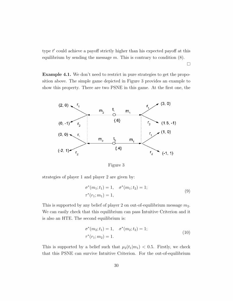
Example 4.1. We don’t need to restrict in pure strategies to get the propo-

sition above. The simple game depicted in Figure 3 provides an example to

show this property. There are two PSNE in this game. At the first one, the

Figure 3

strategies of player 1 and player 2 are given by:

σ∗(m1; t1) = 1, σ∗(m1; t2) = 1;

τ ∗(r1;m1) = 1,(9)

This is supported by any belief of player 2 on out-of-equilibrium message m2.

We can easily check that this equilibrium can pass Intuitive Criterion and it

is also an HTE. The second equilibrium is:

σ∗(m2; t1) = 1, σ∗(m2; t2) = 1;

τ ∗(r1;m2) = 1.(10)

This is supported by a belief such that µ2(t1|m1) < 0.5. Firstly, we check

that this PSNE can survive Intuitive Criterion. For the out-of-equilibrium

30

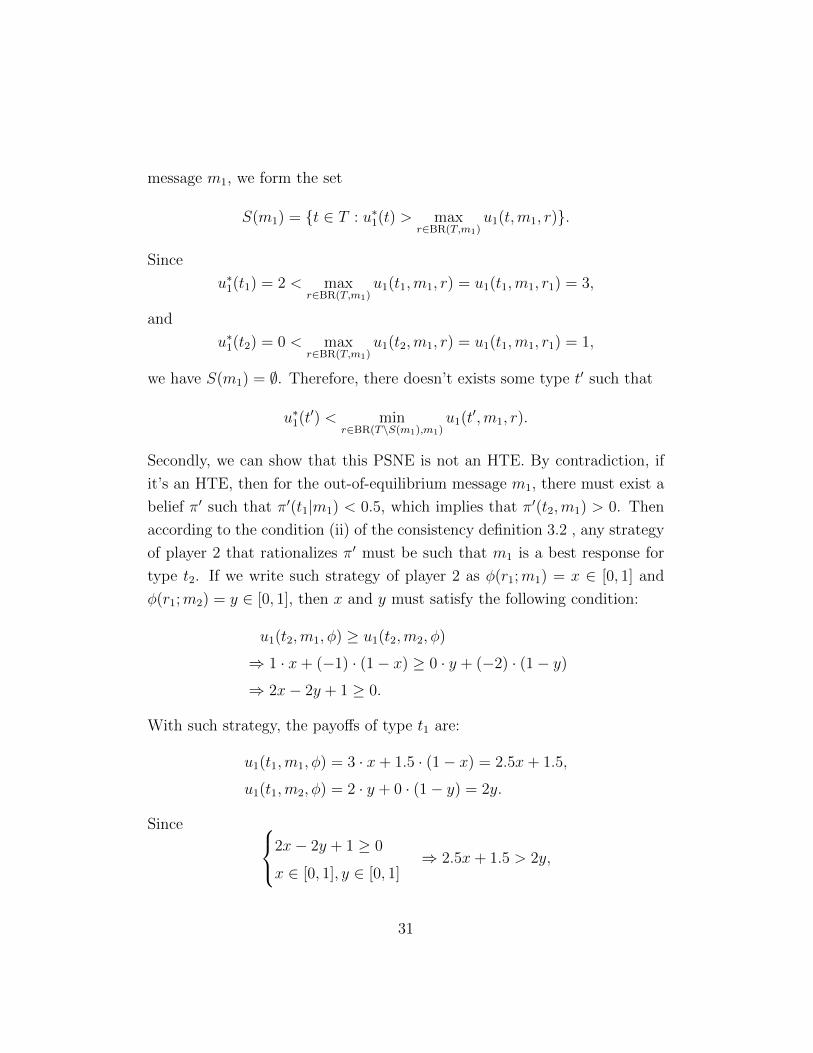
message m1, we form the set

S(m1) = t ∈ T : u∗1(t) > maxr∈BR(T,m1)

u1(t,m1, r).

Since

u∗1(t1) = 2 < maxr∈BR(T,m1)

u1(t1,m1, r) = u1(t1,m1, r1) = 3,

and

u∗1(t2) = 0 < maxr∈BR(T,m1)

u1(t2,m1, r) = u1(t1,m1, r1) = 1,

we have S(m1) = ∅. Therefore, there doesn’t exists some type t′ such that

u∗1(t′) < minr∈BR(T\S(m1),m1)

u1(t′,m1, r).

Secondly, we can show that this PSNE is not an HTE. By contradiction, if

it’s an HTE, then for the out-of-equilibrium message m1, there must exist a

belief π′ such that π′(t1|m1) < 0.5, which implies that π′(t2,m1) > 0. Then

according to the condition (ii) of the consistency definition 3.2 , any strategy

of player 2 that rationalizes π′ must be such that m1 is a best response for

type t2. If we write such strategy of player 2 as φ(r1;m1) = x ∈ [0, 1] and

φ(r1;m2) = y ∈ [0, 1], then x and y must satisfy the following condition:

u1(t2,m1, φ) ≥ u1(t2,m2, φ)

⇒ 1 · x+ (−1) · (1− x) ≥ 0 · y + (−2) · (1− y)

⇒ 2x− 2y + 1 ≥ 0.

With such strategy, the payoffs of type t1 are:

u1(t1,m1, φ) = 3 · x+ 1.5 · (1− x) = 2.5x+ 1.5,

u1(t1,m2, φ) = 2 · y + 0 · (1− y) = 2y.

Since 2x− 2y + 1 ≥ 0

x ∈ [0, 1], y ∈ [0, 1]⇒ 2.5x+ 1.5 > 2y,

31

which means that m1 is the unique best response for type t1. That is

π′(m1|t1) = 1. Therefore

π′(t1|m1) ≥ π′(m1|t1)π′(t1) = 0.6,

which is contrary to π′(t1|m1) < 0.5.

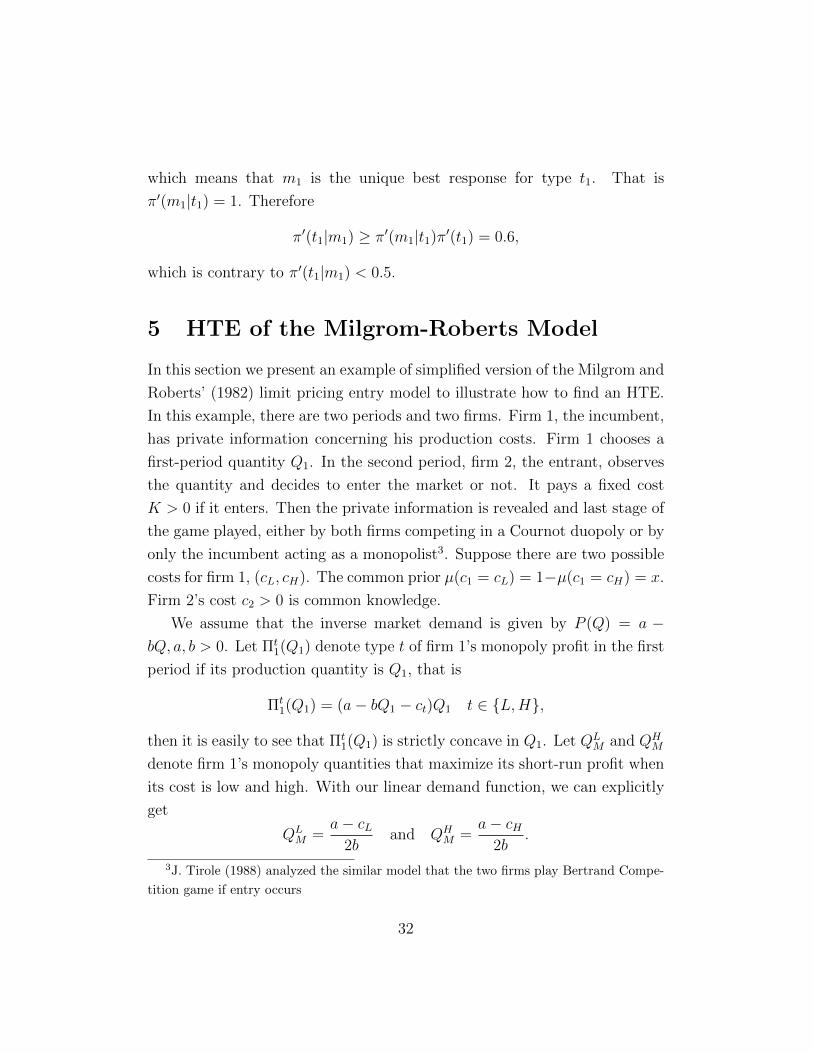
5 HTE of the Milgrom-Roberts Model

In this section we present an example of simplified version of the Milgrom and

Roberts’ (1982) limit pricing entry model to illustrate how to find an HTE.

In this example, there are two periods and two firms. Firm 1, the incumbent,

has private information concerning his production costs. Firm 1 chooses a

first-period quantity Q1. In the second period, firm 2, the entrant, observes

the quantity and decides to enter the market or not. It pays a fixed cost

K > 0 if it enters. Then the private information is revealed and last stage of

the game played, either by both firms competing in a Cournot duopoly or by

only the incumbent acting as a monopolist3. Suppose there are two possible

costs for firm 1, (cL, cH). The common prior µ(c1 = cL) = 1−µ(c1 = cH) = x.

Firm 2’s cost c2 > 0 is common knowledge.

We assume that the inverse market demand is given by P (Q) = a −bQ, a, b > 0. Let Πt

1(Q1) denote type t of firm 1’s monopoly profit in the first

period if its production quantity is Q1, that is

Πt1(Q1) = (a− bQ1 − ct)Q1 t ∈ L,H,

then it is easily to see that Πt1(Q1) is strictly concave in Q1. Let QL

M and QHM

denote firm 1’s monopoly quantities that maximize its short-run profit when

its cost is low and high. With our linear demand function, we can explicitly

get

QLM =

a− cL2b

and QHM =

a− cH2b

.

3J. Tirole (1988) analyzed the similar model that the two firms play Bertrand Compe-

tition game if entry occurs

32

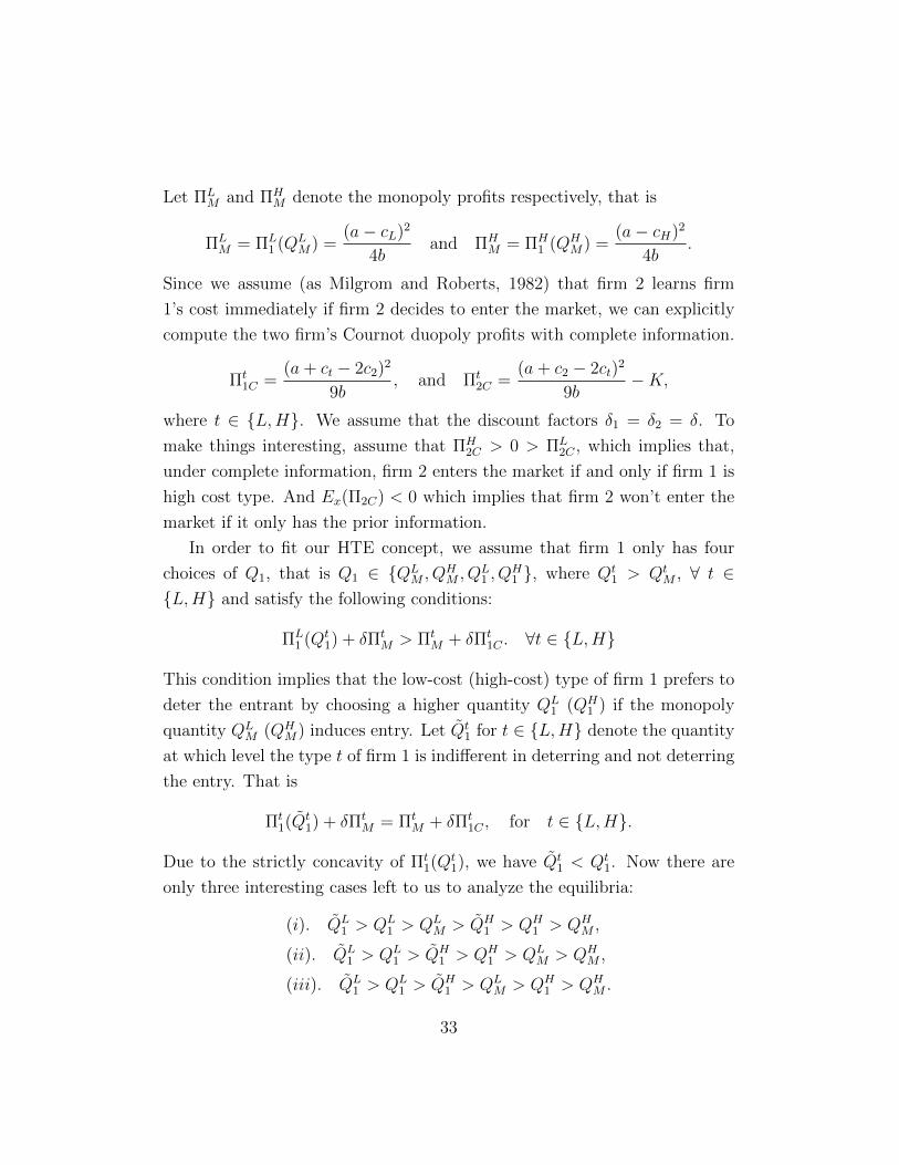
Let ΠLM and ΠH

M denote the monopoly profits respectively, that is

ΠLM = ΠL

1 (QLM) =

(a− cL)2

4band ΠH

M = ΠH1 (QH

M) =(a− cH)2

4b.

Since we assume (as Milgrom and Roberts, 1982) that firm 2 learns firm

1’s cost immediately if firm 2 decides to enter the market, we can explicitly

compute the two firm’s Cournot duopoly profits with complete information.

Πt1C =

(a+ ct − 2c2)2

9b, and Πt

2C =(a+ c2 − 2ct)

2

9b−K,

where t ∈ L,H. We assume that the discount factors δ1 = δ2 = δ. To

make things interesting, assume that ΠH2C > 0 > ΠL

2C , which implies that,

under complete information, firm 2 enters the market if and only if firm 1 is

high cost type. And Ex(Π2C) < 0 which implies that firm 2 won’t enter the

market if it only has the prior information.

In order to fit our HTE concept, we assume that firm 1 only has four

choices of Q1, that is Q1 ∈ QLM , Q

HM , Q

L1 , Q

H1 , where Qt

1 > QtM , ∀ t ∈

L,H and satisfy the following conditions:

ΠL1 (Qt

1) + δΠtM > Πt

M + δΠt1C . ∀t ∈ L,H

This condition implies that the low-cost (high-cost) type of firm 1 prefers to

deter the entrant by choosing a higher quantity QL1 (QH

1 ) if the monopoly

quantity QLM (QH

M) induces entry. Let Qt1 for t ∈ L,H denote the quantity

at which level the type t of firm 1 is indifferent in deterring and not deterring

the entry. That is

Πt1(Qt

1) + δΠtM = Πt

M + δΠt1C , for t ∈ L,H.

Due to the strictly concavity of Πt1(Qt

1), we have Qt1 < Qt

1. Now there are

only three interesting cases left to us to analyze the equilibria:

(i). QL1 > QL

1 > QLM > QH

1 > QH1 > QH

M ,

(ii). QL1 > QL

1 > QH1 > QH

1 > QLM > QH

M ,

(iii). QL1 > QL

1 > QH1 > QL

M > QH1 > QH

M .

33

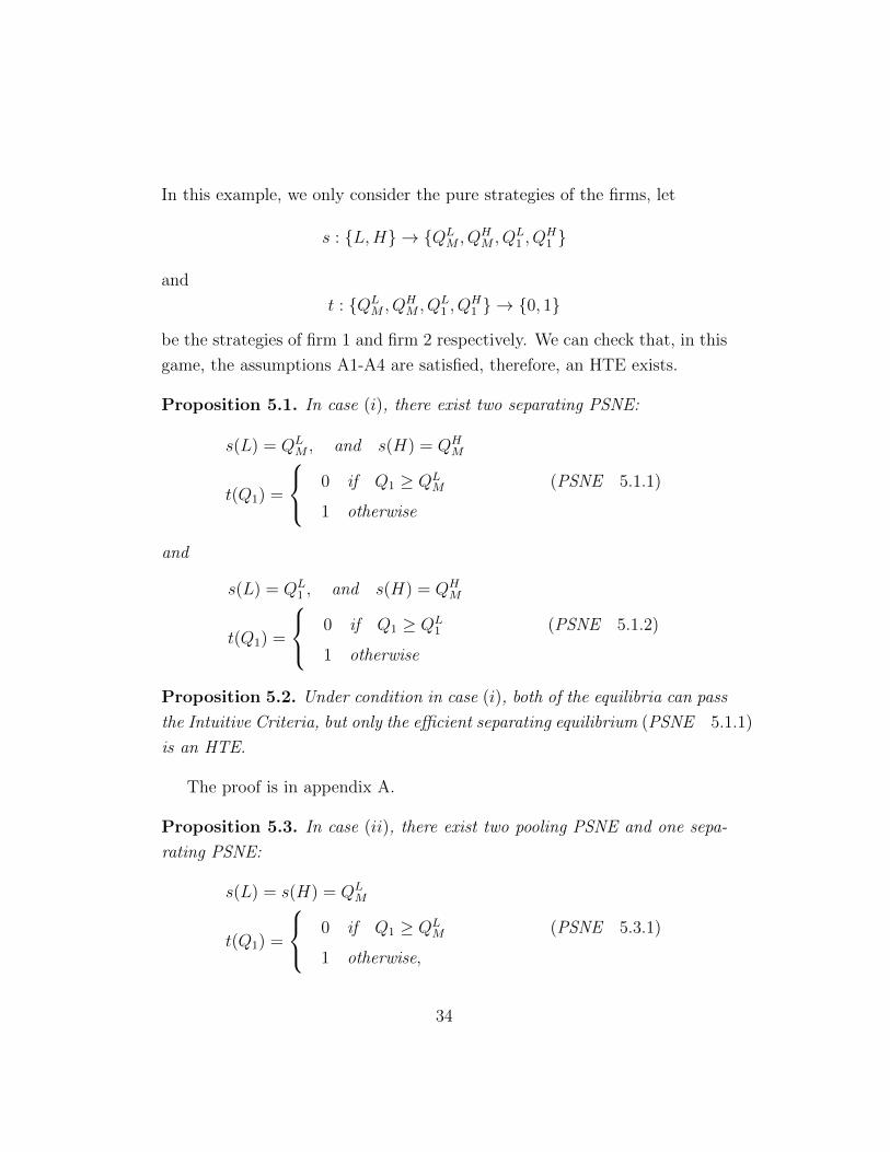
In this example, we only consider the pure strategies of the firms, let

s : L,H → QLM , Q

HM , Q

L1 , Q

H1

and

t : QLM , Q

HM , Q

L1 , Q

H1 → 0, 1

be the strategies of firm 1 and firm 2 respectively. We can check that, in this

game, the assumptions A1-A4 are satisfied, therefore, an HTE exists.

Proposition 5.1. In case (i), there exist two separating PSNE:

s(L) = QLM , and s(H) = QH

M

t(Q1) =

0 if Q1 ≥ QLM (PSNE 5.1.1)

1 otherwise

and

s(L) = QL1 , and s(H) = QH

M

t(Q1) =

0 if Q1 ≥ QL1 (PSNE 5.1.2)

1 otherwise

Proposition 5.2. Under condition in case (i), both of the equilibria can pass

the Intuitive Criteria, but only the efficient separating equilibrium (PSNE 5.1.1)

is an HTE.

The proof is in appendix A.

Proposition 5.3. In case (ii), there exist two pooling PSNE and one sepa-

rating PSNE:

s(L) = s(H) = QLM

t(Q1) =

0 if Q1 ≥ QLM (PSNE 5.3.1)

1 otherwise,

34

s(L) = s(H) = QH1

t(Q1) =

0 if Q1 ≥ QH1 (PSNE 5.3.2)

1 otherwise,

and

s(L) = QL1 , and s(H) = QH

M

t(Q1) =

0 if Q1 ≥ QL1 (PSNE 5.3.3)

1 otherwise

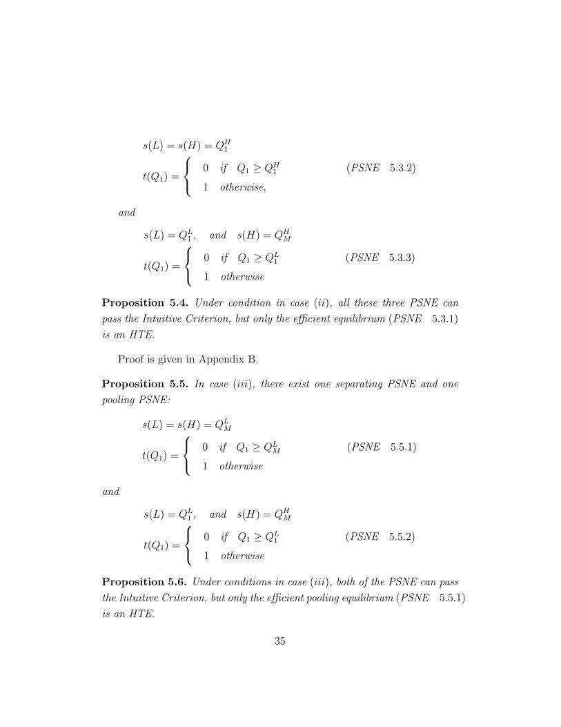
Proposition 5.4. Under condition in case (ii), all these three PSNE can

pass the Intuitive Criterion, but only the efficient equilibrium (PSNE 5.3.1)

is an HTE.

Proof is given in Appendix B.

Proposition 5.5. In case (iii), there exist one separating PSNE and one

pooling PSNE:

s(L) = s(H) = QLM

t(Q1) =

0 if Q1 ≥ QLM (PSNE 5.5.1)

1 otherwise

and

s(L) = QL1 , and s(H) = QH

M

t(Q1) =

0 if Q1 ≥ QL1 (PSNE 5.5.2)

1 otherwise

Proposition 5.6. Under conditions in case (iii), both of the PSNE can pass

the Intuitive Criterion, but only the efficient pooling equilibrium (PSNE 5.5.1)

is an HTE.

35

We can use almost the same argument as the proof of prop. 5.4 to prove

this proposition. So we omit the proof here.

To summarize this analysis of the limit pricing entry deterrence model: In

each case, there exists a unique HTE. At an HTE, the hight-cost type firm 1

either chooses its monopoly quantity and allows entry or makes pooling with

the low-cost type and deters the entry depending on the cost of pooling.

The low-cost type choose its monopoly quantity and entry doesn’t occur. By

contrast, in each case, there exist multi equilibria which can survive Intuitive

Criterion. At separating equilibrium (PSNE 5.1.2; PSNE 5.3.3; PSNE 5.5.2),

even though it is costly for the high-cost type to pool with the low-cost type,

the low-cost type firm 1 still needs to sacrifice its short-run profit and chooses

a higher quantity to distinguish himself from the high-cost type. We argue

that this type of equilibrium can’t be an HTE because there doesn’t exist a

rational belief system to support the equilibrium when an out-of-equilibrium

message QLM is observed.

6 Conclusions

In this paper, we propose a general definition of Hypothesis Testing Equilib-

rium (HTE) in a framework of general signaling games with Non-Bayesian

players. We focus on the analysis of a special class of HTE with threshold

ε = 0 as a method of equilibrium refinement which can survive the Intuitive

Criterion. For a broad class of signaling games, a Lexicographically Maxi-

mum sequential equilibrium is an HTE and the constrained HTE is unique.

In the example of limit pricing enter deterrence game, we show that there

exists unique HTE in each interesting case. However, there are aspects of

HTE we have not considered. In particular, the existence and uniqueness of

general HTE in more general signaling games, which we can’t get a concrete

conclusion. Natural extensions of HTE is to apply the concept in signal-

ing games in which the state space is infinite or for general dynamic games.

Without dynamic consistency, there will be some difficulties for these exten-

36

sions. Nevertheless, a further study of the general HTE in dynamic games is

encouraged.

37

APPENDIX

A. proof of proposition 5.2

Proof. To prove

s(L) = QLM , and s(H) = QH

M

t(Q1) =

0 if Q1 ≥ QLM

1 otherwise

is an HTE, we construct a Hypothesis Testing Model (ρ, 0) to support this

equilibrium. The support of ρ contains three elements: π0, π1, and π2 such

that ρ(π0 > ρ(π1) = ρ(π2) > 0. And they satisfy the following conditions:

(i). πi(L) = 1− πi(H) = x, ∀ i ∈ 0, 1, 2;(ii). π0(QL

M |L) = 1, π0(QHM |H) = 1;

(ii). π1(QL1 |L) = 1, π1(QH

M |H) = 1;

(ii). π2(QLM |L) = 1, π2(QH

1 |H) = 1.

We can check that π0 can be rationalized by the strategy

t(Q1) =

0 if Q1 ≥ QLM

1 otherwise;

π1 can be rationalized by the strategy

t(Q1) =

0 if Q1 ≥ QL1

1 otherwise;

and π2 can be rationalized by the strategy

t(Q1) =

0 if Q1 ≥ QH1

1 otherwise.

Firm 2 starts with π0 and keeps it for Bayesian updating if it observes QLM or

QHM .If firm 2 observes QL

1 , it switches to π1 and proceeds Bayesian Updating

38

because

π1(QL1 )ρ(π1) = π1(L)ρ(π1) > 0

π0(QL1 )ρ(π0) = π2(QL

1 )ρ(π2) = 0

Analogously, if firm 2 observes QH1 , it switches to π2. Clearly, given the

strategy s of firm 1, t is a best response of firm 2. Given t, under the

condition in case (i), we have:

u1(L,QLM , t(Q

LM) = 0) > u1(L,QL

1 , t(QL1 ) = 0),

u1(L,QLM , t(Q

LM) = 0) > u1(L,QH

1 , t(QH1 ) = 1),

u1(L,QLM , t(Q

LM) = 0) > u1(L,QH

M , t(QHM) = 1),

and

u1(H,QHM , t(Q

HM) = 1) > u1(H,QL

1 , t(QL1 ) = 0),

u1(H,QHM , t(Q

HM) = 1) > u1(H,QH

1 , t(QH1 ) = 1),

u1(L,QHM , t(Q

HM) = 1) > u1(H,QH

M , t(QHM) = 1),

Therefore, (s, t) is an HTE.

Now let’s prove that

s(L) = QL1 , and s(H) = QH

M

t(Q1) =

0 if Q1 ≥ QL1

1 otherwise

is not an HTE. We can check that when the out-of-equilibrium message QLM

is observed, for any µ2(·|QLM), such that

µ2(L|QLM)ΠL

2C + (1− µ2(L|QLM))ΠH

2C > 0,

there doesn’t exist a strategy of player 2 by which µ2(·|QLM) can be rational-

ized. Since ΠL2C < 0 < ΠH

2C , then µ2(H|QLM) = 1 − µ2(L|QL

M) must be big

enough, which implies µ2(QLM |H) > 0. By definition 3.1 (iii), any strategy

of firm 2 that rationalizes µ2 must be such that QLM is a best response for

39

type H. However, under condition in case (i), QLM > QH

1 , QLM would never

be a best response for type H because QLM is strictly dominated by QH

1 .

Now let’s check that both of the equilibria can pass the Intuitive Criterion.

In PSNE 5.3.1, S(QL1 ) = H, and S(QH

1 ) = L, however, there doesn’t

exist t′ such that condition (6) holds for QL1 and QH

1 .

B. proof of proposition 5.4

Proof. (PSNE 5.3.1) is an HTE supported Hypothesis Testing model (ρ, 0)

where the support of ρ contains four elements: π0, π1, π2 and π3 such that

ρ(πΩ) > ρ(π1) = ρ(π2) = ρ(π3) > 0. And they satisfy the following condi-

tions:

(i). π = 1− π = x, for all π ∈ supp(ρ);

(ii). π0(QLM |L) = 1, π0(QL

M |H) = 1;

(iii). π1(QLM |L) = 1, π1(QH

M |H) = 1;

(iv). π2(QH1 |L) = 1, π2(QH

1 |H) = 1;

(v). π3(QL1 |L) = 1, π2(QH

M |H) = 1.

(PSNE 5.3.2) is not an HTE. When QLM is observed, we show there

doesn’t exist a strategy of player 2 to rationalize any belief µ2 satisfying the

following conditions:

µ2(L) = 1− µ2(H) = x, and

µ2(L|QLM)ΠL

2C + µ2(H|QLM)ΠH

2C > 0.

By assumption:

ΠL2C < 0 < ΠH

2C and xΠL2C + (1− x)ΠH

2C < 0,

we can obtain that µ2(H|QLM) > x, therefore, µ2(H,QL

M) > 0, which implies

that any strategy of firm 2 rationalizes µ2 must be such that QLM is a best

response for type H. Since we restrict pure strategy, the strategy t : M → R

40

must satisfy t(QLM) = 0. But with this strategy, QL

M is the unique best

response for type L, that is µ2(QLM |L) = 1. Then

µ2(L|QLM) =

µ2(QLM |L)µ2(L)

µ2(QLM |L)µ2(L) + µ2(QL

M |H)µ2(H)

=x

x+ µ2(QLM |H)(1− x)

≥ x,

which is contradiction with µ2(L|QLM) < x.

We can use the similar argument to prove that PSNE (5.3.3) is not an

HTE. There doesn’t exist rational prior to support the out-of-equilibrium

message QLM . We also can show that this equilibrium can pass the Intuitive

Criterion because any out-of-equilibrium message m ∈ QLM , Q

H1 , we have

S(m) = ∅.

References

[1] Athey S., Single Crossing Properties and the Existence of Pure Strategy

Equilibria in Games of Incomplete Information, Econometrica, Vol. 69,

No. 4 (Jul., 2001), pp. 861-889.

[2] Banks J. S. and Sobel J. , Equilibrium selection in signaling Games,

Econometrica, Vol. 55, No. 3 (May, 1987), 647-661.

[3] Camerer, Colin , Individual decision making. In The Handbook of Exper-

imental Economics (John H. Kagel and Alvin E. Roth, eds.), Princeton

University Press, Princeton, 1995, 587703.

[4] Cho In-Koo, A Refinement of Sequential Equilibrium, Econometrica, Vol.

55, No. 6 (Nov., 1987), pp. 1367-1389.

[5] Cho In-Koo and Kreps David M., Signaling Games and Stable Equilibria,

The Quarterly Journal of Economics, Vol. 102, No. 2, (May, 1987), pp.

179-221.

41

[6] Epstein, Larry G. An axiomatic model of non-Bayesian updating. Review

of Eco- nomicStudies,73, 2006, 413436.

[7] Epstein, Larry G., Noor J., and Sandroni A., Non-Bayesian updating: a

theoretical framework, Theoretical Economics 3 (2008), 193229.

[8] Epstein, Larry G., Noor J., and Sandroni A., Non-Bayesian Learning,

The B.E. Journal of Theoretical Economics Advances, Volume 10, Issue

1, 2010,

[9] Foster D. P., and Young H. P. , Learning, hypothesis testing, and Nash

equilibrium, Games and Economic Behavior 45 (2003) 7396.

[10] Fudenberg D. and Tirole J.. Sequential bargaining with incomplete in-

formation. Review of Economic Studies, 50(2):221-247, April 1983.

[11] Fudenberg D. and Tirole J., Perfect Bayesian Equilibrium and Sequen-

tial Equilibrium, Journal of Economic Theory, 53, 236-260, 1991.

[12] Gilboa I, Postlewaite A, and Schmeidler D, Probability and uncertainty

in economic modelling, J. Econ. Perspectives 22 (2008), 173-188.

[13] Gilboa I, Postlewaite A, and Schmeidler D, Is it always rational to satisfy

Savages axioms?,Econ. and Phil. 25 (2009), 285-296.

[14] Gilboa I, Postlewaite A, and Schmeidler D, Rationality of belief or:

why Savages axioms are neither necessary nor sufficient for rationality,

Synethese, 2012

[15] Golub B., and Jackson M. O., Naıve Learning in Social Networks and

the Wisdom of Crowds, American Economic Journal: Microeconomics,

Vol. 2, No. 1 (February 2010), pp. 112-149.

[16] Govindan S. and Wilson R. , Global Newton Method for stochastic

games, Journal of Economic Theory Volume 144, Issue 1, Pages 414421,

January 2009.

42

[17] Govindan S., and Wilson R. , A decomposition algorithm for N-player

games, Econ. Theory (2008), in press, preprint: Res. Report 1967, Stan-

ford Business School.

[18] Govindan S. and Wilson R. , Axiomatic Equilibrium Selection for

Generic Two-Player Games, Econometrica, Volume 80, Issue 4, pages

16391699, July 2012.

[19] Hillas J. and Kohlberg E., Chapter 42 Foundations of strategic equilib-

rium, Handbook of Game Theory with Economic Applications, Volume

3, Pages 15971663, 2002.

[20] Kohlberg E. and Mertens J., On the Strategic Stability of Equilibria,

Econometrica, Vol. 54, No. 5 (Sep., 1986), pp. 1003-1037.

[21] Kreps D. M. and Wilson R. , Sequential Equilibria, Econometrica, Vol.

50, No. 4 (Jul., 1982), pp. 863-894.

[22] Leland Hayne E. and Pyle David H., Informational asymmetries, finan-

cial structure, and financial intermediation informational asymmetries,

financial structure, and financial intermediation. The Journal of Finance.,

32(2):371-387, May 1977.

[23] Mailath G, J, and Okuno-Fujiwara M. , Belief-based refinements in Sig-

naling games, Journal of Economic Theory, 60, 241-276, 1993.

[24] Man Priscilla T. Y. , Forward Induction Equilibrium games and eco-

nomic behavior, 2012.

[25] Milgrom P. and Roberts J., Limit Pricing and Entry under Incomplete

Information: An Equilibrium Analysis, Econometrica, Vol. 50, No. 2

(Mar., 1982), pp. 443-459.

[26] Mullainathan, Sendhil (2000), Thinking through categories. Unpub-

lished, Department of Economics, MIT.

43

[27] Ortoleva P. ,Modeling the Change of Paradigm: Non-Bayesian Reactions

to Unexpected News, American Economic Review, 102(6): 2410-36. 2012.

[28] Rabin, Matthew (2002), Inference by believers in the law of small num-

bers. Quarterly Journal of Economics,117,775816.

[29] Riley. John G., Silver signals: Twenty-five years of screening and signal-

ing. Journal of Economic Literature, 39(2):432-478, June 2001.

[30] Spence, A. Michael, Market Signaling (Cambridge, MA: Harvard Uni-

versity Press, 1974).

[31] Teng J. , A Bayesian Theory of Games: Iterative Conjectures and de-

termination of quilibrium, Chartridge Books Oxford, 2014 Rationality

of belief or: why savage’s axioms are neither necessary nor sufficient for

rationality

[32] Tversky, Amos and Daniel Kahneman (1974), Judgement under uncer-

tainty: Heuristics and biases. Science,185,11241131.

[33] Umbauer, G., Forward induction, consistency and rationality of ε per-

turbations, mimeo, Universite Louis Paster, Strasbourg, 1991.

[34] van Damme E., Chapter 41 Strategic equilibrium, Handbook of Game

Theory with Economic Applications Volume 3, Pages 15211596, 2002.

44