5306 IEEE TRANSACTIONS ON IMAGE PROCESSING, VOL. …download.xuebalib.com/xuebalib.com.48932.pdf ·...

5306 IEEE TRANSACTIONS ON IMAGE PROCESSING, VOL. 22, NO. 12, DECEMBER 2013

A Kalman Filter Approach for Denoising andDeblurring 3-D Microscopy Images

Francesco Conte, Alfredo Germani, and Giulio Iannello, Member, IEEE

Abstract— This paper proposes a new method for removingnoise and blurring from 3D microscopy images. The maincontribution is the definition of a space-variant generating modelof a 3-D signal, which is capable to stochastically describe awide class of 3-D images. Unlike other approaches, the space-variant structure allows the model to consider the informationon edge locations, if available. A suitable description of theimage acquisition process, including blurring and noise, is thenassociated to the model. A state-space realization is finallyderived, which is amenable to the application of standard Kalmanfilter as an image restoration algorithm. The so obtained methodis able to remove, at each spatial step, both blur and noise,via a linear minimum variance recursive one-shot procedure,which does not require the simultaneous processing of the wholeimage. Numerical results on synthetic and real microscopy imagesconfirm the merit of the approach.

Index Terms— Kalman filters, image restoration, deconvolu-tion, state-space methods, optical microscopy.

I. INTRODUCTION

IN RECENT times, the exploration of the microscopic3-D structures of living biological cells and tissues has

been made possible [1] by the availability of sophisticated3-D optical instruments [2]. Several microscopy techniqueshave been developed, such as Widefield Microscopy, ConfocalMicroscopy [3], Light-Sheet Microscopy (LSM) [4]–[7]. Inorder to take full advantage of these instruments, severalcomputational methods for restoring and enhancement of3-D images have been proposed (e.g. [8]–[10]). In particular,a great deal of attention has been dedicated to the develop-ment of algorithms capable to remove the noise disturbances,usually introduced by digital detectors (e.g. CCD cameras),and correct the so called blurring effect. The latter is caused

Manuscript received June 21, 2012; revised November 1, 2012 andFebruary 11, 2013; accepted August 30, 2013. Date of publication October9, 2013; date of current version October 28, 2013. This work was supportedin part by the International Center of Computational Neurophotonics and inpart by the Consorzio interuniversitario per le Applicazioni di SupercalcoloPer Universitá e Ricerca which provided computational and storage resourcesunder Projects std11-449 and std12-131. The associate editor coordinat-ing the review of this manuscript and approving it for publication wasProf. Brian D. Rigling.

F. Conte and A. Germani are with the Dipartimento di Ingegneria e Scienzedell’Informazione e Matematica, Università degli studi dell’Aquila, L’Aquila67100, Italy (e-mail: [email protected]; [email protected]).

G. Iannello is with the Università Campus Bio-Medico di Roma, Rome00128, Italy (e-mail: [email protected]).

This paper has supplementary downloadable material available athttp://ieeexplore.ieee.org., provided by the author. The multimedia packagecontains the “3-D Kalman Deconvolution Toolbox”, which is a Matlab GuiVersion of the algorithms Space-Independent Kalman Deconvolution (SIKD)and Space-Dependent Kalman Deconvolution (SDKD) for denoising anddeblurring 3-D images. There is also a toy demo. The total size of the file is188 KB. Contact [email protected] for further questions about this work.

Color versions of one or more of the figures in this paper are availableonline at http://ieeexplore.ieee.org.

Digital Object Identifier 10.1109/TIP.2013.2284873

by the physical low-pass behaviour of optical systems, whichdetermines loss of sharp variation points, with an immediateleak of resolution. From the modern biological point of view,this is a strong limitation since blurred images do not offerthe possibility to resolve sub-cellular phenomena [10].

As well as in the 3-D case, blurring occurs in several 2-Dimages (e.g. photographs, telescopes [11], microscopes, satel-lite sensors [12], etc.). As a consequence, the deblurring prob-lem (also called deconvolution) has been widely investigatedin the simpler 2-D case and then extended to the 3-D one.Classical approaches are Wiener filtering [13] and regularizedlinear least square (LLS) algorithms [14], [15]. These methodsmay suffer from noise amplification and artifacts generation.As a consequence, a regularization term is introduced, whichreduces the contributions of high spatial frequencies to theimage, where the noise component is dominant. Obviously,this also reduces the image sharpness. Moreover, regularizedLLS methods may estimate negative intensities in the restoredimage that generate artifacts. In order to solve this problem,nonlinear iterative constrained methods like the Tikhonov-Miller algorithm (ICTM) [16] and the Carrington algorithm[17] minimize the sum of the squared error between theacquired image and the estimated one by incorporating a non-negativity constraint. This additive information is enough toobtain a good image quality, making these methods widelyused. Nevertheless, the deconvolution results and the con-vergence rate strongly depend on the regularization parame-ter [18]. Thus, additional algorithms need to be executedin order to choose the optimal value for the regularizationparameter, which still determines the image sharpness level.

Unlike the above mentioned solutions, the maximum like-lihood (ML) approaches [1], [19], [20] explicitly take intoaccount the random nature of noise. Such methods are capableof restoring high noise images, especially for the particularcase of Poisson noise. Nevertheless, there are a few drawbacks.First of all, the performance improvement is paid with asignificant increase of computational burden. Moreover, thebasic algorithm converges to noise asymptotically and thusrequires regularization, with a further computational load.

The regularization of ML methods can be obtained byusing expectation maximization (EM) or the maximum aposteriori (MAP) approach. The EM uses penalized maxi-mum likelihood (PML) criteria. Examples can be found in[21]–[23], and [1]. The MAP idea is to get regularizationby supposing the original image to be distributed with agiven probability density (prior, from a Bayesian point ofview). By this approach, several algorithms have been devel-oped adopting different regularizers such total-variation (TV)[24]–[27], wavelet-based [28], or �1 norm [29]. Further recent

1057-7149 © 2013 IEEE

CONTE et al.: A KALMAN FILTER APPROACH FOR DENOISING AND DEBLURRING 3-D MICROSCOPY IMAGES 5307

works such as [30]–[32] are devoted to the improvement ofMAP algorithms in terms of computational efficiency.

There also exist MAP methods based on a realistic priorknowledge of the original image. In e.g. [33] the key ideaconsists in considering the latter as a realization of a randomfield with a given probability distribution. The solutions pro-vided by these methods are stable and very accurate thanksto the use of a priori information about the original image,which is generally paid with a significant computational load.In many practical situations, it is unrealistic to assume thata consistent estimation of the image gray-level distribution isavailable and therefore, preliminary high dimensional parame-ter identification procedures are always required.

All the above mentioned methods assume to have at onedisposal the complete knowledge of the blurring kernel, usu-ally named Point Spread Function (PSF). When this is notthe case, methods capable to identify the PSF and restore theimage in the same time have been developed. Such algorithmsare commonly referred to as blind deconvolution methods (e.g[34]–[38]).

In this paper, we extend the main idea of [39]–[42], and[43] for 2-D images, to propose a new (non blind) filteringand deblurring method. The approach is based on physical-likeassumptions about the structure of the 3-D stochastic imagemodel, without using any a priori knowledge of the imagegray-level distribution. In a natural way, the assumptions madeallow defining a 3-D consistent model for the “generatingprocess” of the original 3-D image, which is amenable to theimplementation of a Kalman-based minimum variance linearestimation algorithm. Moreover, in order to take into accountextra information concerning the position of edge voxels, aspace-dependent filtering algorithm is proposed having thespecial feature of significantly reducing blurring effects. Ofcourse, in this case, stationary Kalman filtering is not moreusable and, therefore, computational complexity turns out tobe strongly augmented. A first attempt of designing a 3-Ddeblurring procedure by the definition of an image recursivestate model is given in [44].

We remark here that our contributions with respect to thisapproach consist in: a) extension of the model to the 3-D case,b) embedding of the deblurring task into the algorithm, andc) the possibility to use the information on edge locationswhich is a novelty in the deblurring methods literature.

To a large extent, the so obtained method satisfies thefollowing list of desirable features for a filtering and deblurringprocedure: i) dependency on a few and easily identifiableparameters; ii) avoidance of artifacts generation; iii) simul-taneous filtering and deblurring procedure; iv) optimality withrespect to the assumed generating model; v) recursive struc-ture, in order to require at each step a lower memory amount;vi) computationally one-shot, in order to avoid the difficultchoice of a suitable stopping criterion; vii) extensible tothe edge-dependent form; viii) readily implementable; ix)endowed with stability and robustness; x) amenable to beefficiently parallelized.

The paper is organized as follows. Section II formalizesthe three dimensional deconvolution problem. In Sections IIIand IV the image model is defined. The restoration algorithm

is described in Section V. Results are reported in Section VI.Finally, conclusions are summarized in Section VII.

II. PROBLEM FORMULATION

Without loss of generality, we here only consider a 3-Dmonochromatic image. This can be described by a spatialsignal x : � ⊂ R

3 → [0 1], where � is assumed to be a closedrectangular box in R

3 and x(p) indicates the gray-level of theoriginal image at the spatial coordinate p = [r s t]T ∈ �. Thecorresponding sampled image is denoted by

xi, j,k := x(i�r , j�s, k�t ), (1)

with i, j = 1, . . . , l, and k = 1, . . . , H , and where �r , �s ,and �t are the spatial sampling intervals on the three maindirections. As usual, the image volume about the discretespatial coordinate (i, j, k) will be hereafter referred to as voxel.Moreover, we will indicate by i = a : b the finite integers’sequence i = a, a + 1, . . . , b.

We suppose the 3-D image composed by a series (stack)of H 2-D l × l images, called slices. Each of them is hereidentified by the third index k. Whereas, pair (i, j) indicatesthe 2-D discrete coordinate within the considered slice.

The term original image is referred to the ideal represen-tation of the recorded object. The goal of this paper is todesign a restoration algorithm able to provide an estimationof this signal from an image acquisition affected by blurringand noise, hereafter referred to as acquired image. The gray-level of this image measurement at voxel (i, j, k) is denotedby yi, j,k . In this paper, a noise additive model is considered:

yi, j,k = (h ∗ x)i, j,k + vi, j,k , (2)

where (h ∗ x)i, j,k denotes the sampled convolution betweenthe Point Spread Function (PSF) h : � ⊂ R

3 → [0 1] andthe original image for modelling the blurring, and vi, j,k is thenoise corrupting voxel (i, j, k).

The convolution term can be expressed in the followingform:

(h ∗ x)i, j,k =br∑

l=−ar

bs∑

m=−as

bt∑

n=−at

hl,m,n · xi−l, j−m,k−n , (3)

where hl,m,n denotes the sampled PSF. Note that latter is heresupposed to be space-limited. More precisely, integer intervals[−ar , br ], [−as, bs], and [−at , bt ], containing zero, are thediscrete supports of the PSF along the three spatial directions.For the sequel, it will be useful to recognize the extent ofthe PSF on the three directions as ωd := ad + bd + 1, withd = r, s, t . Without loss of generality, the volume of h issupposed to be equal to 1. In addition, the PSF is assumedto be completely known. In many cases this is an actualcondition. Indeed, literature provides several experimental set-ups (e.g. [10], [45], [46]) to the PSF estimation, which can beconsidered as only depending on the features of the opticalinstrument.

As far as the noise disturbance is concerned, it is assumedthat the noise corrupting a given voxel is zero-mean and notcorrelated with that corrupting a different voxel, i.e.

E[vi, j,kvl,m,n

] = δi,lδ j,mδk,nσ 2v , (4)


where, hereafter, δr,s indicates the Kronecker delta and σ 2v is

the noise variance. It is worth noting that no hypothesis ismade on the noise distribution. The usual acquisition modelfor microscopy images uses the Poisson distribution, moreprecisely:

yi, j,k = 1

cmP(cm (h ∗ x)i, j,k

), (5)

where P(c) denotes a process with Poisson statistics and ratec, and cm is the maximum photons counting number. Model(5) can be easily expressed in the in the additive form (2):

yi, j,k = (h ∗ x)i, j,k + 1

cmP(cm (h ∗ x)i, j,k

) − (h ∗ x)i, j,k

︸︷︷︸=:vi, j,k

.

(6)Appendix A shows that the so defined vi, j,k is zero-mean andthat a consistent estimate of the variance σ 2

v can be derived. Itis worth stressing that although the use of such an estimatedvariance constitutes an approximation for the Poisson model,the experimental results suggest that this simplification doesnot introduce significant disadvantages.

The filtering and deblurring problem requires the estimationof the discrete signal xi, j,k from the measurement yi, j,k , takinginto account the acquisition function (4).

III. THE IMAGE MODEL

A. The Image Signal: Basic Assumptions

In this section, a mathematical model for the generatingprocess of the original image is defined following an approachsimilar to the one given in [39], [40] for the 2-D case. Asfirst step, we state three physical-like hypothesis on the imagesignal x : � → [0 1]:

1) Smoothness assumption: the image domain � is con-stituted by the union of disjointed subregions �s ⊆ �such that

⋃s �s = � and any restriction x |�s is of class

Cν(�s).2) Stochastic assumption: all the derivatives of order ν +1

of the 3-D signal x are modelled by means of zero-meanindependent Gaussian random fields.

3) Inhomogeneity assumption: the random fields represent-ing the image process relative to different subregions areindependent.

Assumptions 1) and 2) are based on the consideration thatmost images are composed of open disjoint subregions whoseinterior is regular enough to be well described as a finitesupport restriction of a smooth three-dimensional Gaussianprocess. The degree of smoothness depends on the partic-ular considered image. The boundary of each subregion isconstituted by the image edges, which correspond to sharpdiscontinuities in the distribution of the gray-level. Assumption3) means that no correlation can be assumed among voxelsbelonging to different subregions. In this way, the edges canbe directly taken into account by the image model. The use ofsuch an information may allow improving the quality of therestored image by avoiding the introduction of spatial artifacts.

The edge locations can be obtained by a suitable edge-detector (e.g. [47]–[50]). Obviously, blurring could makethese algorithms able to only return approximate locations,

or sometimes to be completely unable to get consistent results.As a consequence, the edge locations have to be intended asan additive information that may be available or not.

As described below in the paper, assumptions 1), 2) and 3)generally allow defining a space-variant model that describesan image generating process taking into account the edgelocations, supposed to be available. In this case, the optimalrestoration procedure is guaranteed by the corresponding non-stationary Kalman filter. When the edge locations are notavailable, the model is reduced to a space-invariant form. If,from the one hand, this may reduce the model accuracy, onthe other hand, the use of stationary Kalman filter [51] asoptimal image restoration algorithm is made possible, with asignificant advantage in terms of computational load.

In the following, we will first derive the general space-variant image model. The invariant version will be then easilyobtained as a particular case.

B. The Homogeneous Image Equation

According to Assumption 1), a complete description of a3-D image can be given by means of the gray-level signal x(p)together with its partial derivatives, up to a certain order ν.As a consequence, considering the image signal x(p) inside asmooth region, it is possible to define a state vector composedof such a signal and its partial derivatives with respect to thespatial coordinates r , s, and t:1

X (p) :=[

∂�x(p)

∂r�−α∂sα−λ∂ tλ,� = 0 : ν; α = 0 : �; λ = 0 : α

]T

.

(7)The dimension of X (p) is n := (ν + 3)(ν + 2)(ν + 1)/3!.Details on the structure of X (p) are given in Appendix B-A.We are interested in studying the relation between the valueof the state vector at two different spatial positions. Therefore,let

p(u) = p + vu, v = [γ, β, δ]T

denote a parametric representation in u of a straight linepassing through the point p = [

r , s, t]T . As a direct

consequence of the state vector definition (7), the followingequation can be written:

X(p(u)) = γ

(∂

∂rX (p (u))

)

+ β

(∂

∂sX (p (u))

)+ δ

(∂

∂ tX (p (u))

), (8)

the dot denoting the derivative with respect to u. Moreover,by direct computation, we have:

∂∂d X (p (u)) = Ad X (p(u)) + BWd(p(u)), (9)

with d = r, s, t , respectively, and where: Ar , As , and At

are n × n commuting matrices, suitably defined to selectthe elements of the partial derivatives in (9) that belong tothe state vector X (p(u)). The general expressions for thesematrices are provided in Appendix B-B. As an example, we

1In (7) and hereafter, when multi-indices are used we assume that the rightindex increases before the left one (e.g. in (7) λ increases for a given couple(α, �) and α increases for a given �).


here report the simplest cases of order 0 and 1: Ar = As =At = 0, for ν = 0, and

Ar =[

0 1 0 003×4

], As =

[0 0 1 0

03×4

],

At =[

0 0 0 103×4

],

for ν = 1, where, hereafter, 0n×m denotes the n × m nullmatrix; B is the following n × m matrix, with m := (ν + 2)(ν + 1)/2:

B =[

0(n−m)×m

Im

],

where, hereafter, Im denotes the identity matrix in Rm ; vectors

Wr (p(u)), Ws(p(u)), and Wt (p(u)) have dimension m and aregiven by

Wd (p(u))=[

∂ν+1x(p)

∂rν−α∂sα−λ∂ tλ∂d,α = 0 : ν;λ = 0 : α

]T

,

(10)with d = r, s, t , respectively. Using (9), (8) can be rewrittenas

X(p(u)) = (γ Ar + β As + δAt ) X (p(u))

+B[γ Wr (p(u))+βWs(p(u))+δWt(p(u))

]. (11)

Formal integration of (11) with respect to u between u0 andu1 allows us to derive a relation between the state vectorsevaluated at two generic points p0 = [r + γ u0, s + βu0, t +δu0]T and p1 = [r + γ u1, s + βu1, t + δu1]T . Exploiting thecommutativity of Ar , As , and At , we obtain:

X (p1) = e(γ Ar +β As +δAt )(u1−u0) X (p0)

+∫ u1

u0

e(γ Ar +β As +δAt )(u1−τ ) B

· [γ Wr (p(τ )) + βWs(p(τ )) + δWt (p(τ ))]

dτ.

(12)

By the stochastic assumption, Wr (·), Ws(·), and Wt (·) arewhite Gaussian vector fields, so the integral term in (12) isintended as a stochastic Wiener integral.

C. The Component Equations of the Sampled Image

Results of Section III-B are here used in order to get asemicausal statistical model for the sampled image. Recallingthat xi, j,k denotes the value of the sampled original imageat point (i�r , j�s, k�t ), i, j = 1 : l, and k = 1 : H , therelevant sampled state vector is denoted by

Xi, j,k := X (i�r , j�s, k�t ). (13)

We assume that the image state vector at voxel (i, j, k)depends on the state vector at neighbouring voxels accordingto the scheme shown in Fig. 1, where, in order to simplifythe reconstruction algorithm, causality is only assumed for thethird coordinate (semicausal model).

Coefficients c(μ)i, j,k(μ = 1 : 5) may be 0 or 1. According

to the inhomogeneity assumption, they are equal to one if thecorresponding voxels belong to the same subregion, and equalto zero otherwise. This implies that 25 different configurations

Fig. 1. Spatial structure of semicausal dependence model.

of the image model can be obtained depending on the edgeshape at voxel (i, j, k).

The relations between the state vector Xi, j,k at voxel (i, j, k)and the state evaluated at neighbouring voxels for whichc(μ)

i, j,k = 1 can be obtained by applying (12), with a suitablechoice of γ , β, and δ. This allows deriving the followingcomponent equations:

c(1)i, j,k Xi, j,k = c(1)

i, j,k

(eAt �t Xi, j,k−1 + W (1)

i, j,k

), (14a)

c(2)i, j,k Xi, j,k = c(2)

i, j,k

(eAs�s Xi, j−1,k + W (2)

i, j,k

), (14b)

c(3)i, j,k Xi, j,k = c(3)

i, j,k

(eAr �r Xi−1, j,k + W (3)

i, j,k

), (14c)

c(4)i, j,k Xi, j,k = c(4)

i, j,k

(e−As �s Xi, j+1,k + W (4)

i, j,k

), (14d)

c(5)i, j,k Xi, j,k = c(5)

i, j,k

(e−Ar �r Xi+1, j,k + W (5)

i, j,k

), (14e)

where

W (1)i, j,k =

∫ 1

0�t e

At �t τ BWt (i�r , j�s, (k − τ )�t ) dτ, (15a)

W (2)i, j,k =

∫ 1

0�seAs �sτ BWs (i�r , ( j − τ )�s , k�t ) dτ, (15b)

W (3)i, j,k =

∫ 1

0�r eAr �r τ BWr ((i − τ )�r , j�s, k�t ) dτ, (15c)

W (4)i, j,k = −

∫ 1

0�se−As�sτBWs (i�r , (j +τ )�s, k�t )dτ, (15d)

W (5)i, j,k = −

∫ 1

0�r e−Ar �r τBWr ((i +τ )�r , j�s, k�t ) dτ. (15e)

Note that only the component equations for which c(μ)i, j,k are

equal to one give significant information. If some c(μ)i, j,k is null,

a trivial relation is obtained because (12) cannot be integratedalong that direction.

In order to simplify the mathematical development, we willindicate the voxels coordinates with the following notation:

(i, j, k)1 := (i, j, k), (i, j, k)2 := (i, j − 1, k),

(i, j, k)3 := (i − 1, j, k), (i, j, k)4 := (i, j + 1, k),

(i, j, k)5 := (i + 1, j, k);moreover, we define:

H1 := eAt �t , H2 := eAs�s , H3 := eAr �r , (16)

H4 := e−As �s , H5 := e−Ar �r . (17)


Finally, let pi, j,k denote the number of non-zero coefficientsc(μ)

i, j,k(μ = 1 : 5), voxel (i, j, k) is said to be internal, boundaryor isolated if pi, j,k = 5, 1 ≤ pi, j,k ≤ 4, pi, j,k = 0,respectively.

D. Modelling the State Noise

From the stochastic assumption and using (15a)–(15e), it ispossible to show that W (μ)

i, j,k(μ = 1 : 5) are zero-mean discreteGaussian random fields with the following properties:

E[W (1)

i, j,k W (1)T

l,m,n

]= δi,lδ j,mδk,n Qt , (18)

E[W (2)

i, j,k W (2)T

l,m,n

]= δi,lδ j,mδk,n Qs , (19)

E[W (3)

i, j,k W (3)T

l,m,n

]= δi,lδ j,mδk,n Qr , (20)

E[W (μ)

i, j,k W (μ)T

l,m,n

]= 0, ∀μ, μ ∈ {1, 2, 3} : μ = μ, (21)

with

Qd = �d

∫ 1

0eAd�dτ B�d BT eAT

d �dτ dτ, (22)

for d = r, s, t . Matrices �r , �s , and �t are such that,E[Wd (p) W T

d (p)] = �dδ (‖p − p‖), for any p, p ∈ R3 and

d = r, s, t ,. Estimates of �r , �s , and �t can be obtained asfunctions of the image spectrum, as showed in [39] for the2-D case. From (15a)–(15e), the following identities can beproved to hold:

W (4)i, j,k = −H4W (2)

i, j+1,k , (23)

W (5)i, j,k = −H5W (3)

i+1, j,k . (24)

The previous identities, obtained by assuming c(μ)i, j,k = 1, (μ =

2 : 5), imply the following relations among the covariancematrices of the Gaussian random fields W (μ)

i, j,k , (μ = 2 : 5):

E[W (4)

i, j,k W (4)Tl,m,n

]= δi,lδ j,mδk,n H4 Qs H T

4 , (25)

E[W (5)

i, j,k W (5)Tl,m,n

]= δi,lδ j,mδk,n H5Qr H T

5 . (26)

The statistics of the infinite three-dimensional Gaussianprocess corresponding to a generic smooth subregion is com-pletely defined by (18)–(21) and (25)–(26). As a consequence,these equations define the statistics for any voxel of eachsubregion. Of course, some of right-hand sides of (23) and (24)might lose their physical meaning in the presence of an edge,but the statistical meaning is retained, since it is related to theinfinite three-dimensional random field. Therefore, relations(25)–(26) are considered true even if some c(μ)

i, j,k = 0.

E. The Constitutive Equation

Assuming pi, j,k > 0, we now exploit the componentequations in order to derive a unique relation among Xi, j,k

and the state evaluated at its pi, j,k neighbouring voxels. Thisequation will be called constitutive equation (CE) as in [40],[41], and [43]. The case pi, j,k = 0 (isolated voxels) will beconsidered separately.

For convenience, we define c(μ)i, j,k := 1 − c(μ)

i, j,k , for μ =1 : 5; moreover, note that, considering the image dimensionsl × l × H , for any i, j = 1 : l, and k = 1 : H , it results that

c(1)i, j,1 = c(2)

i,1,k = c(3)1, j,k = c(4)

i,l,k = c(5)l, j,k = 0; (27)

c(4)i, j,k = c(2)

i, j+1,k, c(5)i, j,k = c(3)

i+1, j,k . (28)

Let us now consider one of (14b)–(14e). It relates thestate vector at voxel (i, j, k) with the state vector at a givenneighbouring voxel (i, j, k)μ (μ = 2 : 5). Vector X(i, j,k)μ canbe substituted with the right-hand of (14a). Such a substitutioncan be carried out only when the considered version of (14a)has significance, namely when the corresponding coefficientc(1)(i, j,k)μ

is equal to one. In order to keep the significance of the

new equation, c(1)(i, j,k)μ

is included in the substitution. On the

other hand, when c(1)(i, j,k)μ

is null, the correlation among the twovoxels involved in the equation needs to be kept. Therefore, itseems natural to consider such a voxel as an initial condition,namely, to assume

X(i, j,k)μ= X0

(i, j,k)μ+ W 0

(i, j,k)μ, (29)

where X0(i, j,k)μ

∈ Rn is externally imposed and W 0

(i, j,k)μis a

zero-mean white discrete Gaussian random field satisfying

E[W 0

i, j,k W 0T

l,m,n

]= δi,lδ j,mδk,n Qx0 . (30)

The covariance matrix Qx0 ∈ Rn×n is the (inverse) measure

of reliability of the external data.By following the described procedure, we derive, for any

μ = 2 : 5,

c(1)i, j,k Xi, j,k = c(1)

i, j,k H1X(i, j,k−1)1 + c(1)i, j,k W (1)

i, j,k , (31)

c(μ)i, j,k Xi, j,k = c(μ)

i, j,k

(c(1)(i, j,k)μ

HμH1X(i, j,k−1)μ

+ c(1)(i, j,k)μ

HμX0(i, j,k)1

)+ c(μ)

i, j,k

(c(1)(i, j,k)μ

HμW (1)(i, j,k)μ

+ c(1)(i, j,k)μ

HμW 0(i, j,k)μ

+ W (μ)i, j,k

), (32)

which can be rewritten in the compact form:

c(μ)i, j,k Xi, j,k = c(μ)

i, j,k Z (μ)i, j,k + c(μ)

i, j,k N (μ)i, j,k , μ = 1 : 5, (33)

where, for μ = 2 : 5:

Z (1)i, j,k := H1X(i, j,k−1)1 (34)

Z (μ)i, j,k := c(1)

(i, j,k)μHμH1 X(i, j,k−1)μ + c(1)

(i, j,k)μHμX0

(i, j,k)μ,

N (1)i, j,k := W (1)

i, j,k ,

N (μ)i, j,k := c(1)

(i, j,k)μHμW (1)

(i, j,k)μ+ c(1)

(i, j,k)μHμW 0

(i, j,k)μ+ W (μ)

i, j,k .

We want to combine such equations in order to obtain aunique relation with a minimum variance stochastic term. Itcan be proved that such a term can be expressed as weightedmean of the multivariate variables at the right-hand sides of(31)–(32), as follows:

Xi, j,k =⎛

⎝5∑

μ=1

�(μ)i, j,k

⎞

⎠−1

5∑

μ=1

�(μ)i, j,k

(Z (μ)

i, j,k + N (μ)i, j,k

), (35)


where the weight matrices �(μ)i, j,k are defined as

�(μ)i, j,k := c(μ)

i, j,k E[

N (μ)i, j,k N (μ)T

i, j,k

]−1. (36)

Taking into account the definition of N (μ)i, j,k , the statistical

properties of the state noise given by (18)–(21), (23)–(26) and(28), it can be shown that matrices �

(μ)i, j,k are well defined and

can be expressed in the form

�(μ)i, j,k = �

(μ)i, j,k + �

(μ)i, j,k, μ = 1 : 5, (37)

with:

�(1)i, j,k = c(1)

i, j,k Q−1t , (38)

�(2)i, j,k = c(2)

i, j,kc(1)(i, j,k)2

(H2 Qt H T

2 + Qs

)−1, (39)

�(3)i, j,k = c(3)

i, j,kc(1)(i, j,k)3

(H3Qt H T

3 + Qr

)−1, (40)

�(4)i, j,k = c(4)

i, j,kc(1)(i, j,k)4

(H4 (Qt + Qs) H T

4

)−1, (41)

�(5)i, j,k = c(5)

i, j,kc(1)(i, j,k)5

(H5 (Qt + Qr ) H T

5

)−1, (42)

�(1)i, j,k = 0n×n, (43)

�(2)i, j,k = c(2)

i, j,k c(1)(i, j,k)2

(H2 Qx0 H T

2 + Qs

)−1, (44)

�(3)i, j,k = c(3)

i, j,k c(1)(i, j,k)3

(H3Qx0 H T

3 + Qr

)−1, (45)

�(4)i, j,k = c(4)

i, j,k c(1)(i, j,k)4

(H4

(Qx0 + Qs

)H T

4

)−1, (46)

�(5)i, j,k = c(5)

i, j,k c(1)(i, j,k)5

(H5

(Qx0 + Qr

)H T

5

)−1. (47)

We remark that the dependence of the weight matrices �(μ)i, j,k

on the spatial coordinates (i, j, k) comes from that of the edgecoefficients c(μ)

i, j,k .Equation (35) does not hold for isolated voxels. Indeed,

in this case (11) cannot be integrated along one of the fivedirections of Fig. 1. For an isolated voxel, pi, j,k is zero andthe inverse matrix in (35) cannot be defined. Such voxels arethen considered as they were deterministic initial conditions,namely, Xi, j,k = X0

i, j,k , where X0i, j,k ∈ R

n is externallyimposed. Therefore, (35) is modified in the following way:

Xi, j,k = ρi, j,k�−1i, j,k

(Zi, j,k + Ni, j,k

)+(1−ρi, j,k)X0i, j,k , (48)

with

ρi, j,k :={

1, pi, j,k ≥ 10, pi, j,k = 0

, �i, j,k :=5∑

μ=1

�(μ)i, j,k , (49)

Zi, j,k :=5∑

μ=1

�(μ)i, j,k Z (μ)

i, j,k , Ni, j,k :=5∑

μ=1

�(μ)i, j,k N (μ)

i, j,k .

(50)Equation (48) is the constitutive equation (CE) of the

sampled original image. For internal or boundary voxels itprovides a relation between the state evaluated at the spatialpoint (i, j, k) and the state evaluated at neighbouring points.For isolated voxels (48) resets the state. The form of the CEis identical for each image voxel, but its actual expressiondepends on the spatial position (i, j, k) through coefficientsc(μ)

i, j,k , (μ = 1 : 5).

Algorithm 1 Kalman Filter

IV. THE STATE-SPACE REALIZATION OF THE IMAGE

In this section we exploit the image model introducedin Section III to get a state-space realization of both theimage generating and acquisition processes amenable for theimplementation of Kalman Filter (KF). In order to be clear,we will first recall what we mean with state-space realizationand briefly present the KF algorithm. Successively, we willderive the image state-space realization from the CE (48).

A. State-Space Models and Kalman Filter

The KF is a recursive algorithm able to provide an estimateof the state X (k) ∈ R

n of a discrete-time process governed bya linear stochastic difference equation:

X (k + 1) = A(k)X (k) + B(k)U(k) + W(k), (51)

using the linear measurements Y(k) ∈ Rq :

Y(k) = C(k)X (k) + V(k), (52)

where the sequences {W(k)} and {V(k)} model the state distur-bance and the measurement noise, respectively, and U(k) ∈ R

p

is the system input, assumed to be completely known. Inthe field of systems theory, (51) and (52) are usually namedstate equation and output equation, respectively, and togetherconstitute a state-space realization (or representation) of theconsidered process. Such a model admits to be processed bythe KF algorithm if {W(k)} and {V(k)} are independent toeach other, zero-mean and white, i.e. sequences of independentidentically distributed (i.i.d.) random variables. Moreover, theircovariance matrices Q(k) and R(k) are required to be known[51].

As shown in Algorithm 1, at each step k, KF returns the stateestimate X (k) (by lines 9 − 10) and the corresponding errorcovariance matrix P(k) (by line 7). The filtering procedure canbe divided into two parts: the (dynamical) Riccati Equations(lines 5 − 7), by which P(k) and the Kalman gain matrixK(k) are computed, and the Filter Equations (lines 9 − 10),by which the estimate X (k) is computed using both thestate model information (line 9) and the measurements Y(k)(line 10). It is here important to stress that the first part isO(n3), whereas the second part is O(n2 + qn).

We remark that when the noise sequences are Gaussiandistributed, KF provides the minimum variance estimate of


the system state X (k), given the set of output vectors{Y(τ ), τ = k0 : k}; however, when noises are not Gaussian,KF is no more optimal, but it remains the best linear recursiveestimator for such a class of problems. It is also important tonote that in the stationary case (i.e. A(k), C(k), Q(k), R(k)do not change with k) the Riccati equations admit a steady-state solution (P∞,K∞,P∞). This means that the stationaryKalman gain K∞ can be computed off-line by repeating lines5−7 until convergence is reached, and then used in the filteringprocedure that only consists of lines 9 and 10, with significantadvantages in computational terms.

B. The State-Space Realization of the 3-D Image

As mentioned, a state-space realization usually representsa dynamical process and k assumes the meaning of discrete-time step. However, all processes that have a representationof the form (51)-(52), where k has the general meaning ofprocess step, admit to be processed by KF. In this section, weshow how the image generating and acquisition models have astate-space representation amenable for the implementation ofa KF. For this purpose, we first have to give a meaning to theprocess step k and then suitably define a system state vectorX (k) and an output vector Y(k) which satisfy (51) and (52).

In the image case, a natural choice is to consider k asa spatial step. In particular, we assume that k indicates aslice of the image stack. As a consequence, we define asstate vector X (k), and the corresponding initial conditionsX 0(k), the vectors collecting all information about all voxelsbelonging to a series of adjoining slices around the k-th slice,according to the structure of the image acquisition function (3).In particular, by regarding (3), it is possible to note that thegray-level of voxels belonging to the k-th slice of the acquiredimage depends on that of voxels belonging to the ωt slices ofthe original image within the interval [k − bt , k + at ]. As aconsequence, we define:

X (k) :=

⎡

⎢⎢⎢⎣

x(k − bt )x(k − bt + 1)

...x(k + at )

⎤

⎥⎥⎥⎦ ,X 0(k) :=

⎡

⎢⎢⎢⎣

x0(k − bt )

x0(k − bt + 1)...

x0(k + at )

⎤

⎥⎥⎥⎦

where x(k) and x0(k) denote the vectors composed by thevectors Xi, j,k and the initial conditions X0

i, j,k relative to thek-th slice of the 3-D image, respectively:

x(k) := [X T

1,1,k X T2,1,k · · · X T

l,l,k

]T, (53)

x0(k) := [X0T

1,1,k X0T2,1,k · · · X0T

l,l,k

]T, (54)

both having dimension n := nl2. We will refer to x(k) as thesingle slice state vector. The dimension of X (k) is n := ωt n.

As far as the output vector is concerned, we consider thevector collecting the gray-level of all voxels belonging to thek-th slice of the acquired image, i.e.

Y(k) := [y1,1,k y2,1,k · · · yl,l,k

]T, (55)

whose dimension is q := l2.In the following, we will show that X (k) and Y(k) admit

the state-space form (51)-(52). For this purpose we will first

derive a linear difference equation from the CE (48) for x(k),named single slice state equation. Next, by the extension ofthis first state equation, we will finally obtain the state-spacerealization.

1) Single Slice State Equation: By using the CE (48), itis possible to state that x(k) is “governed” by the followinglinear difference equation:

x(k + 1) = A(k)x(k) + B(k)x0(k + 1) + w(k), (56)

where A(k) ∈ Rn×n and B(k) ∈ R

n×n are the suitably definedmatrices which are reported in the following:

A(k) := P(k)[O(1)(k)

(Il2 ⊗H1

)+O(2)(k) ((Tl ⊗ Il)⊗H2H1)

+ O(3)(k) ((Il ⊗Tl)⊗H3 H1)+O(4)(k) ((Sl ⊗ Il)⊗H4H1)

+ O(5)(k) ((Il ⊗ Sl) ⊗ H5H1)], (57)

B(k) := T (k) + P(k)[O(2)(k) ((Tl ⊗ Il ) ⊗ H2)

+ O(3)(k) ((Il ⊗ Tl) ⊗ H3) + O(4)(k) ((Sl ⊗ Il ) ⊗ H4)

+ O(5)(k) ((Il ⊗ Sl) ⊗ H5)], (58)

and {w(k)} is a zero mean white Gaussian random sequencecharacterized by the covariance matrix

Q(k) := E[w(k)wT (k)

]=

3∑

μ=0

Fμ(k)Qμ FTμ (k), (59)

where Fμ(k) and Qμ, (μ = 0 : 3) are the n × n matricesdefined as follows:

F0(k) := P(k)[O(2)(k) ((Tl ⊗ Il) ⊗ H2)

+ O(3)(k) ((Il ⊗ Tl) ⊗ H3) + O(4)(k) ((Sl ⊗ Il ) ⊗ H4)

+ O(5)(k) ((Il ⊗ Sl) ⊗ H5)], (60)

F1(k) := B(k) − T (k), (61)

F2(k) := P(k)[O(2)(k) − O(4)(k) ((Sl ⊗ Il) ⊗ H4)

], (62)

F3(k) := P(k)[O(3)(k) − O(5)(k) ((Il ⊗ Sl ) ⊗ H5)

]; (63)

Q0 := Il2 ⊗ Qx0, Q1 := Il2 ⊗ Qt ,

Q2 := Il2 ⊗ Qs, Q3 := Il2 ⊗ Qr . (64)

In expressions (57)-(58) and (60)-(64) ⊗ denotes the Kro-necker product and Sl and Tl are shifting matrices defined as

Sl ∈ Rl×l : (Sl)i, j =

{1 if j = i + 10 otherwise

; Tl := STl .

Moreover, they depend on the following quantities which canbe readily computed from the parameters of the image model,defined in (38)-(47) and (49):

P(k) := diag{�−1

i, j,k+1, j = 1 : l; i = 1 : l}

, (65)

O(μ)(k) := diag{�

(μ)i, j,k+1, j = 1 : l; i = 1 : l

}, (66)


(μ)i, j,k+1, j = 1 : l; i = 1 : l

}, (67)


(μ)i, j,k+1, j = 1 : l; i = 1 : l

}, (68)

T (k) := diag{(

1 − ρi, j,k+1)

In, j = 1 : l; i = 1 : l}, (69)


with μ = 1 : 5 and where diag{

Mi, j}

denotes the block-diagonal matrix having matrices Mi, j as block-diagonal entriesin the order established by the multi-indices. The detailed com-putation of (57)-(58) and (60)-(64) is given in Appendix C.

2) The State-Space Realization: It is now possible to statethat there exists a state-space realization of the generating andacquisition processes of the 3-D image in the standard form(51)-(52), satisfying the condition for the application of KF.In particular, the state-space realization has the form

X (k + 1) = A(k)X (k) + B(k)X 0(k + 1) + W(k), (70)

Y(k) = CX (k) + V(k), (71)

where: matrices A(k) ∈ Rn×n , B(k) ∈ R

n×n readily followfrom the single slice state equation (56) with the form

A(k) :=[

0(n−n)×n In−n

0n×n 0n×(n−2n), A(k + at )

], (72)

B(k) :=[

0(n−n)×(n−n) 0(n−n)×n

0n×(n−n) B(k + at )

], (73)

where A(k) and B(k) are given by (57) and (58), respectively;the sequence of random vectors {W(k) ∈ R

n}, defined as

W(k) :=[

0(n−n)×1w(k + at )

], (74)

is zero-mean, white and characterized by the covariance matrix

Q(k) := E[W(k)WT (k)

]

=[

0(n−n)×(n−n) 0(n−n)×n

0n×(n−n) Q(k + at )

], (75)

with Q(k) given by (59); the output matrix C ∈ Rq×n has the

formC := [

CT1,1 · · · CT

l,1 · · · CT1,l · · · CT

l,l

]T,

where Ci, j are sparse row vector with cyclic structures depend-ing on the PSF (see e.g. [50], [52]) by which the acquisitionfunction (3) can be rewritten as follows:

yi, j,k = Ci, jX (k) + vi, j,k ; (76)

the sequence of random vectors {V(k) ∈ Rq}, defined as

V(k) := [v1,1,k v2,1 · · · vl,l

]T, (77)

is zero-mean and white with the covariance matrix

R := E[V(k)VT (k)

]= σ 2

v Iq , (78)

as readily results from (4). Note that matrices A(k), B(k),and Q(k) depend on the spatial variable k, i.e the realizationis space-variant. This is verified since the edge structure of the3-D image is directly embedded in the model.

When the edge locations are not available, (70) may berewritten in a space-invariant form. In this case, the imagemay be indeed considered as a unique homogeneous regionby setting to one all coefficients c(μ)

i, j,k , (μ = 1 :5), with exceptfor the border pixels, for which conditions (27) still hold true.As a consequence, matrices A(k) and Q(k) do not depend onk, i.e. A(k) = A and Q(k) = Q. Moreover, matrix B(k) iszero valued. As a consequence, (70) assumes the form

X (k + 1) = AX (k) + W(k), (79)

which constitutes, together with the observation equation (71),the space-invariant form of the image state-space realization.

V. THE 3-D IMAGE RESTORATION ALGORITHM

Once the state-space realization of the image has beenobtained, the image restoration algorithm can be derived bythe immediate application of KF. Depending on the availabilityof the edge locations, we have two possible procedures. Inthe case of availability, KF is applied to the space-variantmodel (70) and (71), obtaining the Space-Dependent Kalman-based Deconvolution (SDKD) algorithm. In the case of nonavailability, KF is applied to the space-invariant model (79)and (71), obtaining the Space-Independent Kalman-basedDeconvolution (SIKD) algorithm. The detailed procedures areprovided in Algorithms 2 and 3, respectively. Since the twoalgorithms are very similar, SIKD is given by only showingthe differences from SDKD.

A. SDKD

1) Pre-Processing: In the processing of 3-D images, datasizes may be very significant (e.g. from a few to tens of GBand more). This could make the execution of any restorationprocedure on the whole image unimplementable because ofboth computational and storage limitations. Therefore, as firststep, a given L × M × H acquired image is partitionedinto a certain number S of l × l × H sub-stacks (lines8 − 10). These regions can be elaborated separately and thenassembled to get the whole restored image. Possible blockingartifacts are reduced by taking over-lapping regions betweenadjoining sub-stacks and then only extracting the inner partafter restoration. In line 9, the quantity 2d indicates the extentof the over-lapping region in terms of voxels on both the rand s directions. The number of sub-stacks S can be provedto be equal to �(L − 2d)/(l − 2d)� · �(M − 2d)/(l − 2d)�,where �·� denotes the ceiling function.

In [46] a similar technique is called Overlap-Save (OS)method. The use of such an image partitioning allows savingboth computational time and storage requirements. In addition,parallel computing of the different sub-stacks is made possible.

Once established the dimension of sub-stacks, the commonmodel parameters are computed in lines 11 − 13.

2) Image Filtering:Initialization: Because of the structure of the system state,

the initial step is k0 = 1+bt (line 17). The initial state estimateX0 is chosen using the gray-level of the acquired slices(line 18):

X (1 + bt ) = X0 := X 0(1 + bt), (80)

which, by definition, is composed by vectors (54). We chooseas elements of (54) the acquired data in the following form:

X0i, j,k =

[yi, j,k 0 · · · 0︸︷︷︸

n−1 elements

]T

. (81)

The corresponding error covariance matrix P0 (line 19) isgiven as

P0 = diag{P (�), � = 1 : ωt l

2}

, (82)


Algorithm 2 SDKD

where P (�)0 , � = 1 : ωt l2 are the n × n matrices

P (�)0 = diag

{[σ 2

v 0 · · · 0︸︷︷︸n−1 elements

]T}

.

Filtering: Basing on the edges locations c(μ)i, j,k , μ = 1 : 5,

the space-dependent matrices A(k), B(k) in (72) and (73), andthe covariance matrix Q(k) in (75) are computed in line 23.In line 24, the initial conditions for isolated voxels introducedin (29) are set by using the image gray-level, as well as donefor the filtering initial conditions (81). In lines 25 − 26 KF isapplied to the image model. Because of the space-dependency,the Kalman gain matrix K(k) is computed on-line by theRiccati equations (lines 9 − 10 of Algorithm 1).

Gray-Level Extraction: As mentioned in Section IV-A,KF provides the minimum variance linear estimate of the

Algorithm 3 SIKD

system state X (k), given the set of the “preceding” outputvectors (image slices) {Y(τ ), τ = k0 : k}, for k = k0 : H .However, since the image restoration is preformed after theimage acquisition, when the k-th system state is processedthe “subsequent” output vectors {Y(τ ), τ = k + 1 : H } areavailable. As a consequence, smoothing, which generallyreturns an estimate based on the subsequent outputs also,is generally preferred to filtering. In the particular case ofdeblurring, the gray-level of a given slice k that belongs tothe original image depends on the acquired data up to the(k + bt )-th slice, as follows from (3). As a consequence,there is a loss of information due to the artificial causalityassumed for the third spatial coordinate in Section III-B. Itis clear that a smoothing procedure may solve this problem.Fortunately, thanks to the state extension, this problem isautomatically solved by standard KF. Indeed, recall that thestate vector X (k) collects the image gray-level and its partialderivatives of voxels belonging to slices within the interval[k − bt , k + at ]. As a consequence, the first block-componentof X (k + bt ) corresponds to the estimate x(k), computed byusing slices {Y(τ ), τ = k0 : k + bt }, which actually is thesmoothing result required by the considered problem.

Therefore, in lines 29 − 31 the estimated gray-level com-ponents xi, j,k are extracted from vector X(k + bt) for allk = 1 : H − bt , i, j = 1 : l. The estimates of the remainingbt slices are extracted from X (H ), as shown in lines 32 − 36.

3) Post-Processing: Once filtering has been computed oneach of the S sub-stacks, the whole image estimate is finallyobtained by a suitable re-assembling (line 39).


B. SIKD (by difference w.r.t. SDKD)

1) Pre-Processing: Once the image partitioning has beenexecuted as in the SDKD, the edge coefficients c(μ)

i, j,k are allset to one in line 5 (except for the border ones which haveto be set to 0 as in (27)) and the common space-independentmodel parameters A, B, C, R, and Q are computed by lines6 − 7.

Since the image realization is space-invariant the steady-state Kalman gain matrix K∞ can be computed by the repe-tition of the discrete-time Riccati equations (lines 9 − 15) inthis off-line preliminary phase, with a significant advantagein terms of computational load. Notice that the same Kalmangain can be indeed applied to all the sub-stacks and also toall images having similar properties, without requiring an ad-image computation of the discrete-time Riccati equations.

2) Image Filtering: This phase only consists on the filteringequations (lines 9 − 10 of Algorithm 1). The initialization andthe gray-level extraction do not change with respect to SDKD.

C. Discussion

In both the algorithms the dominant operation is the filteringstep, which is repeated for all slices of all sub-stacks. Inthe SDKD case the computational complexity per iteration isO(n3), since both Riccati and filtering equations are computedon-line. In the case of SIKD the computational complexity periteration is O(n2 + qn), since Kalman gain is computed off-line and the very sparse structure of matrix A(k) = A (see(72)) can be exploited to reduce the computational workload ofline 9 of Algorithm 1. The total number of required iterationsfor the whole image is O(N/(l −2d)2), where N := L M H isthe image size. As a consequence, by substituting the valuesof n, n, n and q as functions of l and ν, we obtain the totalcomputational complexity of SDKD as O(Nν9ω3

t l6/(l−2d)2)and that of SIKD as O(Nl4ν3(ν3+ωt )/(l−2d)2) (when ν = 0,terms ν9 or ν3, respectively, are not present). Notice that bothcosts grow linearly with the image size thanks to use of the OSmethod. We remark that in both cases the image processingis one-shot. No optimization procedure and heuristic stoppingcriterion is indeed required.

It is here important to stress that the overall proceduresatisfies most of the key features listed in Section I. Filteringand deblurring are indeed computed simultaneously by theimplementation of the well known standard Kalman filter,which is recursive, one-shot and optimal with respect to thelinear Gaussian image generating model. Moreover, the partic-ular proposed model depends on a few and easily identifiableparameters and offers the possibility to embed the informationon edge locations. It is further important to stress that possibleartifacts due to frequency domain operations are here avoidedsince the image processing is completely computed in thespatial domain. Finally, the proposed restoration algorithm isready to be parallelized thanks to the OS method.

VI. NUMERICAL RESULTS

A. Synthetic Data

In order to validate the proposed solution we gener-ated the synthetic reference object shown in Fig. 2 by a

Fig. 2. Synthetic image: top figure is a 3-D rendering; 2(a): rs- (left) andrt-view (right) of sections of the reference object; 2(b): blurred-noisy image(Poisson case with maximum equal to 2550). The rs-view corresponds to the22th slice form the top. The rt-view corresponds to the 64th slice from theright.

3-D rendering and in Fig. 2(a) by two slices taken fromtwo orthogonal directions. The data size is 86 × 86 × 74voxels. The original image was blurred by a symmetric 3-D Gaussian PSF with Full Width Half Maximum (FWHM)equal to 5 voxels. Next, a first set of image acquisitions weresimulated by adding white Gaussian noise with Signal-to-Noise Ratio (SNR) equal to 10, 20, and 30 dB. Moreover,the blurred image was scaled and forced to have maximumcm equal to 255, 2550, and 25500, and then perturbed byPoissonian noise (recall that Poissonian noise level is larger aslower is the image maximum cm). For each of these 6 settings,we generated 25 different realizations of noise. Fig. 2(b) showsan example of blurred image perturbed by Poissonian noisewith maximum equal to 2550.

We applied SDKD and SIKD to the image dataset, accord-ing to Algorithms 2 and 3. The implementation was realizedon a Matlab® platform. A free toolbox is available in [53].For both the cases, the model order ν was set to zero sincethe original signal can be considered piecewise constant. Othershared parameters are: �r = �s = �t = 1, l = 27, d = 7. ForSDKD, parameters c(μ)

i, j,k were computed based on a suitableprocedure of edge detection. The availability of the originalimage made easy to obtain the exact edge locations by a simplefirst-order edge detector (e.g. [50]). In order to evaluate therobustness with respect to errors in the edge detection, theactual data were corrupted obtaining an amount of matchingedge locations equal to the 80% and the 90% of the totalnumber of real edge voxels. Simulations were then repeatedusing both the right and the corrupted data.

In order to evaluate the performance of our newapproach we also realized the image restoration trough the


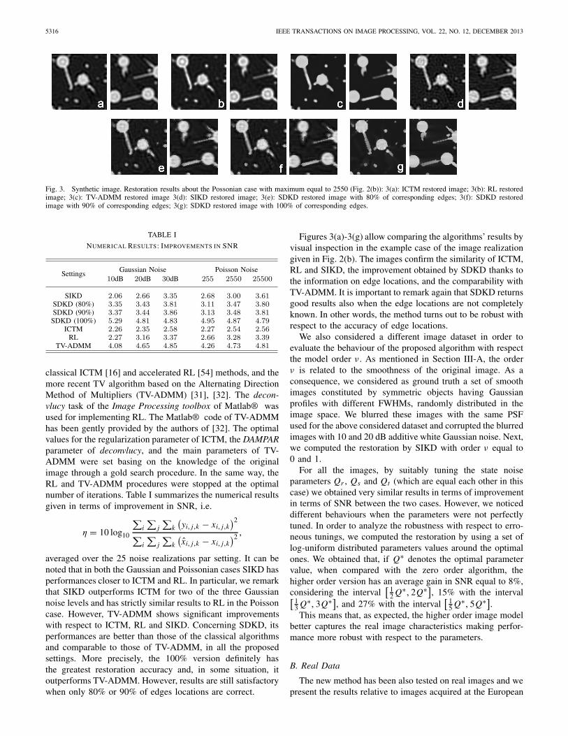
Fig. 3. Synthetic image. Restoration results about the Possonian case with maximum equal to 2550 (Fig. 2(b)): 3(a): ICTM restored image; 3(b): RL restoredimage; 3(c): TV-ADMM restored image 3(d): SIKD restored image; 3(e): SDKD restored image with 80% of corresponding edges; 3(f): SDKD restoredimage with 90% of corresponding edges; 3(g): SDKD restored image with 100% of corresponding edges.

TABLE I

NUMERICAL RESULTS: IMPROVEMENTS IN SNR

classical ICTM [16] and accelerated RL [54] methods, and themore recent TV algorithm based on the Alternating DirectionMethod of Multipliers (TV-ADMM) [31], [32]. The decon-vlucy task of the Image Processing toolbox of Matlab® wasused for implementing RL. The Matlab® code of TV-ADMMhas been gently provided by the authors of [32]. The optimalvalues for the regularization parameter of ICTM, the DAMPARparameter of deconvlucy, and the main parameters of TV-ADMM were set basing on the knowledge of the originalimage through a gold search procedure. In the same way, theRL and TV-ADMM procedures were stopped at the optimalnumber of iterations. Table I summarizes the numerical resultsgiven in terms of improvement in SNR, i.e.

η = 10 log10

∑i∑

j∑

k

(yi, j,k − xi, j,k

)2

∑i

∑j

∑k

(xi, j,k − xi, j,k

)2 ,

averaged over the 25 noise realizations par setting. It can benoted that in both the Gaussian and Poissonian cases SIKD hasperformances closer to ICTM and RL. In particular, we remarkthat SIKD outperforms ICTM for two of the three Gaussiannoise levels and has strictly similar results to RL in the Poissoncase. However, TV-ADMM shows significant improvementswith respect to ICTM, RL and SIKD. Concerning SDKD, itsperformances are better than those of the classical algorithmsand comparable to those of TV-ADMM, in all the proposedsettings. More precisely, the 100% version definitely hasthe greatest restoration accuracy and, in some situation, itoutperforms TV-ADMM. However, results are still satisfactorywhen only 80% or 90% of edges locations are correct.

Figures 3(a)-3(g) allow comparing the algorithms’ results byvisual inspection in the example case of the image realizationgiven in Fig. 2(b). The images confirm the similarity of ICTM,RL and SIKD, the improvement obtained by SDKD thanks tothe information on edge locations, and the comparability withTV-ADMM. It is important to remark again that SDKD returnsgood results also when the edge locations are not completelyknown. In other words, the method turns out to be robust withrespect to the accuracy of edge locations.

We also considered a different image dataset in order toevaluate the behaviour of the proposed algorithm with respectthe model order ν. As mentioned in Section III-A, the orderν is related to the smoothness of the original image. As aconsequence, we considered as ground truth a set of smoothimages constituted by symmetric objects having Gaussianprofiles with different FWHMs, randomly distributed in theimage space. We blurred these images with the same PSFused for the above considered dataset and corrupted the blurredimages with 10 and 20 dB additive white Gaussian noise. Next,we computed the restoration by SIKD with order ν equal to0 and 1.

For all the images, by suitably tuning the state noiseparameters Qr , Qs and Qt (which are equal each other in thiscase) we obtained very similar results in terms of improvementin terms of SNR between the two cases. However, we noticeddifferent behaviours when the parameters were not perfectlytuned. In order to analyze the robustness with respect to erro-neous tunings, we computed the restoration by using a set oflog-uniform distributed parameters values around the optimalones. We obtained that, if Q∗ denotes the optimal parametervalue, when compared with the zero order algorithm, thehigher order version has an average gain in SNR equal to 8%,considering the interval

[ 12 Q∗, 2Q∗], 15% with the interval[1

3 Q∗, 3Q∗], and 27% with the interval[ 1

5 Q∗, 5Q∗].This means that, as expected, the higher order image model

better captures the real image characteristics making perfor-mance more robust with respect to the parameters.

B. Real Data

The new method has been also tested on real images and wepresent the results relative to images acquired at the European


Fig. 4. Acquired and restored CLSM images of a specimen of mouse brain.Fig. 4(a) reports the rs- (left) and rt-views (right) of a 325 × 325 × 171voxels portion of the specimen before (top) and after (bottom) restoration.All images are Equalized Maximum Intensity Projections (MIP) of 5 slicesalong the r- and s-directions, respectively. Notice that a slight reticular textureappears in the restored images. This is due to not corrected artifacts introducedby the optical instrument, which turn out to be amplified by any deblurringprocedure. Top and central images in Fig. 4(b) are the enlargements of theMIP regions selected by the white frames in Fig. 4(a) (before (top) and after(center) restoration). The bottom image of Fig. 4(b) is a copy of the central onewhere a dendrite path is indicated by a green sign. In Fig. 4(a) the down-rightbars correspond to 80 μm for the rs-views, and 100 μm for the rt-views.

Laboratory for Non-Linear Spectroscopy (LENS) in Florence,where an improved Light-Sheet Microscopy technique, calledConfocal Light-Sheet Microscopy (CLSM), has been devel-oped [6]. The choice of CLSM images is because they arechallenging and substantially representative of other cases.It is worth noting that, since a ground truth is not available andit is therefore impossible to provide a quantitative comparisonamong different methods, the aim here is to show the impact ofdeconvolution with our approach. Indeed, we have performeddeconvolution of the same images with other methods and wedid not notice appreciable qualitative differences. However, forthe sake of completeness, we will present the result obtainedwith TV-ADMM since it was the most effective among theconsidered methods on synthetic data.

The PSF of the optical system was experimentally mea-sured by using sub-diffraction fluorescent beads. It is wellapproximated by a Gaussian fits, whose redial (r - and s-directions) and axial (t-direction) FWHM are equal to 2 and9 voxels, respectively. Figure 4 illustrates a portion of one ofthe acquired images, which is about a region of ∼700 mm3

of a mouse brain, corresponding to 1480 × 948 × 800 voxels.A 8-bit grayscale representation is used requiring about 1GB of disk space. SIKD was applied to this image withthe following parameters: ν = 0, Qr = Qs = Qt = 0.3,σv = 0.09, l = 27, d = 7. The MATLAB® implementationhas been executed by a cluster of 20 nodes (each being a 2-way quad-core Opteron 2.1GHz with 16 GB of RAM) andcompleted in 42 min.

It can be noted how the image has been generally madesharper. In particular, both neurons and dendrites have become

Fig. 5. 3-D MIP rendering of neurons and axons bundle: dimensions are233 × 185 × 240 voxels; top-left image is the volume before restoration;top-right image is the enlargement of the region selected by the white frame;down-left and -right images are the restored versions of the enlargement bySIKD and TV-ADMM (with α = 0.0015, β = 0.002 and 100 iterations),respectively. The renderings were realized using the tool Vaa3D [55].

more recognizable with respect to the image background. Thisis highlighted by Fig. 4(b) where a particular enlargement ofa 5 slice Maximum Intensity Projections (MIP) is reportedbefore (top) and after (center) restoration. It is clear hawdublurring gives the chance to follow the path of dendrites,as manually done in the bottom image by the green sign.Obviously, this is not possible by using the acquired image.

We remark that we chose to show MIP images because theeffects of deconvolution can be appreciated only using a 3-Drendering modality. This is further confirmed by Fig. 5 whichreports the 3-D MIP rendering of a different portion of thesame volume of Fig. 4. In this case, also the restoration resultsof TV-ADMM are provided. Although both the algorithms leadto an enhancement with respect to the row data and may helpin reconstructing the 3-D paths of the brain axons, they achievethis result in a different way. While SIKD produces a smoothedimage, TV-ADMM produces a slightly sharper image but withsome artifacts.

VII. CONCLUSIONS

A new denoising and deblurring algorithm for 3-Dmicroscopy images has been introduced in this paper. Theproblem is solved by applying standard Kalman filtering toan image generating model. The consistency of this model,together with the linear optimality of Kalman filter, allow themethod to provide a minimum variance linear estimation ofthe original image. The algorithm has a recursive structureand requires a unique one-shot image elaboration. Moreover,it offers the possibility to enhance the image quality byembedding the information on edge locations and to elabo-rate very large images by parallel computation. Results onsynthetic images confirm the capability of the approach interms of estimation accuracy and robustness. In particular,


the comparison with the state of the art states that the methodcan be considered as a valid alternative for the deconvolu-tion of 3-D images. Experimental results on real microscopyimages show the effectiveness of the proposed algorithm forreal frameworks.

APPENDIX A

Let us suppose that each sample of the original image xi, j,k

is governed by a given distribution with known mean valueμx . Moreover, let us define cx as cx := cm (h ∗ x)i, j,k , so that(6) becomes

vi, j,k = 1

cm(P(cx ) − cx) . (83)

The mean value and the variance of vi, j,k can be computed asE[vi, j,k ] = E

[E[vi, j,k |x

]]and σ 2

v = E[E[v2i, j,k |x]], where

E[y|x] denotes the conditional expectation of the randomvariable y conditioned to x . Recalling that E[P(c)] = c, iteasily follows that E[vi, j,k ] = 0 for all (i, j, k). By using (83)and recalling that E[P2(c)] = c + c2, it results that

σ 2v = c−2

m E[

E[(P(cx ) − cx)

2∣∣∣ x]]

= c−2m E [cx ] = c−2

m E[cm (h ∗ x)i, j,k

] = μx

cm, (84)

where the unitary volume of the PSF has been exploited. Anestimate of σ 2

v can be so obtained by (84), where μx is aparameter related to the average intensity of the original imageand cm is a characteristic of the acquisition instrumentation(e.g. CCD cameras). Notice that the noise variance decreaseswhen cm increases.

APPENDIX B

A. Components of the State Vector X (p)

The i -th component of X (p), denoted by Xi (p), is givenby

Xi (p) = ∂�x(p)

∂r�−α∂sα−λ∂ tλ

where it is easy to check that

i = φ(�, α, λ) := λ + 1

6

(�3 + 3�2 + 2�

)+ 1 + α (α + 1)

2,

and, viceversa, � = �(i), α = α(i), and λ = λ(i) satisfy

�(i) :=⎡

⎣ 3

√

3i +√

9i2 − 1

27+ 3

√

3i −√

9i2 − 1

27− 1

⎤

⎦ ,

α(i) :=[

1

2

√8i − 4

3

(�3(i) + 3�2(i) + 2�(i)

) − 7 − 1

2

],

λ(i) := i − 1

6

(�3(i) + 3�2(i) + 2�(i)

)− 1 − α2(i) + α(i)

2,

where [·] stands for the integer part.

B. Definitions of Matrices Ar , As, and At

(Ar )i, j ={

1 if j = i + θ(i) ≤ n0 otherwise

, (85)

(As)i, j ={

1 if j = i + 1 + θ(i) + α(i) ≤ n0 otherwise

, (86)

(At )i, j ={

1 if j = i + 2 + θ(i) + α(i) ≤ n0 otherwise

, (87)

where θ(i) = 1/2(�2(i) + 3�(i) + 2

).

APPENDIX C

In order to prove that the single state vector x(k) is governedby the single state equation (56) we here need to recall andintroduce some mathematical tools (details can be found in[56]).

A. Mathematical Tools

Definition 3.1 (Kronecker Product): Let M and N be realmatrices of dimensions r ×s and p ×q respectively. Then, theKronecker product M ⊗ N is defined as the (r · p) × (s · q)matrix (M ⊗ N)i, j = mi, j N , where mi, j are the entries of M .

Definition 3.2 (Matrix Stack): Let M be the r × s realmatrix

M = [m1 m2 · · · ms

],

where mi denotes the i -th column of M . Then, the stack ofM is the r · s vector

st (M) = [mT

1 mT2 · · · mT

s

]T.

It can be easily proved that the stack operator is linear.Some useful properties of the Kronecker product are:

A ⊗ (B ⊗ C) = (A ⊗ B) ⊗ C (88a)

st (A · B · C) = (CT ⊗ A) · st (B) (88b)

where A, B , C , and D are real matrices with suitable dimen-sions.

Definition 3.3: Let M ∈ R(n·r)×(n·s) and X ∈ R

(n·r)×s betwo block matrices defined by their block-entries as

M = [Mi, j

]i=1:r; j=1:s , X = [

Xi, j]

i=1:r; j=1:s ,

with Mi, j ∈ Rn×n and Xi, j ∈ R

n . Then, the product M � Xis defined as the (n · r) × s block matrix

M � X := [Mi, j Xi, j

]i=1:r; j=1:s .

When n = r = s = 1, such a product corresponds to theHadamard product [57]. Therefore, it is here referred as theBlock-Matrix Hadamard (BMH) product. Following propertiescan be proved to hold.

Lemma 3.1: Let M and X be the same matrices given inDefinition 3.3 and M be a matrix with the same structure ofM . Then, for any α, β ∈ R:

(αM + β M

)� X = α (M � X) + β

(M � X

)(89a)

st (M � X) = diagn(M) · st (X) (89b)


where diagn : R(n·r)×(n·s) → R

(n·r ·s)×(n·r ·s) is defined as

diagn(M) := diag{

Mi, j , j = 1 : l; i = 1 : l}. (90)

First property directly derives from the matrix product lin-earity. The second property can be trivially proved by directcomputing.

B. Computation of (56)

We now have the elements to derive (56). In particular, wehave to prove two conditions: 1) expressions for A(k) and B(k)in (57) and (58) hold true; 2) {w(k)} is a white Gaussian noisesequence with the covariance matrix Q(k), given in (59).

Let us recall the CE (48) at slice k + 1:

Xi, j,k+1 = ρi, j,k+1�−1i, j,k+1

(Zi, j,k+1 + Ni, j,k+1

)

+(1 − ρi, j,k+1)X0i, j,k+1.

and collect the involved quantities in the following matrices(assume i, j = 1 : l):

X(k) := [Xi, j,k

]i, j , X0(k) :=

[X0

i, j,k

]

i, j,

�(k) :=[ρi, j,k+1�−1

i, j,k+1

]

i, j, Z(k) := [

Zi, j,k+1]

i, j ,

�(k) := [(1 − ρi, j,k+1

)In]

i, j , N(k) := [Ni, j,k+1

]i, j .

By using the BMH product, defined in Definition 3.3, weeasily obtain the matricial form of the CE:

X(k + 1) = �(k)� (Z(k) + N(k))+�(k)� X0(k + 1). (91)

Next, we recognize that x(k) and x0(k), defined by (53) and(54), and quantities in (65) and (69) satisfy:

x(k) := st (X(k)) , x0(k) := st(

X0(k))

;P(k) = diagn(�(k)), T (k) = diagn(�(k));

where st and diagn are the operators defined in Definition 3.2and (90), respectively. Thus, by stacking (91) and using (89b),we get

x(k + 1) = P(k)st (Z(k) + N(k)) + T (k)x0(k + 1). (92)

Notice that last equation is similar to (56). To derive (56)from (92) we only have to develop the term st (Z(k) + N(k))as linear function of x(k) and x0(k) and collect in A(k) andB(k) their matricial coefficients, respectively, and in w(k)the remaining stochastic terms. To do this, let us define thefollowing matrices (assume here [·] = [·]i, j=1:l ):

�(μ)(k) :=[�

(μ)i, j,k+1

], �(μ)(k) :=

[�

(μ)i, j,k+1

],

Z(μ)(k) :=[�

(μ)i, j,k+1 Z (μ)

i, j,k+1

], W(μ)(k) :=

[W (μ)

i, j,k+1

],

N(μ)(k) :=[�

(μ)i, j,k+1 N (μ)

i, j,k+1

], W0(k) :=

[W 0

i, j,k+1

],

�(μ)(k) := �(μ)

(k) + �(μ)

(k);and recognize that (66)-(68) satisfy O(k) = diagn(�

(μ)(k)),O(k) = diagn(�

(μ)(k)), and O(k) = diagn(�(μ)(k). Using

(50), we can write that

st (Z(k) + N(k)) =5∑

μ=1

st(

Z(μ)(k))

+5∑

μ=1

st(

N(μ)(k))

.

with:

st(

Z(1)(k))

= O(1)(k)(Il2 ⊗ H1

)x(k), (93a)

st(

Z(2)(k))

= O(2)(k) ((Tl ⊗ Il ) ⊗ H2 H1) x(k)

+ O(2)(k) ((Tl ⊗ Il ) ⊗ H2) x0(k + 1), (93b)

st(

Z(3)(k))

= O(3)(k) ((Il ⊗ Tl ) ⊗ H3 H1) x(k)

+ O(2)(k) ((Il ⊗ Tl ) ⊗ H3) x0(k + 1), (93c)

st(

Z(4)(k))

= O(4)(k) ((Sl ⊗ Il ) ⊗ H4 H1) x(k)

+ O(4)(k) ((Sl ⊗ Il ) ⊗ H4) x0(k + 1), (93d)

st(

Z(5)(k))

= O(5)(k) ((Il ⊗ Sl) ⊗ H5 H1) x(k)

+ O(5)(k) ((Il ⊗ Sl) ⊗ H5) x0(k + 1), (93e)

st(

N(1)(k))

= O(1)(k)w(1)(k), (93f)

st(

N(2)(k))

= O(2)(k) ((Tl ⊗ Il ) ⊗ H2) w(1)(k)

+ O(2)(k) ((Tl ⊗ Il ) ⊗ H2) w0(k) + O(2)(k)w(2)(k), (93g)

st(

N(3)(k))

= O(3)(k) ((Il ⊗ Tl ) ⊗ H3) w(1)(k)

+ O(3)(k) ((Il ⊗ Tl ) ⊗ H3) w0(k) + O(3)(k)w(3)(k), (93h)

st(

N(4)(k))

= O(4)(k) ((Sl ⊗ Il ) ⊗ H4) w(1)(k)

− O(4)(k) ((Sl ⊗ Il ) ⊗ H4) w(2)(k)

+ O(4)(k) ((Sl ⊗ Il ) ⊗ H4) w0(k), (93i)

st(

N(5)(k))

= O(5)(k) ((Il ⊗ Sl) ⊗ H5) w(1)(k)

− O(5)(k) ((Il ⊗ Sl) ⊗ H5) w(3)(k)

+ O(5)(k) ((Il ⊗ Sl) ⊗ H5) w0(k). (93j)

where

w(μ)(k) := st(

W(μ)(k))

, w0(k) := st(

W0(k))

, (94)

for μ = 1 : 5. A sketch proof of (93a)–(93j) is given inAppendix C-C. The substitution of st (Z(k) + N(k)) into (92),taking into account (93a)–(93j), finally proves both conditions1) and 2). Indeed, let us focus on condition 1): equations(57) and (58) can be readily derived as sum of the matricialcoefficients of x(k) and x0(k + 1) in (92) and (93a)-(93e),respectively. As far as condition 2) is concerned, the randomvector w(k) is defined by collecting all remaining stochasticterms:

w(k) := F0(k)w0(k) +3∑

μ=1

Fμ(k)w(μ)(k), (95)

where it is easy to verify that Fμ(μ = 0 : 3) actu-ally correspond to (60)-(63). Moreover, taking into account(18)–(21), together with property (30), from (94) follows thatsequences

{w0(k)

}and

{w(μ)(k)

}(μ = 1, 2, 3) are white,

Gaussian, zero-mean and independent each others. They also


satisfy

E

[w0(k)

(w0(k)

)T]

= δk,k Q0,

E[w(μ)(k)w(μ)T (k)

]= δk,k Qμ,

where Q0 and Qμ (μ = 1, 2, 3) are the matrices definedin (64). As a consequence, from (95) we have that w(k) isGaussian and, for any k, k = 1 : H :

E [w(k)] = 0, E[w(k)wT (k)

]= δk,k Q(k),

where Q(k) satisfies (59). This corresponds to condition 2).

C. Proof of (93a)–(93j)

Equations (93a)–(93j) can be obtained by taking intoaccount the definition of Z (μ)

i, j,k(k) and N (μ)i, j,k (k), given accord-

ing to (33), relations (23), (24) and (37), and using properties(88a) (88b), (89a), and (89b).

We here prove (93a). Consider that vectors composingmatrix Z(1)(k) have the form �

(1)i, j,k+1 Z (1)

i, j,k+1. By substituting

the expression of Z (1)i, j,k+1 in (34), and taking into account (37)

and then (43), we have:

�(1)i, j,k+1 Z (1)

i, j,k+1 = �(1)i, j,k+1 Xi, j,k = �

(1)i, j,k+1 H1Xi, j,k .

Recalling the definition of the BMH product �, we have:

Z(1)(k) = �(1)

(k) �

⎡

⎢⎣H1X1,1,k · · · H1X1,l,k

.... . .

...H1Xl,1,k · · · H1Xl,l,k

⎤

⎥⎦

= �(1)

(k) � [(Il ⊗ H1) X(k)] .

Next, applying (89b) to last equation, we get:

st(

Z(1)(k))

= diagn

(�

(1)(k)

)st ((Il ⊗ H1) X(k)) ,

from which:

st(

Z(1)(k))

= diagn

(�

(1)(k)

)st ((Il ⊗ H1) X(k)Il)

(Pr. (88b)) = diagn

(�

(1)(k)

)(Il ⊗ (Il ⊗ H1)) st (X(k))

(Pr. (88a)) = O(1)(k)(Il2 ⊗ H1

)x(k),

which corresponds to (93a). The remaining (93b)–(93j) can beobtained in a similar way.

ACKNOWLEDGEMENTS

The authors thank Valeria Ruggiero, Gaetano Zanghiratiand the anonymous referees for their helpful suggestions inrevising the manuscripts.

REFERENCES

[1] P. Sarder and A. Nehoray, “Deconvolution methods for 3-D fluores-cence microscopy images,” IEEE Signal Process. Mag., vol. 23, no. 3,pp. 32–45, May 2006.

[2] J. B. Pawley, Handbook of Biological Confocal Microscopy. New York,NY, USA: Springer-Verlag, 2006.

[3] E. H. K. Stelzer and S. Lindek, “Fundamental reduction of the obser-vation volume in far-field light microscopy by detection orthogonalto the illumination axis: Confocal theta microscopy,” Opt. Commun.,vol. 111, nos. 5–6, pp. 536–547, 1994.

[4] A. H. Voie, “Imaging the intact guinea pig tympanic bulla byorthogonal-plane fluorescence optical sectioning microscopy,” Hear.Res., vol. 171, nos. 1–2, pp. 119–128, 2002.

[5] J. Huisken, J. Swoger, F. D. Bene, J. Wittbrodt, and E. Stelzer, “Opticalsectioning deep inside live embryos by selective plane illuminationmicroscopy,” Science, vol. 305, pp. 1007–1009, Aug. 2004.

[6] L. Silvestri, A. Bria, L. Sacconi, G. Iannello, and F. S. Pavone,“Confocal light sheet microscopy: Micron-scale neuroanatomy of theentire mouse brain,” Opt. Exp., vol. 20, no. 18, pp. 20582–98, 2012.

[7] P. J. Keller and H.-U. Dodt, “Light sheet microscopy of livingor cleared specimens,” Current Opinion Neurobiol., vol. 22, no. 1,pp. 138–143, 2012.

[8] A. Tsai, A. J. Yezzi, and A. Willsky, “Curve evolution implementationof the Mumford-Shah functional for image segmentation, denoising,interpolation, and magnification,” IEEE Trans. Image Process., vol. 10,no. 8, pp. 1169–1186, Aug. 2001.

[9] H. Jin, Y. H. T. A. J. Yezzi, L. T. Cheng, and S. Soatto, “Estimationof 3D surface shape and smooth radiance from 2D images: A level setapproach,” J. Sci. Comput., vol. 19, nos. 1–3, pp. 267–292, 2003.

[10] J. Swoger, P. Verveer, K. Greger, J. Huisken, and E. Stelzer,“Multi-view image fusion improves resolution in three-dimensionalmicroscopy,” Opt. Exp., vol. 15, no. 13, pp. 8029–8042, 2007.

[11] H. Adorf, R. Hook, and R. Lucy, “HST image restoration developmentsat the ST-ECF,” Int. J. Imag. Syst. Technol., vol. 6, no. 4, pp. 339–349,1995.

[12] A. Jalobeanu, L. Blanc-Féraud, and J. Zerubia, “An adaptive Gaussianmodel for satellite image deblurring,” IEEE Trans. Image Process.,vol. 13, no. 4, pp. 613–621, Apr. 2004.

[13] T. Tomasi, A. Diaspro, and B. Bianco, “3-D reconstruction in opticalmicroscopy by a frequency-domain approach,” Signal Process., vol. 32,no. 3, pp. 357–366, 1993.

[14] A. Tikhonov and V. Arsenin, Solutions of Ill-Posed Problems. NewYork, NY, USA: Wiley, 1977.

[15] C. Preza, M. I. Miller, L. J. Thomas, Jr., and J. G. McNally, “Regular-ized linear method for reconstruction of three dimensional microscopicobjects from optical sectioning,” J. Opt. Soc. Amer. A, vol. 9, no. 2,pp. 219–228, 1992.

[16] H. van der Voort and K. Strasters, “Restoration of confocal images forquantitative image analysis,” J. Microsc., vol. 179, no. 2, pp. 165–181,1995.

[17] W. Carrington, R. Lynch, E. Moore, G. Isenberg, K. Fogarty, andF. Fay, “Superresolution three-dimensional images of fluorescencein cells with minimal exposure,” Science, vol. 268, pp. 1483–1487,Jun. 1995.

[18] G. van Kempen and L. van Vliet, “The influence of the regularizationparameter and the first estimate on the performance of Tikhonov regu-larized non-linear image restoration algorithm,” J. Microsc., vol. 198,no. 1, pp. 63–75, 2000.

[19] T. Holmes, “Maximum-likelihood image restoration adapted for non-coherent optical imaging,” J. Opt. Soc. Amer. A, vol. 5, no. 5,pp. 666–673, 1988.

[20] M. Bertero and P. Boccacci, “A simple method for the reduction ofboundary effects in the Richardson-Lucy approach to image deconvo-lution,” Astron. Astrophys., vol. 437, no. 1, pp. 369–374, 2005.

[21] J.-A. Conchello and J. C. McNally, Fast Regularization Tech-nique for Expectation Minimization Algorithm for Optical SectioningMicroscopy, vol. 2655, C. J. Cogswell, G. S. Kino, and T. Wilson, Eds.San Jose, CA, USA: SPIE, 1996, pp. 199–208.

[22] P. Verveer and T. Jovin, “Efficient super resolution restoration algo-rithms using maximum a posteriori estimations with application to flu-orescence microscopy,” J. Opt. Soc. Amer. A, vol. 14, no. 8, pp. 1696–1706, 1997.

[23] M. A. T. Figueiredo and R. Nowak, “An EM algorithm for wavelet-based image restoration,” IEEE Trans. Image Process., vol. 12, no. 8,pp. 906–916, Aug. 2003.

[24] L. Rudin, S. Osher, and E. Fatemi, “Nonlinear total variation basednoise removal algorithms,” Phys. D, Nonlinear Phenomena, vol. 6,no. 1, pp. 259–268, 1992.

[25] N. Dey, L. Blanc-Feraud, C. Zimmer, P. Roux, Z. Kam, J.-C. Olivo-Marin, et al., “Richardson-Lucy algorithm with total variation regu-larization for 3D confocal microscope deconvolution,” Microsc. Res.Tech., vol. 69, no. 4, pp. 260–266, 2006.

[26] J. Dahl, P. Hansen, S. Jensen, and T. Jensen, “Algorithms and softwarefor total variation image reconstruction via first-order methods,” Numer.Algorithms, vol. 53, no. 1, pp. 67–92, 2010.


[27] S. Bonettini and V. Ruggiero, “An alternating extragradient methodfor total variation based image restoration from Poisson data,” InverseProblems, vol. 27, no. 9, pp. 095001-1–095001-26, 2011.

[28] R. Nowak and M. Thul, “Wavelet-vaguelette restoration in photon-limited imaging,” in Proc. IEEE Int. Conf. Acoust., Speech, SignalProcess., vol. 5. May 1998, pp. 2869–2872.

[29] T. Goldstein and S. Osher, “The split Bregman method for L1 regu-larized problems,” Dept. Comput. Appl. Math., Univ. California, LosAngeles, CA, USA, Tech. Rep. 08-29, 2008.

[30] M. A. T. Figueiredo and J. M. Bioucas-Dias, “Restoration of Poissonianimages using alternating direction optimization,” IEEE Trans. ImageProcess., vol. 19, no. 12, pp. 3133–3145, Dec. 2010.

[31] S. Setzer, G. Steidl, and T. Tueber, “Deblurring Poissonian images bysplit Bregman techinques,” J. Vis. Commun. Image Represent., vol. 21,no. 3, pp. 193–199, 2010.

[32] F. de Vieilleville, P. Weiss, V. Lobjois, and D. Kouame, “Alternatingdirection method of multipliers applied to 3D light sheet fluorescencemicroscopy image deblurring using GPU hardware,” in Proc. Annu.Int. Conf. IEEE EMBC, Aug./Sep. 2011, pp. 4872–4875.

[33] H. Trussel and B. Hunt, “Improved methods of maximum a posteriorirestoration,” IEEE Trans. Comput., vol. 27, no. 1, pp. 57–62, Jan. 1979.

[34] G. R. Ayers and J. C. Dainty, “Iterative blind deconvolution methodand its applications,” Opt. Lett., vol. 13, no. 7, pp. 547–549, Jul. 1988.

[35] V. Krishnamurthi, Y. H. Liu, S. Bhattacharyya, J. N. Turner, andT. J. Holmes, “Blind deconvolution of fluorescence micrographsby maximum-likelihood estimation,” Appl. Opt., vol. 34, no. 29,pp. 6633–6647, 1995.

[36] G. B. Avinash, “Simultaneous blur and image restoration in 3D opticalmicroscopy,” Zool. Stud., vol. 34, no. 1, pp. 184–185, 1995.

[37] D. A. Fish, A. M. Brinicombe, E. R. Pike, and J. C. Walker, “Blinddeconvolution by means of the Richardson-Lucy algorithm,” J. Opt.Soc. Amer. A, vol. 12, no. 1, pp. 58–65, 1995.

[38] J. Markham and J. Conchello, “Parametric blind deconvolution:A robust method for the simultaneous estimation of image and blur,”J. Opt. Soc. Amer. A, vol. 16, no. 10, pp. 2377–2391, 1999.

[39] A. Germani and L. Jetto, “Image modeling and restoration: A newapproach,” Circuits Syst. Signal Process., vol. 7, no. 4, pp. 427–457,1988.

[40] A. De Santis, A. Germani, and L. Jetto, “Space-variant recursiverestoration of noisy images,” IEEE Trans. Circuits Syst. II, AnalogDigit. Signal Process., vol. 41, no. 4, pp. 249–261, Apr. 1994.

[41] M. Dalla Mora, A. Germani, and A. Nardecchia, “Restoration of imagescorrupted by additive non-Gaussian noise,” IEEE Trans. Circuits Syst.II, Analog Digit. Signal Process., vol. 48, no. 7, pp. 859–875, Jul. 2001.

[42] L. Jetto, “Stochastic modelling and 3D minimum variance recursiveestimation of image sequences,” Multidimensional Syst. Sign. Process.,vol. 10, no. 3, pp. 225–254, 1999.

[43] A. De Santis, A. Germani, and L. Jetto, Space-Variant Two-Dimensional Filtering of Noisy Images, vol. 119. San Francisco, CA,USA: Academic, 2001, pp. 267–318.

[44] F. Conte, A. Germani, and G. Iannello, “A new approach for decon-volution and filtering of 3-D microscopy images,” in Proc. IFAC WC,Dec. 2011, pp. 1180–1185.

[45] J. McNally, T. Karpova, J. Cooper, and J. Conchello, “Three-dimensional imaging by deconvolution microscopy,” Methods, vol. 19,no. 3, pp. 373–385, 1999.

[46] M. Temerinac-Ott, O. Ronneberger, P. Ochs, W. Driever, T. Brox, andH. Burkhardt, “Multiview deblurring for 3-D images from light sheetbased fluorescence microscopy,” IEEE Trans. Image Process., vol. 21,no. 4, pp. 1863–1873, Apr. 2012.

[47] D. Marr and E. Hildreth, “Theory of edge detection,” Proc. R. Soc.London, Series B, Biol. Sci., vol. 207, no. 1167, pp. 187–217, 1980.

[48] J. F. Canny, “A computational approach to edge detection,” IEEETrans. Pattern Anal. Mach. Intell., vol. PAMI-8, no. 6, pp. 679–698,Nov. 1986.

[49] A. K. Jain, Foundamentals of Digital Image Processing. EnglewoodCliffs, NJ, USA: Prentice-Hall, 1989.

[50] B. Jähne, Digital Image Processing. Berlin-Heidelberg, Germany:Springer-Verlag, 2002.

[51] A. Balakrishnan, Kalman Filtering Theory. New York, NY, USA:Optimization Software, Inc., 1984.

[52] M. Bertero and P. Boccacci, Introduction to Inverse Problems inImaging. New York, NY, USA: Taylor & Francis, 1998.

[53] (2013). 3-D Kalman Deconvolution Toolbox [Online]. Avail-able: http://www.iconfoundation.net/content/3d-kalman-deconvolution-toolbox

[54] D. S. C. Biggs and M. Andrews, “Acceleration of iterative imagerestoration algorithms,” Appl. Opt., vol. 36, no. 8, pp. 1766–1775, 1997.

[55] H. Peng, Z. Ruan, F. Long, J. H. Simpson, and E. W. Myers, “V3Denables real-time 3D visualization and quantitative analysis of large-scale biological image data sets,” Nature Biotechnol., vol. 28, no. 4,pp. 348–353, 2010.

[56] F. Carravetta, A. Germani, and M. Raimondi, “Polynomial filtering forlinear discrete time non-Gaussian systems,” SIAM J. Control Optim.,vol. 34, pp. 1666–1690, Sep. 1996.

[57] R. A. Horn and C. R. Johnson, Topics in Matrix Analysis. Cambridge,U.K.: Cambridge Univ. Press, 1991.

Francesco Conte received the master’s degree incomputer science and automatic engineering andthe Ph.D. degree in electrical and information engi-neering from the University of L’Aquila, L’Aquila,Italy, in 2009 and 2013, respectively. He currentlyis a Post-Doctoral Fellow at the Intelligent ElectricEnergy Systems Laboratory, DITEN, University ofGenova, Genova, Italy. From 2008 to 2009, he wasa Visiting Scholar with the French National Institutefor Research in Computer Science and Control,Grenoble, France. His areas of interest include non-

linear and non-Gaussian filtering, nonlinear control theory, image processingand restoring, power system modelling and control, and mobile robotics. Theresults of the scientific work were presented in more than ten publications ininternational journals and conferences.

Alfredo Germani received the Laurea degree inphysics and the Post-Doctoral degree in computerand system engineering from the University of RomeLa Sapienza, Rome, Italy, in 1972 and 1974, respec-tively. From 1975 to 1986, he was a Researcherat Istituto di Analisi dei Sistemi e Informatica A.Ruberti, Italian National Research Council, Rome.In 1978 and 1979, he was a Visiting Scholar withthe Department of System Science, University ofCalifornia at Los Angeles, Los Angeles, CA, USA.From 1986 to 1987, he was a Professor of automatic

control at the University of Calabria, Calabria, Italy. Since 1987, he hasbeen a Full Professor of system theory at University of L’Aquila, L’Aquila,Italy, from 1989 to 1992, he has been the Chairperson of the School ofElectronic Engineering. At the University of L’Aquila, he lead the Departmentof Electrical Engineering, from 1995 to 2000, and he has been the Coordinatorof the Ph.D. School in Electronics from 1996 to 2009. Since 2001, he has beena member of the Executive Committee of the Research Center of Excellence(DEWS) and he has been a member of the advisory board of the EngineeringSchool since 2007. His areas of interest include systems theory, systemsidentification and data analysis, nonlinear, stochastic and optimal controltheory, distributed and delay systems, finitely additive white noise theory,approximation theory, optimal polynomial filtering for non-Gaussian systems,image processing and restoring, and mathematical modeling for biologicalprocesses.

Giulio Iannello received the Degree in electronicengineering from Politecnico di Milano, Milano,Italy, in 1981, and the Ph.D. degree in computerscience and computer engineering from the Univer-sity of Napoli Federico II, Napoli, Italy, in 1987.Currently, he is a Full Professor of computer scienceand computer engineering at the University CampusBio-Medico di Roma, Rome, Italy, where he is theCoordinator of the Ph.D. Program in biomedicalengineering and is responsible for the ResearchGroup on computer systems and bioinformatics.

His current research interests include biomedical and biological data, signaland image processing, multimedia data processing, bioinformatics, wirelessand high performance computer networks, design and analysis of parallelalgorithms, and performance evaluation of parallel and distributed systems.He has published over 120 journal and conference papers. He is a memberof several Program Committees of International Conferences and referee ofInternational Journals. Dr. Iannello is a member of the ACM and GIRPR.

本文献由“学霸图书馆-文献云下载”收集自网络，仅供学习交流使用。

学霸图书馆（www.xuebalib.com）是一个“整合众多图书馆数据库资源，

提供一站式文献检索和下载服务”的24 小时在线不限IP

图书馆。

图书馆致力于便利、促进学习与科研，提供最强文献下载服务。

图书馆导航：

图书馆首页文献云下载图书馆入口外文数据库大全疑难文献辅助工具

http://www.xuebalib.com/cloud/

http://www.xuebalib.com/

http://www.xuebalib.com/cloud/


http://www.xuebalib.com/vip.html

http://www.xuebalib.com/db.php

http://www.xuebalib.com/zixun/2014-08-15/44.html


5306 IEEE TRANSACTIONS ON IMAGE PROCESSING, VOL. …download.xuebalib.com/xuebalib.com.48932.pdf ·...

Documents

Transcript of 5306 IEEE TRANSACTIONS ON IMAGE PROCESSING, VOL. …download.xuebalib.com/xuebalib.com.48932.pdf ·...