517 THE EULER-BERNOULLI BEAN EQUATION WITH BOUNDARY ENERGY ... · PDF fileAD-RIBS 517 THE...
34
AD-RIBS 517 THE EULER-BERNOULLI BEAN EQUATION WITH BOUNDARY ENERGY 1/1 DISSIPATION(U) PENNSYLVANIA STATE UNIV UNIVERSITY PAMK 0 CHEN ET AL. 65 JAN 89 RFOSR-TR-09-9147 RFOSR-95-0253 UNCLSSIFIEDF G /0 9/1NL I fflfflfflfflfmfllfl LK"
-
Upload
truongxuyen -
Category
Documents
-
view
237 -
download
4
Transcript of 517 THE EULER-BERNOULLI BEAN EQUATION WITH BOUNDARY ENERGY ... · PDF fileAD-RIBS 517 THE...

AD-RIBS 517 THE EULER-BERNOULLI BEAN EQUATION WITH BOUNDARY ENERGY 1/1DISSIPATION(U) PENNSYLVANIA STATE UNIV UNIVERSITY PAMK0 CHEN ET AL. 65 JAN 89 RFOSR-TR-09-9147 RFOSR-95-0253
UNCLSSIFIEDF G /0 9/1NL
I fflfflfflfflfmfllfl
LK"

p
•,-.-
4.
0.','-'.+
.. 50 9,
u i . ? ; , .
l,, WI..__,
j 0
N". - Z -"
-. 3.3
,..- .,-
+ + + + 9 . . .1*+

1b..
I.REPO0RT SfCURITY CLA AD-A 189 517 EATRICIN MARGunclassified
-24 SECURITY CLASSIFICATION AUTHORITY 3 DISTRIBUTION/ AVAILABILITY OF REPORTP'
21:1. DECLASSIFICATION/DOWI4GRAOING SCHEDULE App1sti but' oil U uniied*.:
*PERFORMING ORGANIZATION REPORT NUMBER(S) S5 MONITORING ORGANIZATION REPORT NUMBER(S)
60. NAME OF PERFORMING ORGANIZATION 6b OFFICE SYMBOL 7a NAME OF MONITORING ORGANIZATIONV
Pennsylvania State University AORN6c. ADDRESS (Cry, Stat, and ZIP Code) 7b AIOSSQt Stae,. and ZIP Code)
University Park, PA 16802 BldgApc 203324 %
Sm. NAME OF FUNDING/ SPONSORING 6b. OFFICE SYMBOL 9 PROCUREMENT INSTRUMENT iDENTIFiCATI ft.'
%%.W)3JW4ly, State, and ZIP Co*t) 10 SOURCE OF FUNDING NUMBERSPROGRAM IPROJECT jTASK WORK UNITBldg 410 ELMN O Io NO. JACCESSION NO
Belling A1B DC 20332-848WSl I11. TITLE (Include Seaamy" QaInhEeSfon)
The Euler-.Bernoulli Beam Equation with Boundary Energy Dissipation
12. PERSONAL AUITHOR(S)
G. Chen., S.C. Krantz, D.W. Ma, C.E. Wayne, H.H. West
Paver in Book TRO 3b IM 85RE 14. DATE O ECR erjitl0y I.PCO~N13. YE FREOR 1.TIM 1/85R TO83/
7 19881 Dy ,5 CON
16. SUPPL.EMENTARY NOTATION
FICEATLCDE 18 SUBJECT TERMS (Cornie an rover"e if nftceary and identify by b61c0 numbe,)IED GROUP SUE-GROUP
19 ABSTRACT (Caoinlue an ieverse of noceinary and idenrtifly by bloc* number)Many problems in structural dynamics involve stabilizing the Euler-Bernoulli beam
equation by proportional dissipative control at the end of the beam. The COFS experiment by..NIASA is one of such examples. Exponential stability is a very desirable property for suchelastic systems. Existing methods such as the energy multiplier method have been successful
to stalis rioros poof fo cetai tpes of stabilizing boundary conditions. But thereare many other types of boundary conditions for which such methods are not effective.
A recent theorem due to F.L. Huang introduces a frequency domain method to study theexponential stability problems. Here we apply Huang's theorem to prove an exponential decayresult for an Euler-Bernoulli beam with race control of the bending moment only. We are alsoable to derive- its asymptotic stability margin. Finally, we indicate the realizability ofvarious types of boundary feedback stabilization schemes by illustrating the correspondingmechanical designs of passive damping devices.
20. 01SThOIUTION IAVAILABILITY OF ABSTRACT V1. ABSTILACT SECURITY CLASSIFICATIONMUNCLASSIFIED1UNLIMITED 03 SAME AS tP? Q3 OTiC USERS
124. NAME Of RESPONSIBLE INDIVIDUAL 22b. TELEPHONE (Include Amea Code) 22C. QEJICE SYMBOLDr. Richard K. Miller 20 6752
DOFOM 173.~u~ B3A~e~onmv~ese~utI~sha~~.SECjRtty CLASSIFICATION OF -HIS PAGEAll other edition% are oblioliote.
%..

AFOB.ThI . 88-0 147
The Euler-Bernoulli Beam Equationwith Boundary Energy Dissipation
G. Chen, S.G. Krantz*, D.W. Ma, C.E. WayneDepartment of Mathematics
The Pennsylvania State UniversityUniversity Park, Pennsylvania
H.H. WestDepartment of Civil EngineeringPennsylvania State UniversityUniversity Park, Pennsylvania
INTRODUCTION %
'Many problems in structural dynamics involve stabilizing the elasticenergy of partial differential equations such as the Euler-Bernoulli Pbeam equation by boundary conditions. Exponential stability is a very
desirable property for such elastic systems. The energy multiplier
method "-Fj-4h-- -f'has been successfully applied by several people toestablish exponential stability for various PDEs and boundary conditions.
However, it has also been found_12]'that for certain boundary conditions
the energy multiplier method Is not effective in proving the exponential
stability property.
A recent theorem of F.L. Huang 14] introduces a frequency domain
method to study such exponential decay problems. In this paper, wederive estimates of the resolvent operator on the imaginary axis and
apply Huang's theorem to establish an exponential decay result for an
Euler-Bernoulli beam with rate control of the bending moment only. We
also derive asymptotic limits of eigenfrequencles. which was also done
earlier by P. Rideau.[8]) Finally, we indicate the realizability of
these boundary feedback stabilization schemes by illustrating some
mechanical designs of passive damping devices. W
/1
II
*Current affiliation: Washington University, St. Louis, Missouri
Supported in part by NSF Grants DMS 84-01297A01. 85-01306, 84-03664 and
AFOSR Grant 85-0253. The U.S. Government is authorized to reproduce and
distribute reprints for governmental purposes notwithstanding any
copyright notation thereon.
67
88 2 26 125

68 Chen, et al.
§I. BACKGROUND AND MOTIVATION
In this paper, we consider the following uniform Euler-Bernoulli beamequation with dissipative boundary conditions
mytt(x.t)*EIyxx(xt) -0. 0 < x < 1V(0.t) -0.Yx(0 t) - 0.
-ElYxx(l.t) = -k Yt(1.t) . kk 2 3.-EZxxi') kyxtlZt) k2 e R.
(y(x,O),yt(x,0)) - (Yo(X),Yl(X)), 0 S x S I.
where m denotes the mass density per unit length, El is the flexuralrigidity coefficient, and the following variables have engineering
meanings:
y = vertical displacement. yt- velocity
Y= rotation, Yxt - angular velocity
=-Elyx bending moment
-EIYxxx = shear
at a point x, at time t.From now on. when we write equation (1.l.J), for example, we mean p
the Jth equation in (1.1).The above equation and conditions are Intended to serve as a simple
mathematical model for the mast control system in NASA's COFS (Control
of Flexible Structures) Program. See Figure 1. A long flexible mast 60meters in length is clamped at its base on a space shuttle. The mast isformed with 54 bays but can be idealized as a continuous uniform beam.
At the very end of the mast, a CMG (control moment gyro) is placed which
can apply bending and torsion rate control to the mast according to
sensor feedback.
Boundary conditions (1.1.2) and (1.1.3) signify that the beam is
clamped, at the left end, x = 0. while boundary conditions (1.1.4) and
(1.1.5) at the right end, x = 1, respectively, signify
Ishear (-Elyxxx) is proportional to velocity (yt}
bending moment (-EIyxx) is negatively proportional to angular
velocity (Yxt)
Thus the rate feedback laws (1.1.4) and (1.1.5) reflect some basic
features of the CMG mast control system In COFS.
7r%4
W4

Euler-Bernoulli Beam Equation 69
CMG
flexible ma3st
L space shuttle
Flure 1 Spacecraft mast control experiment
The elastic energy of vibration. E(t), at time t. for system
(1.1) is given by
EM a I f0 (my2(x.t) xt)Jdx ,.
Note that In (1.1) we have already normalized the beam length to 1.
The qualitative behavior of (1.1) has been studied in an earlier
paper [2]. There it is shown that if k2 > 0. k > 0 in (1.1.4) and ,
(1.1.5). respectively, then the energy of vibration of the beam decays .
uniformly exponentially: |
Et) < Ke-PtE(O) (1.2)
for some K,p > 0 uniformly for all initial conditions (yo(x).yl(x)). A
Therefore the flexible mast system can be controlled and stabilized.
The proof of the above In (2] was accomplished by the use of energy
multipliers and the construction of a Liapounov functional.
Nevertheless, a major mathematical question remained unresolved in (2]:
(Q] "Does the uniform exponentinl decay property (1.2) hold under the. Accession For
assumption of k2 .0o, k2 > 0?" NTIS CFA&I2DTIC T,..Unale' ouaneed
This question is of considerable mathematical Interest because the Juitification
feedback scheme using bending moment only is simple and attractive.
ByDistribution/
AvailabIlitv CodeS
Av ;.± anid/or''Cist Special
S% %..6%C.

70 Chen, et &I.
For a long time, we have conjectured that the answer to [Q) is
affirmative, as asymptotic elgenfrequency estimates obtained in (8] (and§3) have so suggested: Let A denote the Infinitesimal generator of
the CO-semigroup corresponding to (1.1) with k1 = 0 and k2 > 0, and
let a(A) denote the spectrum of A. Then there exists P > 0 such that
Re X S -P < 0 for all X e o(A). (1.3)
Nevertheless, It is well known (41 that the following "theorem" is
false. 4"Let A generate a Co-semigroup and
sup(Re N E o(A)) -P < 0 (1.4)
for some P > 0. Then the Co-semigroup is exponentially stable:
Jlexp(tA)IJ < Me-# t for some M > 1, p > 0". (1.5)
Therefore, knowing (1.4) alone is not sufficient to confirm (1.5). This
statement remains false even if we assume additionally that A has a
compact resolvent. I
We have repeatedly tried to refine the energy multiplier technique , 4
used in (2] to establish (1.5) without much success, no matter how manydifferent and elaborate multipliers were constructed. There always are
boundary terms which cannot be absorbed by terms in the dissipative ,P
boundary condition.
A recent theorem by P.L. Huang offers an important direct method
for proving exponential stability:
THEOREM 1 (F.L. Huang f41)
Let exp(tA) be a Co-semigroup In a Hilbert space satisfying
lexp(tA)II < B0 1 t > 0. for some B0 > 0. (1.6)
Then exp(tA) is exponentially stable if and only if
(Iwcj E R ) C p(A), the resolvent set of A; and (1.7)
B1 sup(II(i-A)- lll" e R) < - (1.8)
%
I)
I,%'. .. . . . . . . V'.I
.< . , . .,. .,.,. ,,... < -.- % :.7 - / /;* :

Euler-Bernoulli Beam Equation 71
are satisfied. 0
Huang's theorem effects a frequency domain method to proving
exponential decay properties. As mentioned earlier, the energy
multiplier method, which corresponds to a time domain method, has not
been successful for the case k2 . 0, > 0.
Therefore the work is to obtain bounds on the resolvent operator
(Iw-A)- 1 . Here we accomplish this by carrying out a careful analysis
on the elgenfunctlons and elgenfrequencles of the operator A. This Is
done In §2.
Associated with [Q] is the question of the asymptotic distribution
pattern of elgenfrequencies. as numerical study In [2) suggests that a P,
"structural damping" phenomenon Is present at low frequencies. Does it
also appear at high frequencies? This is answered in §3. (We must statethat the work and numerical verification was done ahead of us by P.
Rideau in his recent thesis (8]).
In §4. we present mechanical designs of devices satisfying dampingboundary conditions (1.1.3) and (1.1.4) to indicate the realizability
of the feedback stabilization scheme using passive dampers,
Notations: We use II to denote the 12(0.1) norm. We define the S r
Sobolev space
k
Nk a H k (0 1 ) - (f:[OlJ.*RIfll 2 a XfO1if(j)(x)I2dx < -), k E N.Hk(O.1) J'*0
Also, we let
2 a H2(0.1) n (fi G H2(0,1), f(O) - f'(0) - 0).
The underlying Hilbert space I for the PDE (1.1) is
14 .2 (0 )XZ2 2 ,* 1 *() 2 .M gx 2H0 (0, (0.1) .1 ((f.g)lll(f.g)ll • f 0 [Eilf"(x)1 mlglx)1 dx<-).
whose norm square is the elastic energy.The unbounded linear operator A associated with (1.1) is given by
A _4a4 --
4%
"po'7:S7
WM -7V fob? I It,,' *

72 Chen, et al.
with domain
D (A) •((r.g) IE H4xH21 I - "' ( l ) = - k 2 g ( 1) . - E I f ''" = 2 g ( 1 ~ } t (I) -k0
J2. ESTIKA'fION OF THE RESOLVENT OPERATOR ON THE IMAGINARY AXIS.
EXPONENTIAl. DECAY OF SOLUTIONS.
Consider the resolvent equation: Given (f.g) e If and X E C, find
(w).,v) G D(A) such that
A ,I - ( 4 - (2.1)- , 3 2-1) o J [
This amounts to solving the following boundary value problem for w.:
4w(4x ) + X2w(x) = -[Xf(x)g(x)lj, x E (0.1)
w(O) - 0
W (O) *0 (2.2)w() (1) -f(i)
W"w~(1) .,) _f,)
where
;2 k2(EI-', k2 uk 2 (EI)-1 231 2 2 2 1(23
Once wA is found we obtain
vX(x) - Awx(x) * f(x) (2.4)
To simplify notation, from now on. unless otherwise specifically
mentioned, we set 04 1 Itn (2.2.1) and write k1. k2 for k-l k2,
respectively.
The main work in this section is to prove estimate (1.8). i.e.. to
show the existence of some B1 > 0 such that
~°,
.:

Eular-Bernoulli Beam Equation 73
f2.Jw).xxj 2d !5x)H 2., g(x)1 2]dx (2.5)
for all X - it. e 6 R and all (f,g) E I.
LEMMA 2 A- 1 exists and is a compact operator on If. Furthermore,
o(A) consists entirely of isolated elgenvalues. M
Proof: Let X = 0 in (2.2), We see that w0 in (2.2) is obtained by
integrating four times:
NOW . _x 3 S'4 2o L,(1 )d d 1df2 d(3dd0 0 0 0 4
2 JLI [f g()d d(2 k2
'sW V(()df k M) .
0%
and
vOx) - f(x).
Thus A 1 exists and maps Mf Into H4 (0.1) X l2(0.1). Therefore A-1
is compact. The rest of the lemma follows from Theorem 6.29 In [6.
Chapter 3]. 0
LEMMA 3 The resolvent estimate (2.5) holds for X = ici, 6 R,
provided that [IJ i sufficiently large.
Proof: For simp]iclty, let us write (w,v) for (wXvX) when no Iambiguities will occur.
Let
.'
iw l 1772, Ze
e0
I
.~? X 0 % ' s ~~=?'~~*~4'

74 Chen, et al.
2 %-
We need only consider * > 0. The estimates for w < 0 are
similar. First, we find a particular solution wp(x) of (2.2.1).
w _[(x) a -sinh q(x-() - sin '(x- l][/ 2f( ) g(f))df (2.6)
Then w p(x) satisfies
. (x) - 1 w (x) -fii, 2 f(x) g(x)I. x e (0.1)
N (0) = 0 (2.7)
w,(o) . 0.
Consider the solution w(x) of
;(4) (x) - 14;(X) 0 1-;(0) =0
;'0 0 ~f1 (2.8)2'(l i 2 -~~ 21 2 2~piw"(l) + I, 2 kw.(l) -h= h h2 -w,l) - I 2k1,w() + kf(l)
If we can find w(x), then the solution w(x) of (2.2) is obtainable:
w(x) = wp(X) 4 w(x). (2.9),
But we can solve for w(x) as follows. Since A2 = - g 0. we have
w(x) A lX
= + + A3 e-nx+ . (2.10)
The coefficients AV. 1 5 1 _< 4. satisfy1.
AlM I. 2 'p.rA21 0 (2
A4 L [ h(22.11 I
where
e.
%.4
: - -- " - - " -- "G :..- -' , -- . '.: - -" -... - .4-

hlt-Bornoulli Beam Equation 75
1 1 1 13 2
i (:)h~ )" - 2 k)el (' -1773k 2)e- (-2 k2) e-iJ
(2.12)"l zf NNU X I " exists for 17 sufficiently large. then
A3 h1
A'4
A2 - 2.3
We now begin the estimation of w"l (x) 2dx. The work below may
U0
mm tedious, but the idea Is rather simple. The main observation is r
d at the dominant terms in wp(x) and w(x) do not satisfy the bounds
p
f lw(x)1,2dx :5 1 If " (1)12 Ig(x)12]S0 0
f lw"(x)I2dx S Cfo If'lx)l + glxll2]dx
,%
har JI large. However, In (2.9). those dominant terms cancel,
leaving w(x) with smaller terms which are bounded by O(lit"l II+ ). ,
lot Ste Estimation of w'(x).
hasm (2.0)...,
ex) Ux q'Csinh ij(x-f)+sin 77(x_.()](ii 2f(f ).g(()1d( (2.14)
I 4'
- 1 (s lnh I(x-f)+sln 71(x--()]g(()d( (integration by parts)
x
S .-' (sinh 7(x-f)-sin 7j(x-f)if'(()df
P
,P.4
C'M.
'; :-*'w .p.,- * 4 .. ¢ .::, ..

76 Chen, et al.
- -~ ~ sinh 7(x--f)(J(j()-g(f)jdf ((i -[fjV'jl-jjgfI)
=-1 1e'1")if(f-gfld + 0(r [II Vi+gII)
Iqx I -,(iV1 f 1 1 i
From (2.6). (2.8) and (2.14),
2h, K 1 77 f in f ( +g~f ldt + k if(1).0V
where
K171 (J) -2.(cosh 7,(1-f)#.cos 7701-Wj I ~k 77 sinh 77(1-t4-sin 71(1-f~))
Integration by 'arts twice for f yields
foK1 7 M17i',f(f)df f , K17 (f)iVf"Uidf -~~)
where V
K~e 17[Qcosh 17,(--cos n~1-l I k 1771 (sinh 77(1-f)*sin i7(1-f)).
We get
1 -1 77) -7
-1 77 2 -' j)
Therefore
1 1 el (-q- ik2) e-"7( f"( Q g Q )d( 0(11 V'[.f~ 1 . (2.15)hi 1 f
I
-Zd
Rler-Bernoulli Beam Equation 77
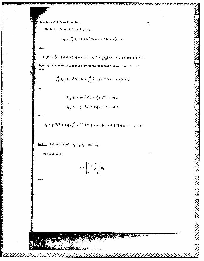
Similarly, from (2.6) and (2.8).
where
K() .- ,V7[sinh 71(1-1l+sin 7~(i-j)) + 62 (-)cs(-)]2q ~~*~ 2 [cosh 71( co
ieeting this same integration by parts procedure twice more for f,
0 2 71eI'2~ed f= 5 27 (f)iV'(()df 2f,
1 -1 71 2 -71fK27 (f) =In~ e (1+ik 2 7j)e *0(1)
K f m113 2 -,,It
*~ uget
h I -le (1+ik'nf e"'q(iV(( ).g(Q)dt O(Ilf"Ill*Ilgil). (2.16) I"2 -4'" e 1)S
WrdSWe Estimation of A1 .A 2,A 3 and A4.
We first write
o 2J
where
*R W. ,

78 Chen, et al.
(71,el 1- l 1--k ) ( 1-k 1e i
2)1 --7. -n~ -1 -ik. e I iU
So
A2 0
A3 Ml ,-2hA I -2h
Further, write
M1 (det M )--21 122
Mi~i I'31 '"32
From the evaluation of cofactors.
~12 - (1-i)[((-ik e'77 - i(1+k )e'77 + (1+)(Iinkf)e71]
Z()1 ' (1ik)[(k2e" -2 (1k1e7 +111(1+k )- )
2 (ii(-222 2-221 -7
2217i1+-I ) ( 1+k k2 )+2k 17 l
The term in braces above satisfies .'
I ( H I Bracket 21 -I Bracket 11
~2(1+k 2 2k 2 ), as 41-
1 2'
J .4-

-B .:I~'ernoulli Beam Equation 79
If > 2 for i, sufficiently large,
lie
IZ(t) > 2, Z( ) 72
) (217)
D1 a det M, (1-lk2)e .u I + (l+iik2)e77 1 + 0(72)
" Z(')e 7 O( 2), therefore
= (e 7(7)Je- + O(e' ) (2.18)
n d by (2 .17 ). "
D- 0(7i le1). (2.19)
(2 15). (2.16) and (2.19),
A Di (.1 1h1+"12 h2 )44
(0-1) . I 71
Z , en f ( g df +0( -
8 PIIP 2 are 0(71). Continuing from the above:
4T e 7)fo' ~-
+
+ O~e ' [ll~ll~lgll])(by (2.17), (2.18))"'
= 1 - '[{P ~()d + (77e-I e11Cf"(f)*g(e)]d( ;j
k
"
P
1%
F IPWVp.
Opp V~ - *-.
,.,.

80 Chen, et al.
0fZe i,(),(} ( [lfiil~ileII]).
Thus
A112 -4q 'So e[" if' Qlg( jd 0 e [JIf"11I'iglI]) (2.20)
As for A2 . we have
A2712
Di (#21hl P22h2) (2.21) *J.
where
By (2.15). (2.16), (2.22) and (2.23). the domiiiant terms In 1,2 1hl and
"22 h2 are O(77e 2 71). But their coefficients in u2l h, + P22 h2 are such
that they cancel out. We get
2 -1A2n2 D1 O(ie"[llfIllIlgll]) = O("f' lgll) (2.24)
Similarly, we can show that 2,I).
471 2 = O(lf " Ilgll) (2.26)
Final Steo Estimation of )1l1w"1 AI.
By (2.14) and (2.20), we have "
.- %
S
P*
77-. '-1A -O0

Euler-Bernoulli Beam Equation 81
w"(x) -, w"(x) w(x)
= 1. -eX e' /(ilfl(fl~gl(]de2 Oclf- [lf'lllgU]) 1V e o
* ,21i At 2 1Ix A 1 ~ 2e -1ix *2 e ?IX- A l?2 ; lix + A 2 (..,2-') x A 3 ( ./ 2 - x A4 . (_ 2 1 , x
= (00-1 tllf"jl-!lgj]) + e 7X
O('0e7 enflf"I-jgli])
+ (-A 2,2e i .x 3 712e- x - A4'12e- ilX),
In the first parenthesized term, the X2-norm of e'I
x is of order of
magnitude
(ellx)2dx]l/
2 1 [q(e2711/2 3 Ohq-1/2el)
0Nhence
I first parenthesized terml 2dx]1/ 2 . O(if"ll+lgl).0
The second parenthesized term also satisfies the above bound, because of
(2.24), (2.25), and (2.26).
Hence
IIw"I1 S C(llf"ll+llgll) - O(llf"ll. llgll), for q large. (2.27) %
For v, by (2.4) we have
Ilvil S I I+wI If -l. (2.28) .
We want to show that
1 12 11W1 2 < C(lIl Il2 ll 2*llfll 2.llg l2). (2.291
for some constannt C > 0 independent of X.
Consider (2.2.1). with =4 I and X - in 2. and use k2, k
2 for
1 2k and ;2. Multiply (2.2.1) by w(x) and integrate by parts twice.
We get %
%.
4 4

--WWW+WV-WWWW LWVk"WPF TWA82 Chen, et al. I
w"( w),(i).-w"( )q'(t ) + 11w"112 - 41 2 =
=-<f,',w>+<"w>.
From (2.2.3) and (2.2.4), we get
=-<f,Nw>~<g,w>.
Hence
1 4 lw1l2 = Re(llw"l12+<f,Xw>+.<g,w>+k2f(1)w(1) k 2 f (I)w (1))
_< Ilw"J 2 + 4JL, Jw2 +211fh 2+ 1 e2 1 +JjwlJ2 2f+iiw..12],
where we have applied the Poincare inequality and the trace theorem:
iflI)l2 . if,(1)1 2 <_ (:llf,,ll2
lw(1)l 2 + Iw' (1)l 2 5 CIw"lj 2 .
Therefore (2.29) follows for 17 sufficiently large.
By (2.27) and (2.29), we have
Ilvll <- C(llf"ll-llfll+llw"ll+!lgll) (2.30)
C Ilfll < ll f llas
and (2.27) holds.Combining (2.27) and (2.30). we have, proved (2.5) for J1"
sufficiently large. X - iw. w E R. So Lemma 3 has been proved. 0
THEOREM 4. Let k2 0 and k2 > 0 in (1.I). Then the uniform
exponential decay of energy (1.2) holds.
%,
i -' " - " .... .. . "' '. ++P 5 , r: +"'+
a-
Da"-
* S.• i

83 Euler-Bernoulli Beam Equation
Proof: In order to apply Theorem 1. we need to verify that assumptions
(1.6). (1.7) and (1.8) are satisf(ed.
We note that (1.6) Is satisfied, because A is dissipative and
ffexp(tA)II _5 1.
The verification of (1.7) and (1.8) is accomplished if we can
verify merely (1.7):
(AI-A)- 1
exists for all A = iw, w 6 R. (2.31)
because by (2.31) and Lemma 3.
IlwXll + IlvN JI S C'(llf"ll+1lglj), VX = Ic. w C R,
where
C' - max(C.C"). C as in (2.27) and (2.30)
C" a max I(lXl-A)-II, for some B2 sufficiently large, NI -ji5821, f e 2
To show (2.31). we assume the contrary that o(A) n (ticj e P) .By Lemma 2. o(A) consists solely of isolated nonzero eigenvalues.
Without loss of generality, let
X e o(A). X0 112 0 E R, 70 0e 0.
Then
(Xo'-A) v0 0
has a nontrivial solution (wov 0 ) C D(A). Explicitly. (wo,V0 )
satisfies
2er2 '- #- v: -. - . . :: g : ¢ ¢e; J - : : "' ,.,' ,''e",.. .; .-..;, -.,x:, ,I,.

fl ., W WVV UW fW ~WMUMUM W V WW WVV i V--
84 Chen, et al.
17 2WO -o VO 0 on (0.1]1
( ) 2w ij v . 0 on [0,1]
WO(O) -0
W6 0 (1
w-d(I) k2 vb(l) _ 0
Letting
w(x,t) =e 0t WOW.)
04we easily check that w satisfies01
w ~ 0.
Also, the energy
0
d f Ref w~c(x.t) xtx.tu1w]xt~ct]~
--2(k~Iwt(1.t)I 2 .k~lj w(I.t)j2~
Because k2> 0 and k2 >0. we deduce 121
2 , 'WI~ ?1
OIW6(1)' 0

Euler-Bernoulli Beam Equation 85 52.%t Iwxxx(1.t)I - Ih(l)I - 0. it ki 0: %.P
x (1tL) - lj-6(1) - 0. Iwt(1.t)I ,2lwo(1)l 0, if k2
> 0.
Thus wo(x) is a solution to the boundary value problem e
(4 ) - ' 0 0 on [,01]0oO =1 0 0
w(0) - 0
(2.32)
wb(l) . 0
w'(1) - 0 .
w (1) - 0
Write V
W(X) A 0 1cos '/0(x0 -l) A0 2 sln i 0(xl)+A0 3 cosh 70 (x-l)}A 04sinh 170 (x-1)
Then the five boundary conditions in (2.32) require that %
5.'.,
cos -sin o cosh " sinh no Ao1 .sin n0 cos no -sinh no cosh no A 2 %
0 1 0 1 /A03 -0 (2.33)
-1 0 1 0 A04 j
0 -1 0 1
has a nontrivial solution (A01 ,A0 2.A 03.A 0 4 ). llowever, it is easy to
check that the matrix In (2.33) has rank 4 for any no e R, no 0. a e.
contradiction.
Therefore the proof of Theorem 4 is complete. 0
1%
3. ASYMPTOTIC ESTIMATION OF EI(;ENFREII1ENCI -S
From the graphs in [2]. one notices that at low freuuencirs
eigenvalues of the damped operator A seem to exhibit a
structural dampin=" [31 pattern. Does the structural damping pattern
II
-N,
le%
b.
Ram .,

86 Chen, et aI.
continue into high frequencies, or is it only a low frequency phenomenon,
for beams with boundary dissipation? To answer this one must examine the
asymptotics of etgeafrequencles.
The work of asymptotic analysis was first done by P. Rideau in histhesis [8] (cf. the acknowledgement at the end of the paper). Unaware
of his results, we had carried out the analysis independently. We feelthat It is of significant interest to include the work here as it will
make the study in this paper more complete, and only a minor effort is
required.
Let (M(x).*W(x)) be an etgenfunction of A belonging to theelgenvalue aX(;O). Then by (2.2). setting f(x)= g(x) a 0 and wx - 0.
we see that 0 satisfies
04 0l4l(x)._ X2(x) = 0'€(0) - ' (0) - 0€ (1) - ),;1 (1) - 0 (3.1)
1(= o "1' .p
To simplify notations, we consider the following elgenvalue problem.
01 4)(x + 2lx) 6 ,
0(0) = 0 -
-10 A0( (302)
2.
€ *(0 k0_ (3.) ,* 0"
Noting that the following correspondence
A
a2- In (3.1) k2 in (3 2) (3.3)
2 T1
Is in effect.
The boundary value problem (3.1) has a nontrivi;tl solution if andonly If
P1%
j%
% 'S
* C-,
. - • - =, =p - .r • .= , , • . = .- . ,,, , - " -. , " ".%, % ". ",%, ".% % %j, %
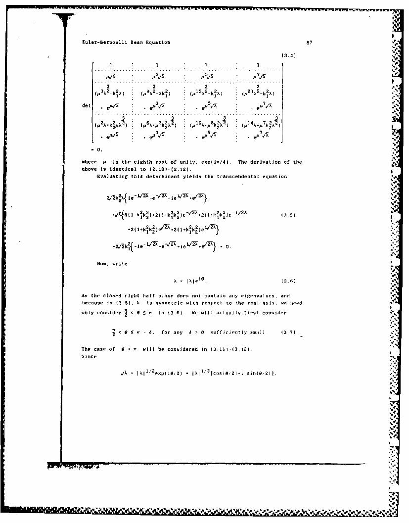
Euler-Bernoulli Beam Equation 87
(3.4)
............ ................: ................ .............
pM ,,Kp%- p7/3 . 3 . 3 . 3
............ ................ ................ .......3 3 3 3de ePV ep3
" .X .P 1/X • p . e#J3.'
2 3~ 3 13 52 41A 2 Xk 2 X2) OA6xA ~ k2 .\") 10) Xjp 5k 2 X2 1 Aj +pA k2X-2
-0.
where ju Is the eighth root of unity, exp(iit/4). The derivation of the
above is identical to (2.10)-.(2.12).
Evaluating this determinant yields the transcendental equation
Zj2 fI e - ei./ , -2) -X
-e e e' } %
2 28k2 ki'2" -V2"Xk iek 2 /2"X.e 2 2 O./2
Now, write _
1= 2Xleie e (3.6)
As the closePd right half plalne doP.s nnt conttin i=rcy eIigonvajues. and "
because in~ (3.5). )X is .symmntric with reslpeCt to the real axis, we need
onl cosidr < 0 _< a in (3 6). We will atualy first consider '
S< 0 <_w - 6. for any 6 > 0 su[fficintly smal] (3 7) '
The case of 0 4 a will be considered irn (3.11)-(3.12}.
+1= I)kkt2exp(/2) i/2cos(O/2).I sln(G.,2)J.
C',
1 2 1
U~ ~ ~~2 I, 2xU~-p4 ,. a*=SC-S

88 Chen, et al.
we see that
e2- = e-2-TCOS(/
2)e-L/2- sin(e/2)
e4.= 4'
e VTl~(~2 e i,2..csG2
are ( -7 T' ^T) for some 7 > 0. Thus, from (3.5)
a/-,(lk2 e - 4/2 +2(+k~k2)3 12/-k0]
eV2X[2/./k 2 X2J(.l+k 2 2.)+ 2] O(jI) exp(-,yT.T)).
which implies
e/2T T[-sinle/2)cosle/2)] - -e-L./2'T[cos(e,12)+sin(G/2)]
t~ 2 122- -2,22X+2( 1 k2 j~)./k
But (assuming k2 > 0) the term in braces equals W,
2 2
J(1,1) (l+klk 2 ) e-1 G/2 + O(pI)I.
Thus we seek X's satisfying ',
e -',/T [-sin(e /2) cos(e /2)] (381
%'
We observe immediately that 0 - w/2 as IX) - o, since the LHS of
this equation would decrease to zero otherwise. Furthermnore. theequality can be satisfied (up to higher order terms) only whon the firstterm on the RHS is a kositive real number. Thus
'6.'p
A._
6|
-?%"k -11

Euler-Bernoulli Beam Equation 89
e"V
2 ]X'T ~e
o%(e /2
)*s tn (
0/2
)] .Z e-"/4T- 2.
wp
or
(2n - ~ 2
IXI [- , n is a large positive integer. (3.9)
The above gap of Oln 2 1 for elgenvalues is common for Euler-Bernoulllbeams with energy conserving boundary conditions. Now we see thatEuler-Bernoulli beams with boundary energy dissipation also have this
property.One checks that when the RHS of (3.8) is real. its modulus is
22 .(lk k2 )[cos(e/2)lsln(e/2)] -).i " [ '[T"O(iXl %
This in turn Implies that tile exponent on the LIIS of (3.8) must satisfy
- _in()+cos)- (kk) cs(]zsin )
if we now write 0 = c . t > 0. and expand to lowest order in r.
we have
12
-l 22 2 /Now suppose X - , l'.. Then G tan -(7/() and IAI (f 2? ,T.
or
Exadn ta'4bu q(=owehv
~~S V-A , -.V % ."% A %
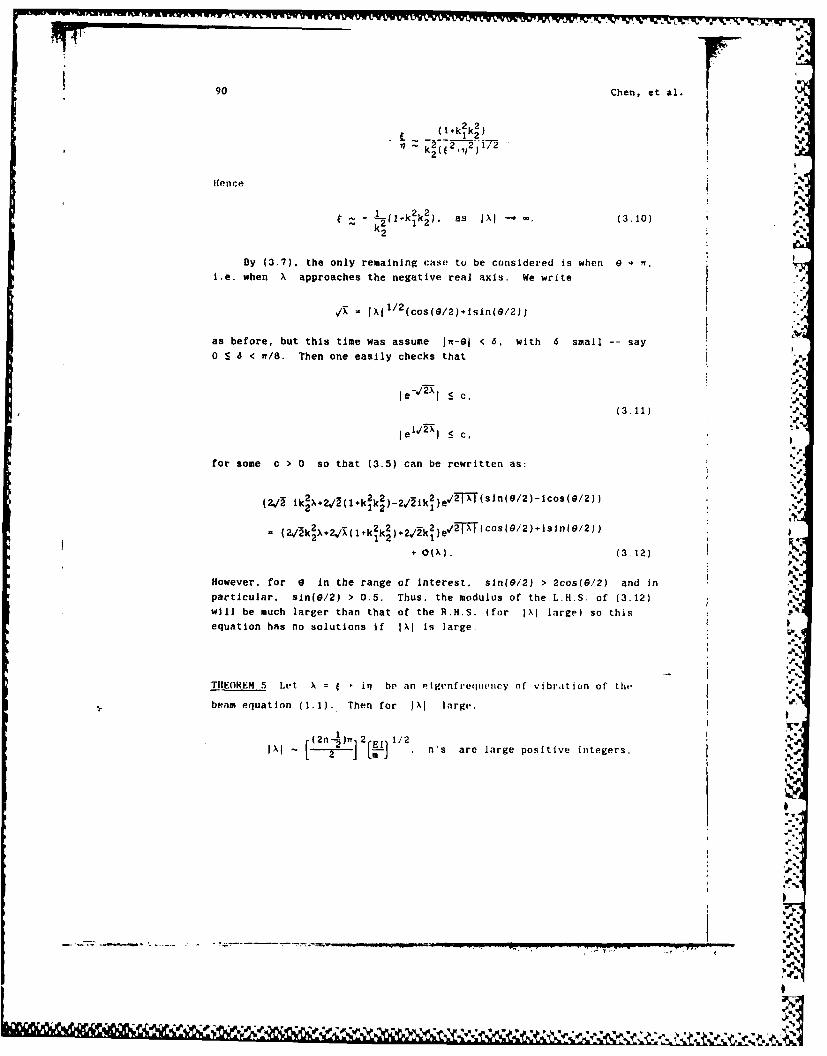
90 Chen, et al.
;-" llence )1~ 22
By (3.7), the only remaining caseI to be cnnsidered is when e - .. -
i.e. when X approaches the negative real axis. We write",
.. f 12
1/ [[/2 (cos(G/2)+isin(G/2))
as before, but this time was assume ja-el 8 , with 6 small -- say
0 <. 8 < /8. Then one easily checks that I
1 , ~(3.11) '.
for some c > 0 so that (3.5) can be rewritten as: ,
Ifenre %
(=J ik-4 1k2-Ji2 e- T (csn (9/2) -i csn( o/2) ) .'
* Ol2). (3.12)
However, for e in the range of interest. sin(G/2) >2cos(9/2) and in q..__
particular, sin(G/2) > 0.5. Thus, the modulus of' the L.H.S. of (3.12) , :
will be much larger than that of' the RH.S. (for ]×( large) so this-:equation has no solutions if I a Is large. c
TlIE.Iwh 5 Let X = apr iah he an e algenfreqlu~cy of vibr ,tion of th.beam equation .1). Then for eX large. that
t-* ~ le ns ar ge pos tve
I
(3.11)
'
'S'%
(2/ ik -X2,I .r---- 2 -rT7;l(02-co(/2 1 k2)-2r~ik1 )e
(2 h2 \2,/-~l~2 k )+,( 2 )v,27X (os(/2)+s1./2)2 1 2 1
+ O(A)(3.12
Howver fo 0 In the rang of Inteest si'S)> cs )adi

wInw N-
Euler-Bernoulli Beam Equation 91
2 as I'l (3.13)
Proof: Just use (2.3), (3.3), (3.9) and (3.10).
By (3.13), the eigenvalues will be distributed nearly parallel to
the imaginary axis at high frequencies. Therefore there is no"structural
damping" when the frequencies are high. This has also been confirmed
numerically in Rideau's thesis [8].
We note that when k = 0 and k > 0, asymptotic limits can be
obtained in the similar way.
4. DESIGN OF PASSIVE DAMPING MECHANISMS'U
The following is a (more or less exhaustive) list of combinations
of dissipative boundary conditions for an Euler-Bernoulli beam:
-Elyx(1,t) = 0-k2 }
-EIYxx(1,t) = I (4.2)
-Ely xxx (ZI )=- ytt) 0 (4.2) .
y(1,t) = 0 1-EIyxx(1.t) k2yx t(1,t) k
2 > O (4.3)
-E lyY(,t) = k2xtl t ) c2Yt(1.t) > 2
where in (4.5). c1 and c2 are real constants satisfying
o.;"4
I 4.xd ..
(c I- 2I.. 2a -, 0 V 6 46
% %4

.. w ww uw wu NWW WWWUWV wvw~d ' WVW'h WUWV VW WW w Ws W'W v'w V% Vww 'WjVMjVr'jVWW
92 Chen, et al.
Note that the boundary conditions (1.1.4) and (1.1.5) correspond to
c, . c2 - 0 in (4.5). Obviously, (4.6) Is satisfied In this case.
We want to show that all stabilization schemes (4.1)-(4.5) canj be
realized in practice, at least by designing passive dampers.
As (4.5) seems to represent the most complicated case among i(4.1)-(4.5). we treat It here, at least for certain special values of c
and c2 (cf. (4.7) later). The other cases can be studied similarly.
The following damper arrangement gives a design which effects the Vcoupling of shear (resp. bending moment) with velocity and angular
velocity:
hi
h/2
a) Inclined Damper
Vs [Ly(lt) s e h ] co Vs Cos
Cv s
~~of Damper -:
-%Shear(l,t) =-c. d' sin 9
Moment(l,t) c d v ] Cd v h/2
Fiue2 Damper arrangemLL.t for ( ,...
ILI%
C%
dv5, .
- "; • " %) I = ,' %%,%' %, % .".-.% " %-,%." -,%C v .j n 9
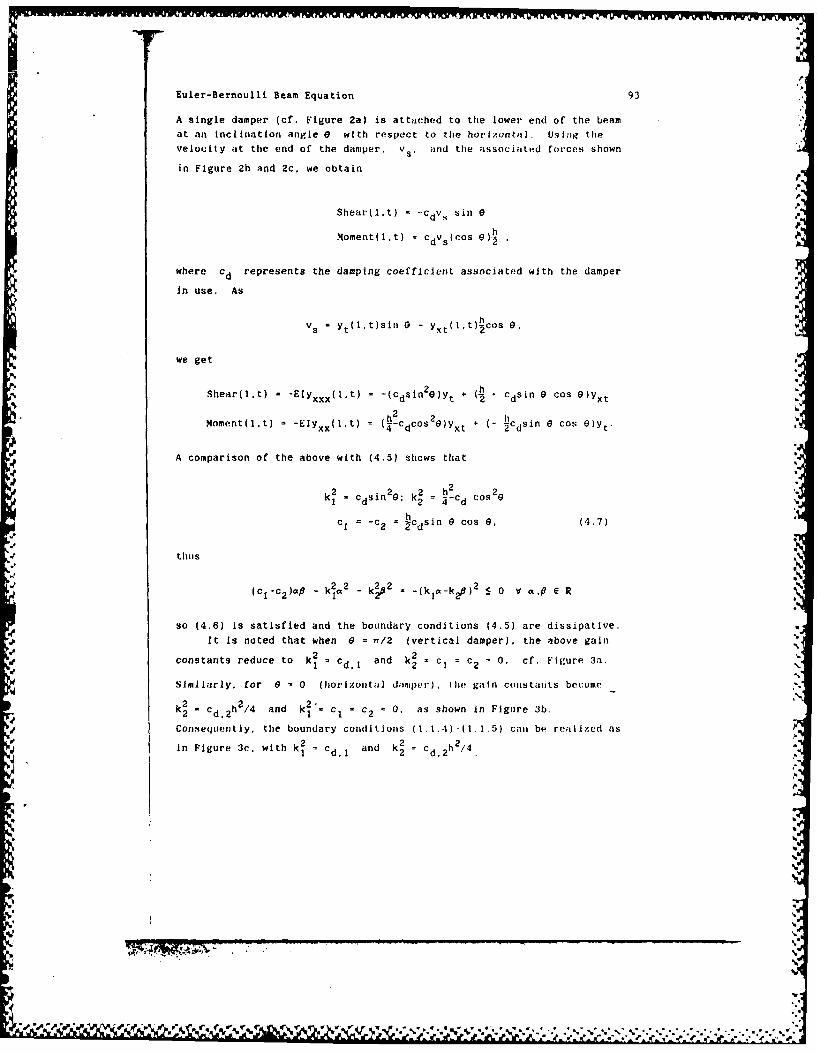
Euler-Bernoulli Beam Equation 93
A single damper (cf. Figure 2a) is attached to the lower end of the beam
at an inclination angle 0 with respect to the hoz1'7ontn. Using thevelocity at the end of the damper, v s , Mnd the associuted forces shown
in Figure 2b and 2c, we obtain
A
Shear(Jt) = -CdVS sin 0
Moment(1,t) = CdVs(cos h ,
where cd represents the damping coefficient associated with the damper
in use. As
v s = Yt(,t)sill 0 - Yxt (It)hcos 0.
we get
Shear(lt) = -ElY xxx(lt) = -(cdsin2e)yt ( h2 cdsin 0 cos O)Yxt
h hMoment(l.t) -Elyxx(t) = (h-cdcos e)yxt * - cdsin 0 cos O)y,.
A comparison of the above with (4.5) shows that
2 2 2 Cos 2
k2 = CdSi n2 ; 2 i = hd
c 1 = -c 2 = PCdsin 0 cos 0, (4.7)
thus
Ik c kjO - -(kja-k) S 0 a
so (4.6) is satisfied and the boundary conditions (4.5) are dissipative.
It is noted that when e = r/2 (vertical damper), the above gain
constants reduce to R =Cd and k2 . c = c 2 = 0. cf. Figure 3a.d %"
Similarly. for 0 = 0 (ho'lzonta l damper ), the gain constalts become
k2 = 2 /4 = c 2 0 0, as shown in Figure 3b.
Consequently, the boundary conditions (1.1)-(1.1.5) can be realized as
in Figure 3c. with k 2 Cd. 1 and k = Cdh2/4.
-.1 ,.. .. , ,. . .

94 Chen, et al.
h/2
x=1
h/2
cd (It Cd y (l,t)h/'2
Shear(1,t) -c Cd Yt (1,t) Moment(l,t) c Cd yxt(l,t) h 2/4
a) Vertical Damper b) Horizontal Damper
Cd
4HC d
X-1
c) Shear(l,t) =-cdytC1.'t) -
Moment(1,t) -= Cy (l't) h/
Figure 3 Damper arrangement for (4.1), (4.2) and (1.1.4)+(1.1.5)

PWI w PIP% An gt WI W.PI "n~rlwljwvM
Euler-Bernoulli Beam Equation 95
£O2
Shear(l,t) - C dYt (1,t)
Slope(l,t) -Y~ (1,t) -0
Figure Damper arrangement for (4.3) Sp
c'
%.
Y(I-t)
Momet~l~) cY, t(l~t h /
Figue Daper rranemen for(4.4
Cd --'p..
r.

96 Chen, Krantz, Ma, and Wayne
The otner boundary conditions (4.1)-(4.4) can be realiszed and
designed, respectively, as in Figures 3a, 3h, 4 and 3.
Tire method of estimation which we have developed in this paper andHuang's theorem (Thm. 1) can be applied to study exponential stability
for all of these boundary stabilization schemes.
ACKNOWLEDGEMENT We wish to thank M.C. Delfour for pointing out the
thesis of P. Rideau [8] to us. where Hideau has already carried out the
work of asymptotic analysis of elgenfrequencies. The priority should go
to him. Recently, we have also found that D.L. Russell [9j and his Ph.D.
student S. Hansen [5] have independently obtained similar asymptotic
results.
REFERENCES
[1] G. Chen, Energy decay estimates and exact boundary valuecontrolabillty for the wave equation in a bounded domain. J. MathPures AppI. 58(1979), pp. 249-273.
(2] G. Chen, M.C. Delfour. A.M. Krall and G. Payre, Modeling.stabilization and control of serially connected beams. SlAM J. Cont.Opt., to appear.
[3] G. Chen and D.L. Russell, A mathematical mode.l for linear elastj(systems with structural damping, Quart. Appl. Math. 39(1981-82).pp. 433-454.
[4) F.L. Huang, Characteristic conditions for exponential stability of* linear dynamical systems in Hilbert spaces. Ann. Diff. Eqs. I(1),
1985. pp. 43-53.
(5] S. Hansen, Private communications.
(63 T. Kato. Perturbation Theory for Linear Operators, Springer-Verlag.New York, 1966.
[7] J. Lagnese, Decay of solutions of wave equations in a bounded rregion with boundary dissipation. J. Diff. Eq. 50(1983).pp. 163-182 S.
(8J P. Rideau, Controle d'un assemblage de poutres flexibles pat- des
capteurs -act ionreuls ponctuels; etude du spectre do systf.m('. Thes,L'Ecole Nationale S'iperleure des Mines de Paris, Sophia-Antipolis.France, November, 1985. A
L1 9] D.,. Russell, On mathematical models for the Plastic heam withC frequency lroportionl dampiIg., to appeal.
.4
L"71
-oo , .,..-
SI . , ,,
S - - . .. ,- ' *. . : 2
__ _ __ _ _ __ _ _ __ _ _it
- ~ %~%9 ~ \'%4( Q~'; . ,.'j~ P'." ' *41. ~%'%%~* ./.,,''\' i.",' ',.V 1%%C.

"S
.3
,, ,
_'__
..............TF'i,.