- 51 - TODATA-

SAMPLE PAGE FROM TOD DATA DESCRIPTOR DICTIONARY

Y x

5

: CI ” m w x

. z x

vi

Y-2 VQ WO

zz

a w l-4

In ul N 0.

Wr: ww Ct”

m ua

CL

r-l co m LL

: t-1 D.

ACME Note

- 52 -

The TOD Databank Description Language

TODDDL-1 Steve Weyl.

April 3, lg:,

A. The TOD Schema and DDL:

A TOD databank is constructed and accessed according to a carefully defined databank description called a schema. The schema is specified by a set of 'high level" language statements which are stored on a textfile, much like a PL/ACKE program. These statements are translated into an internal form by the schema translation program, TD_TF?A (ACME Note TDPT).

The high level schema language will henceforth be referred to as the databank description Language, DDL. The syntax of DDL resembles PL/ACIGE syntax, except that it only provides for declarations. DDL is designed to require accuracy and completeness of definition, since these are essential for effective databank operation.

The schema serves two important functions: First, its DDL representation gives an explicit documentation of the content, unit of measurement, reference name, and type of each data item; and it indicates the data initialization, range checking, encoding, and retrieval file maintenance which must be performed. Second, the internal form of the schema provides generalized TOD programs with information about the structure of a specific user's databank (see example in ACM3 Note TODD, Part III, Section A.2.d.i.).

The necessary information for writing a DDL schema can be accumulated and proofed on a convenient printed form, copies of which may be obtained at the ACME office.

B. Basic Semantics of DDL:

A "single piece" of information is stored in a data item or just item. The in- -- formation stored in an item is referred to as the value of that item.

The items of a databank can be partitioned into two general categories. Items in the first category are recorded only once and they store demographic information or background information associated with a patient. Items in the second category store the numeric values of several time-dependent parameters recorded for each patient-visit. A 'visit" corresponds to a physician interview, or any other point in time at which information about a patient is logged.

DDL repre=- uLnts the two categories of data items as formal arrays. Each formal array element corresponds to a single data item, so that an array of elements is a list of related items. The category of demographic items is represented by the HEADER formal array. The category of time-dependent items is represented by the PARAMETER formal array.

The size of each formal array, and thus the size of each category of items, is established with a declaration statement. Then each formal array element may be assigned a 5-tuple of attributes. These attributes describe the data item asso- ciated with a formal array element. The attributes define content, a measurement wit, rxux, hti? t,l~z. x6 ret7:e-;al t:;:e frr 2~ item. T‘na c: -i ~-es forms1 zrray _A/-.. ahGL* eie;,,c;lts hi'e p;~~e-~iulu~rj e;;pcu,i,ing Liie irl~Ti)tiUCLiOIl 01' hew &La itema inLO LrAl databank.

- 53 -

TODDDL-1

The INITIAL statement allows a user to define the initial (i.e. default) value of each item prior to data entry. Careful assignment of default values can re- sult in major savings of secretarialand processing time. Also, by reducing the amount of data which must be entered per patient-visit, the data entry error rate will be lowered.

54 -

.

n aJ

- 55 -

D. Detailed Semantics for DDL Statements :

TODDDL-1

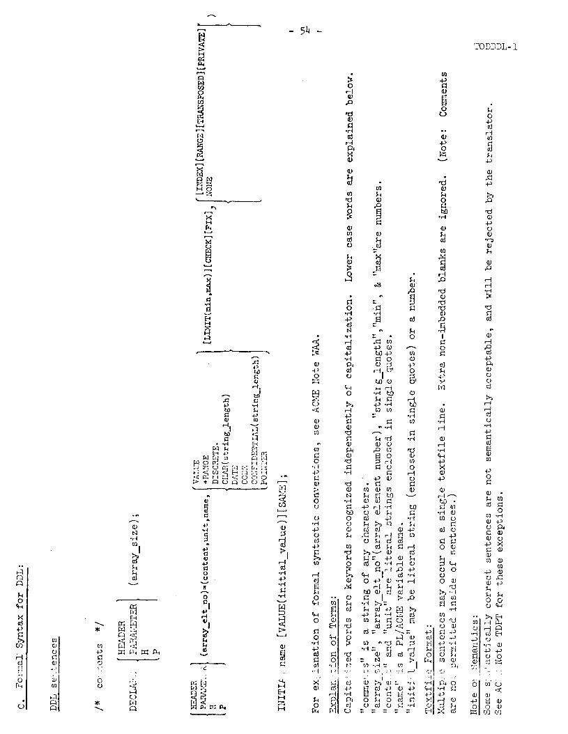
Comments, enclosed in the PL-conventional "/*I' and "*/" are ignored by the schema translator and serve only as documentation.

A declaration statement specifies the number of elements in each formal array. Before data items can be assigned attributes, their associated formal arrays must be declared of adequate size. II I, H and "P" are recognized abbreviations for "HEADER" and "PARAMETER".

The formal gssigrment statement defines for formal array elements the attributes of their associated data items. There are five attributes which must all be specified. We will consider each separately.

The first attribute of a data item is a character string of length 540 describing the content of that data item. For example, if a HEADER item stores the address of the referring physician for each patient,its content might be described as 'ADDRESS PHYSICIAK' . The content attribute is included in documentation purposes. It may eventually be used composition of Time Oriented Record forms.

The second attribute of a data item is a character

OF REFERRIIiG the schema for for computer

string of length 510 describing a standard u of measurement. For ex2r@e, if a

PARAMETER item stores the white blood cell count for each patient- visit, its u?jts night be describe? as 'x.zXO'. Aunit muat always be specified and a null response will not be accepted. For the HEADER item suggested in the first example, itsunit would have to be specified as 'address' or 'none'. The reason for always requiring units is to assure that databank planners fully specify the mesning of each data value, SO that d2ta can be shared.

The third attribute of a data item is a (short) name by which the data item may be uniquely identified. This name must be a valid PL/ACXlE variable name. Names will always be reccgnized irrespective of capitalization. In the second example above, "WBC" might name "white blood cell count".

Names are an important symbolic attribute of data items, and the use of standard names will greatly simplify communication of infor- mation between two data banks and zierging of data banks. To assist in the standardization of data item names, a sorted list of names and the attributes of their associated data items will be maintained by the TOD manager.

Public databank procedures will make use of certain standard names for automatic update of data values. For example, the data item named "age" will automatically have the current age of a patient stored in it (as computed from the "date" for this visit and the "birttdat" i'ern for :,?-.is p,a",i?nt). These standard items are de- ;'lEeci iri section L.

- 56 - TODDDL-1

In the INITIAL statement, HEADER or PARAMETER elements are identified by their names.

Names will be used in tabular output programs for column headings.

The fourth attribute of a data item specifies the data type of information stored in this item. The following types are available:

1)

2)

3)

4)

5)

6)

7)

8)

VALUE data items can meaningfully assume continuous numeric values with six significant figures. They are stored as ACPIE single precision floating point numbers. VALUE data items are assumed by analysis programs to be measured on an interval scale.

+RANGE data items can assume the values 0, 1, 2, 3, 4 (of the "+RANGE scale"), which is treated by analysis programs as an ordinal scale.

DISCRETE data items can only meaningfully assume discrete numeric values. AnalysLs programs consider them to be measured on a nominal scale.

CHAR(string_length) specifies that a data item has as its value a string of variable length 5 "string_length".

DATE data items store dates in an internal form. Dates are entered in a standard format, DDMONYY. DD=two digits specifying the day, MON=first three letters of the month (irrespective of capitalization), and YY=last two digits of the year. There are no spaces. The standard form is auto- matically encoded into an internal "arithmetic date" for storage and nu- merical manipulation. Storeddates areconvertedbackto externalformby TOD retrieval modules.

CODE data items are stored as numeric values related by encoding-decoding procedures to a more legible representation. For example, the item "sex" might be coded as 0, 1 for F, M.

CONFIDENTIAL data items are encoded and decoded by private procedures pro- viding keyword-protected scrambling. Only READER information can be con- fidential.

POINTER data items store pointers to information contained in an auxiliary data file, defined for a specific TOD databank. What gets pointed to by a POINTER items is determined when an individual TOD databank is defined. As an example, a READER element of type POINTER might point to the first of a group of textfile lines comprising a reference letter for each patient.

There are three data type qualifiers. At data entry time an item for which LIMIT(min,max) is specified will have its value checked. If the entered value falls outside of the specified limits, an error message will be given.

At data entry time an item for which CHECK is specified will have its value checked fcr validity 1:~ the user-provided encoding-decoding data check proced.Jr?s / ,. . . [Se< iiL:- -I_ ii- .-

L-~a~.j. iC;..,.5 C’S,’ e*ei*iL‘Zl Tir. 15 ~~e~~fie~ ;;ill PA--ye

their values checked by a big data checking program run incrementally against the databank asynchronously with data entry.

- 57 - TODDDL-1

The fifth attribute of a data itcn specifies the retrieval m for information stored in this item. Retrieval files will be maintained by a public UPDATE program facilitating the retrieval of data items in accordance with their retrieval types. Like the other attributes, retrieval type cannot be omitted from the formal assignment statemen-';. Any subset of the types INDEX, RAmGE, TRANSPOSED, or PRIVATE may be given for retrieval type, or else the user must specify the type NONE. PRIVATE indicates that a user maintains private files to ex- pedite retrieval for this parameter.

Leaving several formal array elements undssigned with attributes greatly decreases the cost of adding new data items at databank re- compilation time, and is highly recommended. Assignment of previously unassigned formal array elements is a relatively inexpensive way of expanding a data bank, whereas redeclaration of formal arrays leads to costly reformatting of the entire databank.

The INIT=L statement causes the data items corresponding to a named formal array element to be set to an initial value given as "initial- value" prior to data entry, checking and encoding. If "SAIJE" is specified for a HEADER element, it has no effect. If "SAKE" is speci- fied for a PAFWiETER element, then it has the following effect: On the first visit for each patient, this parameter element is set to UNDEFII!ED, or to its initial value if VALUE (initial-value) was indicated. Then for each successive visit thic item's _ w11.13.~ j.s iyeitiy--liZCd to if-q - -- value on the previous visit for this patient. If no initialization is specified, numeric values are automatically set to "ULIDZFIIZ3D" = -0.0 and string values are set to null as a default.

Formal array elements must be assigned attributes before they can be assigned initial values.

Declarations of formal arrays must precede use of formal array elements, and an assignment of attributes to a formal array element must precede its initialization. If several assigrJilents or initializations are specified for one formal array element, only the last will be effective.

E. e- Required Items:

The folloi;ini; three iZY.DZR and two ?XXJETl;P ele,-.cnt assigments ;1uz+ be included i.. every d.c.f,:;ank definition if a user uis3es to take aCvx.L,a<t of public data entry and retrieval programs. The assignments are written in DDL with explanatory comments. Data type qualifiers and retrieval types other than NONE are acceptable throughout.

- 58 -

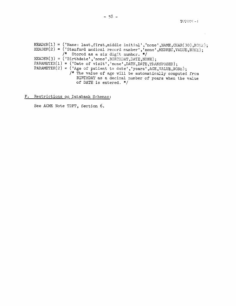
HEADER(l) = ('Name: HEADER(2)

last,first,middle initial','none',NAME,CIIAR(30),NONE); = ('Stanford medical record number', 'none',MEDREC,VALUE,NOEE);

/* Stored as a six digit number. */ HEADER(3) = ('Birthdate','none',BIRTHDAT,DATE,NONE); PARAMETER(l) = PARAMETER(2) =

('Date of visit', 'none',DATE,DATE,TRANSPOSED); ('Age of patient to date','years',AGE,VALUE,NONE); /* The value of age will be automatically computed from

BIRTHDAT as a decimal number of years when the value of DATE is entered. */

F. Restrictions on Databank Schemas:

See ACME Note TDPT, Section 6.

- 59 - TODDDI.,-1

logy Databank (AC 4 I

*. I

. . LU CU LU -. -r 7 - r. - ~_, .., .>

,-

c 0

!d

LU Tj 1’

.

.:: r?

G. Example of a DDL E of the I ,

*. . .

-A

i i

Dist: Staff/TOD/All

- E@ -

Core Research 8c Development (Llont inut2tlj

Anal-,yz i 111’ ‘1’011 Operat; i.orKI (:ost.::

!Carly dur irlg .i,he ‘i’OL! prc~~jrct, Ike f’c~l~rlr! l.k1:11, phy:; i c i ans (1 i d rJc>l, have tile l.ool s avai~lable Lo get an adequate pic:l,~~re of the operational costs of a databank. They knew their total costs and what they did, but the task of allocating costs to individual transactions had become complex. An attempt was made during the pro5ect to set up a cost analysis frame- work to aid the researcher in determining where his computer dollar went. ACME Note TODCST outlines a study underway; ACME Note TODPDA outlines the method of trapping basic cost and transaction data for the TOD system. Note TODCST follows.

ACME Note

- 61 -

Analyzing the Costs of Running a TOD Databank

TODCST-1 Frank German0

March 22, 1373

This note outlines a study to analyze the costs of running a TOD databank. Com- ponents of costs and procedures to compare them are identified, both for compar- isons of cost components within individual databanks and among several databanks.

The outline described in this note will be used to compare TOD costs in Immunology and Oncology, two operational TOD databanks. In the future, as the number of TOD databanks grows, the benefits of cross-databank cost comparison, as outlined here, will increase. In any event, cost comparisons among components of a single data- bank are always useful.

Raw Data Sources: The raw data for analyzing costs of a TOD databank can come from several sources:

(1) ACME end-of-billing period accounting detail which shows LOWN- LOGOFF pageminute charges by account.

(2) TOD program TD-CSTCK output. (3) Independent logs kept by TOD users.

Each source yields information on some aspects of the cost picture. All have cer- tain biases which should be understood.

ACME End-of-Billing Period Accounting Data: The ACME end-of-billing period accounting data is the most critical because the monthly bill is developed from it. This is the number we are trying to analyze and justify. At present, an ACME user only gets a monthly bill showing totals for disk blocks, pageminutes, and terminal connect charges for the month. The logon-logoff detail is only provided on special request.

Since this detail is only identified by date, time, terminal, and pageminutes used during a session, and since a user can run many different programs during the time he is logged on, it is difficult to break down the costs of individual sessions to component operations. A component operation can be a program or some transaction(s) within a program.

The availability in ACME of a "pageminute used so far" function would be helpful in breaking down session costs. Even with this f'unction, the responsibility of trapping the data and analyzing it falls to the application program. The avail- ability of this command would eleminate the major error in accounting estimates made by the TD_CSTCK program described below.

TODTD-CSTCKProgram: This program was designed to analyze the data generated by the TODOPEN-TODCLOSE procedures present in mcst TOD programs. These procedures estimated the page-

- 62 - TODCST-1

minutes used by individual TOD programs and logged the appropriate data. The pageminute function described above would turn these estimates into actual data.

The bulk of TD-CSTCK is a TOD cost analysis system. Attempts are made to allo- cate costs by program, but more important, by transactions done by the programs. See ACME Note TODPDA for a discussion of the TD_CSTCK program.

TD-CSTCK is the first step in the data analysis because it is designed to allow the user to purge the data once a month coinciding with the accounting cycle. Data over time, for which an aalysis framework will be developed later in this note, is not presently kept in computer form. Later as the kinds of analysis become more stable, TD CSTCK can be modified to keep data month-to-month and appropriately analyze 5.

Presently there exists a program TD_COMPR, which is a modified TD_CSTCK. TD_COMPR will summarize costs for any TOD databank whereas TD-CSTCK can only access data from the name and project with which a user logged onto ACME. to be used by the TOD Manager.

TD_COMPR is only

Individual Logs: Individual logs suffer from several disadvantages. They require everyone who operates the terminal to use it, a requirement which in practive is never adhered to. To get the detail provided by the method above would require an amount of time most users of the system would not be willing to spend. Individual logs are useful to keep data unrelated to the programs and transactions. For example, keeping a log of the names of people using a databank would allow better dis- tribution of documentation to the people who need it.

COST Components for Individual TOD Databanks:

There are three major areas of cost in the operation of a TOD Databank. They are: personnel costs, computer run charges (including terminal rental), and computer disk storage. Personnel costs will not be directly studied here.

Computer Run Charges:

Computer run charges are composed of many components: *The terminal rental per month is presently $190 per month. *The actual program charges for running a MD databank can be broken down into several functional area: data entry and up- date; subset; analysis; and utility procedures. Many TOD pro- grams can be found in each area. ACME Note MD1 indicates this partitioning.

*The bulk of the computer run costs for a MD databank fall in- to the data entry and update area. Dr. Jim Fries has estimated data entry and update charges to be 75% of the run time costs.

- 63 - TODCST-1

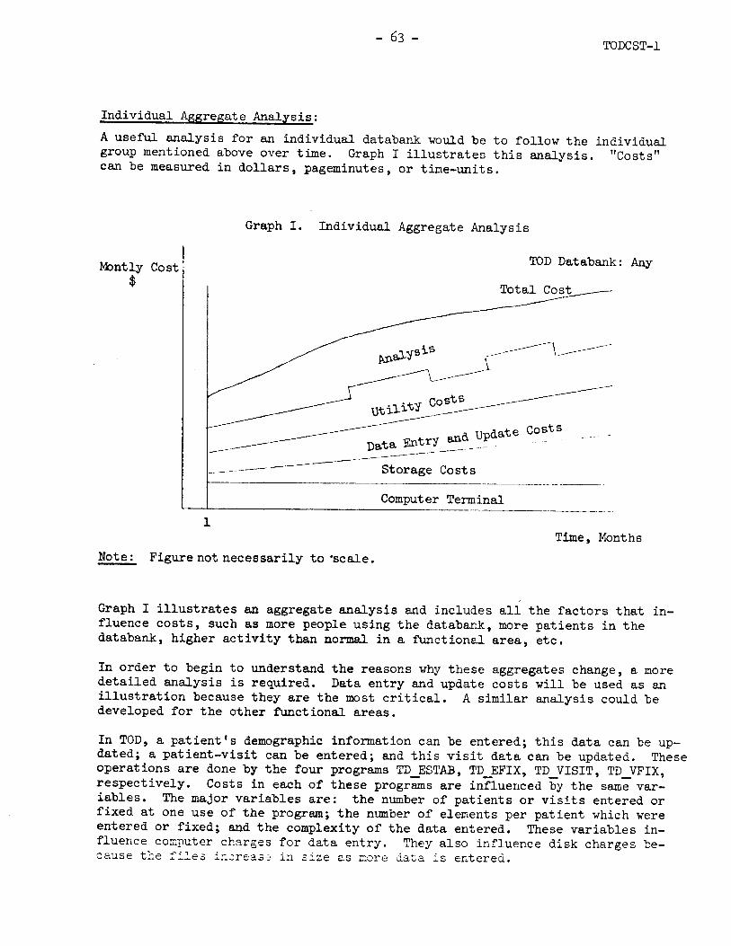
Individual Aggregate Analysis: A useful analysis for an individual databank would be to follow the individual group mentioned above over time. Graph I illustrates this analysis. "Costs" can be measured in dollars, pageminutes, or time-units.

Montly Cost $

Graph I. Individual Aggregate Analysis

TOD Databank: Any

--3 Update Costs --_-- _ Data Entry tuLL

___---- .H

_._ __.. --- ______- /-

Storage Costs

t-

-__-___

Computer Terminal - -- ._-

1 Time, Months

Note: Figurenotnecessarily to 'scale.

Graph I illustrates an aggregate analysis and includes ali the factors that in- fluence costs, such as more people using the databank, more patients in the databank, higher activity than normal in a functional area, etc.

In order to begin to understand the reasons why these aggregates change, a more detailed analysis is required. Data entry and update costs will be used as an illustration because they are the most critical. A similar analysis could be developed for the other functional areas,

In TOD, a patient's demographic information can be entered; this data can be up- dated; a patient-visit can be entered; and this visit data can be updated. These operations are done by the four programs TD_ESTAB, TD_EFIX, TD-VISIT, TDJFIX, respectively. iables.

Costs in each of these programs are influenced by the same var- The major variables are: the number of patients or visits entered or

fixed at one use of the program; the number of elements per patient which were entered or fixed; and the complexity of the data entered. These variables in- fluence computer charges for data entry. They also influence disk charges be- cause the file5 insreaa2 ' in size es mre iaLa is entered.

- 64 - TODCST-1

In looking at the costs of using these programs, the example of entering a patient's demographic information using program TD_ESTAB will be studied. Similar statements can be made for the other programs. (time,

In TD ESTAB, the cost dollars, or pageminutes) per natient entered is useful-because it re-

moves the direct effect of the number of patients entered to yield a more basic cost coefficient. For the same reason, the cost per patient element entered is taken as the elementary cost unit. One could argue that the com- plexity of the element measured in Be-- J-strokes to enter would be the true basic cost unit. At present we are only analyzing down to the element level.

Watching the cost per patient and the cost per element provides useful insight into the data entry costs. If the number of elements added per patient was always about the same, then we wouldn't have to use the cost per element; the cost per patient would do, In Oncology and Immunology, the number of elements entered per patient does vary widely, TD CSTCK does not presently include compile time,

One must remember that the cost of compiling a program is finite and could shadow the effect of entering data. The effects are relative in the sense that 20 elements for a patient might be comparable to one quarter of compile time. In this case, ignoring compile time, which is not accounted for by TD-CSTCK, introduces a sizable error, If 200 elements were entered, the error of not counting compile time becomes negligible.

Having picked cost per element as the elementary item, Graph II illustrates a method of studying it over time. Cost will be measured in minutes per patient element.

Graph II. Elementary Cost Components Vs. Time

TOD Databank: Any Cost, Minutes (

per patient element arting

-si\

out

Newdata entry

-

I ---__-

Time, Months

- 65 - TODCST-1

One would expect variability in this elementary item for several reasons. A badly written TOMP chart with items improperly marked will slow down the data entry operation. Interruptions of the data entry person such as phone calls, visitors, etc., will increase the data entry cost. A new data entry person will take more time until he or she has learned the system. Assuming a con- sistent chart, no interruptions, and the same data entry person, the costs still will vary (e.g. data entry person can become bored or fatigued).

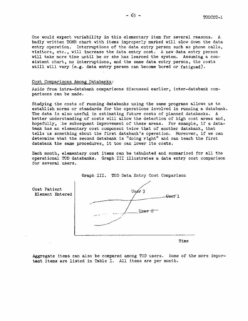
Cost Comparisons Among Databanks: Aside from intra-databank comparisons discussed earlier, inter-databank com- parisons can be made.

Studying the costs of running databanks using the same programs allows us to establish norms or standards for the operations involved in running a databank. The data is also useful in estimating future costs of planned databanks. A better understanding of costs will allow the detection of high cost areas and, hopefully, ;he subsequent improvement of these areas. For example, if a data- bank has an elementary cost component twice that of another databank, that tells us something about the first databank's operation. Moreover, if we can determine what the second databank is "doing right" and can teach the first databank the same procedures, it too can lower its costs.

Each month, elementary cost items can be tabulated and summarized for all the operational TGD databanks. Graph III illustrates a data entry cost comparison for several users.

Graph III. MD Data Entry Cost Comparison

Cost Patient Element Entered

Time

Aggregate items can also be compared among TOD users. Some of the more impor- tant items are listed in Table I. All items are per month.

- 66 - MDCST-1

Table I. TOD Costs Comparison for all TOD Users

Month of: xxxxxxx

ITEM USER 1 USER 2 USER 3 . . .

From ACME Accounting: Terminal Cost. Computer Cost. Number of Pageminutes. Number of Minutes. Number of Blocks.

From TD-CSTCK: Minutes. $ Estimated. Pageminutes Estimated. Cost per Program. Cost per Functional area.

Miscellaneous: Ratio($ fromACMEto $ fromTD CSTCK), Ratio(Time fromACMEtotime fromTD CSTCK). Ratio(Pageminutes fromACMEto pageTfromTD CSTCK). % of cost falling in each functional area: Number of patients in file. Number of patients entered, Number of patient-visits in file. Number of patient-visits entered.

- 67 -

TODCST-1

A final analysis which would illustrate the use of TOD is shown in Graph IV.

Total TOD Computer Charges

Graph IV. Total TOD Computer Charges

General S&!!!Lm

I &gllS

I I I I I I

iseases Clinic

March 1973 Time, Months

Dist: Staff/TOD/All

- 68 =.

Core Research & Development (Continued)

C. New Analysis Programs for Time Series Data Project: ACME Realtime

Investigator: Will Gersch

Dept. of Neurology

1. Description

ARSPEC is an interactive research tool for automatic spectral density analysis of time series data. The program performs four interrelated tasks: (1) display of time series data; (3) data reduction;

(2) filter design and application to data; and (4) spectral density computation. The user instructs

ARSPEC to perform tasks in a desired order by issuing supervisory commands.

Unlike PUBLIC program TIMESER, ARSPEC uses an automatic decision proce- dure to produce accurate spectral estimates. This technique is applicable to all time series data.

The computational procedures are defined in ACME Note EARSPE-2.

2. Historical Note

The recursive procedure for computing autoregressive coefficients is due to Levinson (A)(l$iT). This procedure was "re-discovered" by Durbin

(B) (1960) l The automatic decision procedure for deciding the order of the autoregressive model is due to Akaike (C,E)(1970). An alternate statistical procedure based on earlier statistical procedures for deciding autoregressive model order appears in Gersch (D)(1970).

3. A Short Explanation of Spectral Analysis by Autoregressive I&de1 Technique

Conventional spectral analysis procedures compute spectral density estimates using a weighted Fourier transform of the empirical autocorrelation function of observed time series. The use of conventional techniques is complicated by the requirement that a user assign the values of parameters determining statistical tradeoffs in the spectral representation. This requires expertise with spectral estimation theory. As a case in point, conventional spectral analysis techniques are employed by ACME PUBLIC pro- gram TIMESER.

The autoregressive model technique fits a model to be observed data. This model is autoregressive in that each observation of the time series is expressed as a linear combination of its own past (hence it is regressive on itself) plus a term drawn from an uncorrelated sequence (Equation 1). The coefficients of the model are determined by a least squares fit to the empirical autocorrelation function. The order of the model is determined by the Akaike (E) final predictor error criterion.

- 6g -

Core Research & Development (Continued)

Spectral density estimates are calculated from the coefficients of the autoregressive model (Equation 2).

The statistical performance of spectral estimation using the autore- gressive technique has the properties that (i) the spectral estimates are unbiased, and (ii) the variance of the spectral estimates is approximately given by

vai4f) = N s 't 22 h2(f)

where p = the order of the autoregressive model. The statistical perfor- mance of this procedure is at least as good as the performance of the best conventional spectral estimate. Finally, the fact that the procedure is unbiased eliminates the need for expert determination of the statistical trade-offs, and hence the procedure can be made automatic.

4. References

A. Levinson, N. (1947). The Wiener RMS (Root Mean Square) Error Criterion in Filter Design and Prediction. 5. Math. Physics, z, pp. 261-278.

B. Durbin, J. (1960). The fitting of time-series models. Rev. Int. Stat. Inst. 28, pp. 233-244.

C. Akaike, H., Information theory and an extension of the maximum likelihood principle, presented at the Second International Symposium on Information Theory, Tsahkadsor, Armenian SSR, 2-8 of September, 1971. (To be published in Problems of Control and Information Theory, USSR 1972.)

D. Gersch, W. (1970), "Spectral Analysis of EEG's by Autoregressive Decomposition of Time Series", Mathematical Biosciences, 7, 1970, pp. 205-222.

E. Akaike, H., Statistical Predictor Identification, Ann. Inst. Stat. Math., 21, 1970*

5. Sample Runs

Raw data is a sine wave imbedded in noise. Noise is Gaussian noise with mean zero and standard deviation an order of magnitude greater than the sine wave amplitude. Noise has been passed through a high pass filter before addition to the sine wave.

- 70 -

Core Research & Development (Continued)

Data set number of graphics device=?13 UJ YOU ARE NOW PERMITTED 01 LINES ON TVE 1800 Number of raw data samples=?1000 Name of raw data file =?TEST Key of record containing raw data=?1 Enter a command =?display Enter 0 to operate on raw data, nonzero to operate on orocessed data=?0

DFILE= TEST, DREC= 1

FIGURS 1

- 71 -

Enter ,a co;:li,ian4 =?spectrurn tll tcr r) to operate on t-a\: data, nonzero to operate on processed 4atJ=?Q

= ’ s’.u tor e,;rcss i ve ~horje 1 i s of or.ier ’ , = $3; IJptir~rizl liescri ytion of spectrum =?sine wave in filtered noise ?nter 0 if done, nonzero to save spectrum on data file.=?0

0 SINE Wt3VE IN FIiTERED NOISE

NORriRLIZED FREQUENCY

Figure 2

Enter a command =?fi lter High frequency cutoff point=?O.l Low frequency cutoff=?O.OS Enter 0 for low nass, nonzero for hfy;h pass fi 1 ter=?O Enter 0 for unsmoothed, nontero for smooth4 f f 1 ter=?l Enter 0 to display, nonzero to apply f 11 ter=?O Enter 0 to ooerate on raw data,

I

nonzero to operate on processed data=?0 FILTER DESIGN

1 i

p .0 0.1 0.2 0.3 0.4 0.5

NORMALIZE0 FREQ. I

FIGURE 3

- ‘j-2 -

After filtering, we can see the original sine wave. Enter a cormand =?disp]ay Enter 0 to oneratc on raw data, nonzero to operate on processed dFtaJ?l

PROCESSED DATA

I

FIGURE4

Note the end effects caused by filtering 2 1. The second example is a spectral analysis of actual EEG data,

l’;ta set number of graphics device=?91 liuir!her of t-a{+ .lata sa17ples=?L003 ‘!ar?e of t-a\/ .la ta f i le =?EEGDATA Key of record containing raw data=?100 Enter a command =?display ct-l+er fl tn nnerat0 r>n t-a\: data, norlZer0 to ooerzte nn Drnrcr<pJ ,daf-a=?f

OFILE= EEGORTA, DREC= 100

Figure5

- 73 -

Enter a command =?spectrum Enter !I to operate on raw data, nonzero to operate on processed data=?0

=‘Autoregressive model is of order’,- 22; Optional description of spectrum -?EEG SPECTRUM Enter 0 if done, nonzero to save spectrum on data fIle.=?O

EEG SPECTRUM

I 0.5

NORMRLIZED FREQUENCY

Figure 6

A low pass filter is now applied; then data is reduced to 1000 points.

Enter a command =?fi 1 ter tllgh frequency cutoff point=?0.25 Low frequency cutoff-?0.2 Enter 0 for low pass, nonzero for high pass fl lter=?O Enter 0 for unsmoothed, nonzero for smoothed f i 1 ter=?l Enter 0 to !Jisplay, nonzero to apply fi 1 ter=?l Enter 0 to operate on raw data, nonzero to operate on processed data=?0 Enter a command =?reduce Enter 0 to operi;te on raw data, nonzero to operate on prr>cessefl data=?1 Number of rc(juced data sampl es=?1000 Cnter a command =?spectrum Enter 0 to operate on rat:4 data, nonzero to operate on processed data=?1

-‘Autoregressive model is of order’,= 21; Optional description of spectrum =? Enter 0 if done, nontero to sava spectrum on data file.=?0 Enter a command =?done 0 127: RUN STOPPED

AT LINE 3.100 IN PROCEDURE ARSPEC

- 74 -

!xl I 1 r I 20 - 0.1 kl.2 0.3 0.4 0.5

NORMRLIZEO FREQUENCY

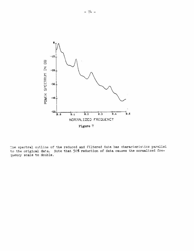
Figure 7

The spectral outline of the reduced and filtered data has characteristics parallel to the original data. Note that 50s reduction of data causes the normalized fre- quency scale to double.

f-- -3 "charh-30

i

- 75 -

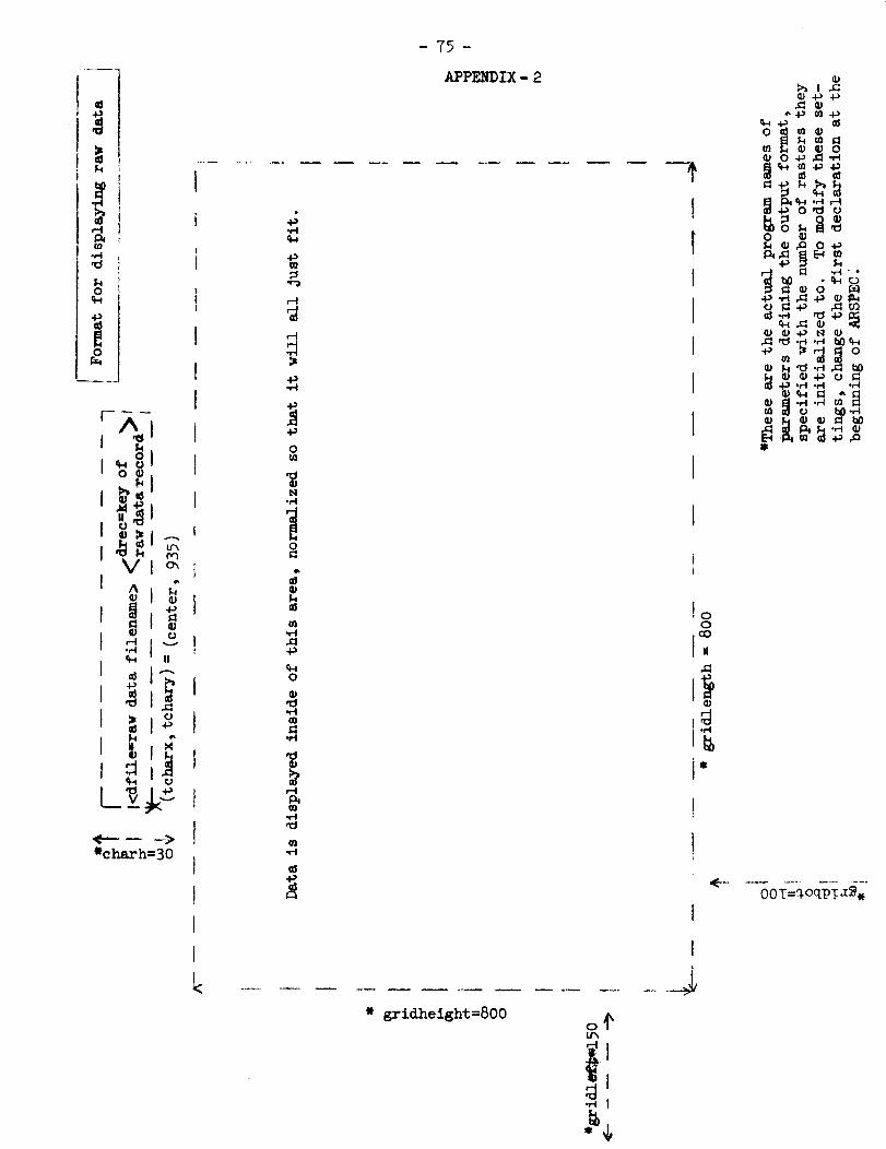
APPENDIX-2

-- _I -- - c_ --- - - - --.

* gridheight= o? 2 1 I

4' .l-i !